Data Analytics for Corrosion Assessment

Abstract

Accurate corrosion detection and prediction requires novel tools for processing surfaces/panels exposed to corrosive environments in order to detect early corrosion initiation. Data analytics offers a rich array of methods execute a sequence of tasks starting with pre-processing of raw images to improve the image to noise ratio, extracting features or useful information from pre-processed images, selecting the “best” features that are characteristic of corrosion evidence, and classifying the features for further processing. We take advantage of classical techniques for data mining but we introduce also new tools based on Deep Learning.

5.1 Introduction

It has been established that corrosion is one of the most important factors causing deterioration, loss of metal, and ultimately decrease of system performance and reliability in critical aerospace, industrial, manufacturing and transportation systems. Corrosion monitoring, data mining, accurate detection and quantification are recognized as key enabling technologies to reduce the impact of corrosion on the integrity of these assets. Accurate and reliable detection of corrosion initiation and propagation with specified false alarm rates requires novel tools and methods. Corrosion states take various forms starting with microstructure corrosion and ending with stress-induced cracking [1–3] (Fig. 5.1).

Fig. 5.1

Microstructure corrosion

Generally speaking, corrosion starts in the form of pitting, owing to some surface chemical or physical heterogeneity, and then facilitated by the interaction of the corrosive environment fatigue cracks initiate from corrosion pitted areas and further grow into the scale that would lead to accelerated structure failure [4]. In order to effectively conduct structural corrosion health assessment, it is thus crucial to understand how corrosion initiates from the microstructure to the component level and how structure corrosion behaviors change as a result of varied environmental stress factors. Many research efforts have been reported in the past addressing this critical issue [5–8]. Traditionally, conventional ultrasonic and eddy current techniques have been used to precisely measure the thickness reduction in aircraft and other structures; there has been a number of undergoing research efforts using guided wave tomography techniques to screen large areas of complex structures for corrosion detection, localization [9] and defect depth mapping [10]. However, due to the nature of ultrasonic guided waves, this technique is vulnerable to environmental changes, especially to temperature variation and surface wetness occurrence [11], and the precision of corrosion defect depth reconstruction is restricted by sensor network layout, structure complexity, among others, which limits the scope of the field application. Thus, undeniably, well-recognized global corrosion measurements, such as material weight loss and wall thickness reduction, cannot offer an appropriate and trustworthy way to interpret the pitting corrosion due to its localized attack nature.

Figure 5.2 is a pictorial representation of the corrosion assessment technologies from corrosion monitoring to data mining, detection/prediction and assessment.

Fig. 5.2

Basic modules of the smart sensing modality

Besides, advanced corrosion health assessment systems require comprehensive quantitative information, which can be categorized into a variety of feature groups, such as corrosion morphology, texture, location, among others. It calls for the exploration of both new testing and data fusion methods from multiple testing techniques. Forsyth and Komorowski [12] discussed how data fusion could combine the information from multiple NDE techniques into an integrated form for structural modeling. Several other studies have looked into different sensing technologies for corrosion health monitoring, including using a micro-linear polarization resistance, μLPR sensor [13, 14], and fiber optic sensors [15]. However, the existing research effort in combination with surface metrology and image processing is very limited. In parallel to the current corrosion sensing technology, there have been a number of corrosion modeling studies trying to numerically capture the processes of pitting corrosion initiation, pitting evolvement, pitting to cracking transition, and crack growth to fracture at the molecular level. However, currently there is no accepted quantitative model to take into consideration the effect of stress factors (e.g., salinity, temperature, humidity, pressure), although the effects of the above-mentioned stress factors have been widely discussed.

We address in this chapter analytical tools and methods to extract useful information from corroding surfaces that will be exploited eventually to assess the health state of critical aircraft, ships, and transportation systems, among others [16]. The architecture is set as a decision support system providing advisories to the operator/maintainer as to the health status of such assets subjected to corrosion and in need of corrective action.

5.2 Corrosion Data Mining-Feature Extraction and Selection

An important and essential component of the corrosion detection and interpretation architecture involves image/characterization data pre-processing and data mining aimed to extract useful and relevant information from raw data. Figure 5.3 depicts the architectural components of the pre-processing, feature extraction, selection and classification steps. The latter is detailed in the sequel.

Fig. 5.3

Corrosion data pre-processing, feature extraction/selection and classification

Features are the foundation for the degradation/corrosion detection and interpretation scheme. Feature extraction and selection processes are optimized to extract only the information that is maximally correlated with the actual corrosion state. Appropriate performance metrics, such as correlation coefficients, Fisher’s Discriminant Ratio (FDR), etc. are utilized to assist in the selection and validation processes. Figure 5.4 shows the overall data mining scheme. Image pre-processing, feature extraction and selection are highlighted leading to their utility in pitting corrosion detection, localization, quantification, and eventually prediction of corrosion states.

Fig. 5.4

Corrosion data mining scheme

5.3 Image Pre-processing

Image/data pre-processing involves filtering and preparing the data for further processing. Figure 5.5 shows a typical sequence of pre-processing steps for corrosion images from surface metrology testing. In the first step, de-noising, discrete stationary wavelet transform (SWT) is applied, and then histogram equalization is performed for contrast enhancement followed by applying a threshold to identify the regions of interest in the image. In this framework, image processing techniques are utilized to pre-process the global test panel images as well as the local pitting area images, in preparation for the feature extraction step. First, globally, for each test panel used to demonstrate the algorithmic developments, successive 2D microscopic images were taken and stitched together to obtain the entire panel image. In the whole panel image pre-processing, the rivet-hole areas and artifacts (e.g., stencil-stamp marked numbers) were manually whitened so they would not be confused with corroded regions. In order to identify the pitting corrosion attacked areas, a 2D median filter was applied followed by thresholding (with a threshold of 0.2) to obtain at a binary image. Second, locally, each suspected pitting area is identified from the whole panel image, and a closer microscopy examination was conducted. An example of a local pit identification process is shown in Fig. 5.6. To identify the pit(s) from the background, the area of each object (i.e., black region representing corroded region) in the binary image was calculated. The sum of objects with the area larger than 50 pixels was defined as the total area of the pitting corroded regions. Note that the identification threshold of 50 pixels was set to avoid mistaking dark regions caused by the grain boundaries as pits.

Fig. 5.5

Corrosion image pre-processing

Fig. 5.6

Local pit identification via image processing. Left: Original localized pit image; Right: Pit identified from the background with the pit edge (in blue) identified by image processing algorithm

5.4 Data Mining/Image Processing

An important and essential component of the corrosion detection architecture involves data/image pre-processing and data mining aimed to extract useful and relevant information from raw data. In the proposed architecture, the most important components supporting the implementation of the algorithm are feature extraction and diagnosis/prognosis models. Features are the foundation for “good” fault/corrosion detection algorithms. Feature extraction and selection processes are optimized to extract only information that is maximally correlated with the actual corrosion state. Appropriate performance metrics are defined to assist in the selection and validation processes. Image/data preprocessing involves filtering and preparing the data for further processing. Figure 5.7 shows a typical sequence of preprocessing steps for corrosion images.

Fig. 5.7

Image preprocessing

Of particular interest to our theme is localized pitting and cracking, i.e. cracking initiating at points on the surface of a specimen (joints, fasteners, bolts, etc.). A metal surface (aluminum alloy, etc.) exposed to a corrosive environment may, under certain conditions experience attack at a number of isolated sites. If the total area of these sites is much smaller than the surface area then the part is said to be experiencing localized corrosion in Fig. 5.8. We exploit novel image processing tools/methods, in combination with other means (mass loss calculations) to identify features of interest to be used in the modeling task, since imaging of corroding surfaces offers a viable, robust and accurate means to assess the extent of localized corrosion (Fig. 5.6).

Fig. 5.8

Left: LEXT OLS4000 3D Laser Measuring Microscope. Right: Bruker’s Dektak^® Stylus Profiler

We use novel microscopy and profilometry image processing equipment in order to obtain images of corroded surfaces and extract from such images relevant information that assists in corrosion modeling, diagnostics and prognostics. In our testing, we are using a laser microscope and a stylus-based profilometer, as shown in Fig. 5.9.

Fig. 5.9

a Whole plate imaging of AA 7075-T6 panel (150.63 × 73.87 mm, 108×). b Area the profilometer covers for the 3D map scan

The LEXT OLS4000 3D Laser Measuring Microscope is designed for nanometer level imaging, 3D surface characterization and roughness measurement. Magnification ranges from 108× to 17,280×. Typical 2D and 3D images are shown in Figs. 5.9a and 5.10, respectively.

Fig. 5.10

Pitted panel area (1278 × 2561 µm, 216×) 3D imaging and corresponding profile info (in µm) on uncoated AA 7075-T6 panel

The Bruker’s Dektak^® Stylus Profiler is a traditional 2D contact profilometer. However, with the programmable map scan capability and the post-processing software, it allows for large area 3D topography coverage. The combination of the two imaging tools facilitates both the localized and global characterization of a corroded panel at various resolution scales. In summary:

• 1. Global characterization:

  • The laser microscope can provide large area 2D microscopy imaging as shown in Fig. 5.9a.

  • The stylus profilometer can provide large area 3D map scan imaging. A schematic of the area the profilometer covers for the 3D map scan for a typical panel is shown in Fig. 5.9b.

• 2. Local characterization:

  • After the detection and localization, the laser microscope can provide a close look at the 3D topography of the analyzed surface. An example of pit profile measurement is shown in Fig. 5.6.

5.5 Feature Extraction and Selection

The images obtained through conventional NDI methods are not directly suitable for identification and quantification of damaged regions. Such images therefore need to be enhanced and segmented appropriately for further image analysis. Segmentation has been achieved using de-noising, contrast enhancement, and threshold techniques. Transform based features such as wavelet coefficients also can be used to quantify the extent of corrosion in the image. Neural networks were applied in the process of segmentation and quantification of damaged regions. Segmentation results show a good correspondence between the extracted regions and the actual damage on sample panels.

Several features may be extracted from corrosion images such as statistical features, transform based features (wavelet), texture features and morphological features. These features are outlined in Tables 5.1, 5.2, 5.3 and 5.4.

Table 5.1 Statistical features

Table 5.2 Wavelet features

Table 5.3 Texture features from gray level co-occurrence matrix (GLCM)

Table 5.4 Morphological features

Figure 5.11 shows a set of example corrosion images that were taken with the LEXT OLS laser measuring microscope. The images were taken of an AA 7075-T6 panel that has an exposure time of 286 h in a cyclic corrosion chamber running the ASTM G85-A5 test. In order to distinguish between images of different levels of corrosion a number of features can be extracted from the images. These features fall under the main categories of statistical features, transform based features (wavelet), texture features and morphological features. The statistical features are summarized in Table 5.1. The mean pixel value, standard deviation and entropy of the example corrosion images in Fig. 5.11 are plotted in Fig. 5.12.

Fig. 5.11

Example corrosion images. Top row: low corrosion. Bottom row: high corrosion

Fig. 5.12

Statistical features of example images shown in Fig. 5.1

Wavelet based features are widely used in the literature for Image processing/data mining applications. The wavelet domain takes advantage of the wavelet capability to resolve images in the spatial and frequency domains. The 2D wavet decomposition pursues the following steps:

• A wavelet transform of a 2D image, I, can be performed by applying a set of band and low pass filters H and L along the rows (x) and columns (y) of the image. The sub-images of the 2D wavelet transform are given by the following equations:

$$ \begin{aligned} A & = \left[ {L_{x} *\left[ {L_{y} *I} \right]} \right]\left( {x,y} \right) \\ D_{H} & = \left[ {L_{x} *\left[ {H_{y} *I} \right]} \right]\left( {x,y} \right) \\ D_{V} & = \left[ {H_{x} *\left[ {L_{y} *I} \right]} \right]\left( {x,y} \right) \\ D_{D} & = \left[ {H_{x} *\left[ {H_{y} *I} \right]} \right]\left( {x,y} \right) \\ \end{aligned} $$

where * denotes convolution, A is the approximation image, D_H is the horizontal detail, D_V is the vertical detail, and D_D is the diagonal detail

• After the band and low pass filters are applied the 4 resulting sub-images are down sampled.

• The sub-images at the next level of thwavelet transform are computed using the same operations on the approximation sub-image from the previous level.

Figure 5.13 shows an example of a 2-level wavelet decomposition of a corrosion image using a Daubechies wavelet (db3). Table 5.2 shows the wavelet features that are extracted at each wavelet decomposition level as outlined by Livens. At each level, k, a total energy feature, $E_{total}^{k}$, was calculated using the horizontal, vertical and diagonal sub-images at level k ($D_{H}^{k} ,D_{V}^{k}$, and $D_{D}^{k}$ respectively). Additionally the anisotropy of the energy (how much the energy differs with direction) was calculated. Figure 5.14 shows the wavelet energy features of the example corrosion images shown in Fig. 5.11. From the graph it is evident that the low corrosion images seem to have higher energy feature values at each level than the high corrosion images.

Fig. 5.13

2 level 2D wavelet decomposition

Fig. 5.14

Wavelet features of example corrosion images shown in Fig. 5.1

Wavelet Feature Extraction and Classification example:

• Step 1: For each 512 × 512 block perform 2D wavelet decomposition as shown in Fig. 5.13. 512 × 512 blocks were taken from images shown in Fig. 5.15. Figure 5.16 shows the processing steps.

  Fig. 5.15

  

  Corrosion image processing

  Fig. 5.16

  

  Images from submersion test used to test wavelet feature extraction method. a Corresponds to “baseline” and b corresponds to “pitted”

• Step 2: Extract energy and Orian features from wavelet coefficients: $E_{total}^{1} ,E_{total}^{2} ,Orian^{1} ,Orian^{2} ,E_{A}$ (see Table 5.2).

• Step 3: Train Learning Vector Quantization (LVQ) Neural Network (shown in Fig. 5.17) with 30 random samples.

  Fig. 5.17

  

  Learning Vector Quantization (LVQ) neural network

• Step 4: Test LVQ with entire set of samples (results shown in Fig. 5.18). Only three pitted images were misclassified as a baseline image (Fig. 5.19).

  Fig. 5.18

  

  Confusion matrix. Class 1 corresponds to pitted images and Class 2 corresponds to baseline image. The Target class is the actual class of the image output class is the predicted class of the image from the LVQ neural network

  Fig. 5.19

  

  GLCM calculation from image

Texture features such as contrast, correlation, energy and homogeneity can be calculated using the gray level co-occurrence matrix (GLCM) of an image (see Table 5.3). The (i, j) value of the GLCM of an image I has the value of how often a pixel value i occurs horizontally adjacent to a pixel with value j in the image I. Figure 5.19 shows a depiction of how to calculate the GLCM matrix from an image I. Example values of the GLCM features calculated using the low and high corrosion images (as shown in Fig. 5.11) are shown in Fig. 5.20. Note that the high corrosion images tend to have higher homogeneity, correlation and energy. This could be due to the large black areas that characterize the high corrosion images.

Fig. 5.20

Contrast, correlation, energy and homogeneity features of low and high corrosion images (Fig. 5.14)

Table 5.4 displays a number of morphological features that can be extracted from a segmented image. Morphological features give information on the type of shapes in the images. Pits tend to be round objects while cracks are longer and tend to have an eccentricity close to 1. An example of Fig. 5.21 shows an example of the roundness feature calculated for an image of pits. These morphological features can be used to characterize the types of different corrosion states in one image (for example identifying a crack or pit in an image) (Fig. 5.22).

Fig. 5.21

Image on the right shows all the objects identified in the image ‘Pit3’ with the roundness metric in pink near the object

Fig. 5.22

Top: Original image with rivets and number removed. Bottom: Binary image after filtering. Black corresponds to corroded regions

The area feature is used to calculate the percentage of corrosion on an entire panel. Figure 5.22 shows a panel from the March 12 2014 lap joint chamber test. The top image is the uncoated 7075-T6 aluminum panel that had an exposure time of 286 h. The bottom image is the binary image of the top image after applying a median filter. From the binary image the percent area of corrosion on the panel can be calculated.

Figure 5.23 shows the progression of corrosion during the March 12 2014 lap joint chamber test through the three images on the left and the graph of their corresponding percent area of corrosion on the right. One of the main disadvantages of using morphological features is that they are very sensitive to the segmentation algorithm that is used (Fig. 5.24).

Fig. 5.23

Percent area of corrosion calculated for 7075-T6 aluminum panels with different exposure times

Fig. 5.24

Surface roughness features

In addition to features that can be extracted from the 2D corrosion images the LEXT OLS4000 3D Laser Measuring Microscope and Veeco Dektak 150 surface profilometer can measure a number of surface roughness and volume features. The surface roughness features are listed in Table 5.5. Note that Z(x, y) is the height of the panel measured over an area, A, of about 39.32 mm × 114 mm using the Veeco Dektak 150 surface profilometer.

Table 5.5 Surface roughness features

Parameters related to the volume of the void portion and the material portion are defined as shown in the diagram in Fig. 5.25. 10 and 80% are default values of the heights for the boundaries among the valley section, core section, and peak section.

Fig. 5.25

Material ratio curve

• V_vv: The void volume of the valley section, as calculated from the material ratio curve

• V_vc: The void volume of the core section, as calculated from the material ratio curve

• V_mp: The material volume of the peak section, as calculated from the material ratio curve

• V_mc: The material volume of the core section, as calculated from the material ratio curve.

Surface roughness and volume features measured using the LEXT OLS4000 3D Laser Measuring Microscope are shown in Figs. 5.28, 5.29 and 5.30. The features were measured from the following panels:

• 1. Baseline sample of AA 2024-T3: Surface profiles are measured including the 2D and 3D profile images and basic profile information, and surface roughness is calculated. Panel shown in Fig. 5.26.

  Fig. 5.26

  

  Two 1.0” × 1.0” AA 2024-T3 and AA 7074-T6 panels prepared for microscopic analysis

• 2. Corrosion Panel #1 of AA 2024-T3 from 2013 – jan 16 BAA-RIF lapjoint cct−10 test: 10 measurement areas of 642 × 644 µm² were randomly selected (close/away from rivet holes) from both coated and uncoated sides for profile the measurement, and 3D surface roughness is calculated for each measurement. This panel is shown in Fig. 5.27; (Table 5.6).

  Fig. 5.27

  

  Corrosion panel #1 of AA2024-T3. a Uncoated side and b coated side

  Table 5.6 Summary of surface profile measurement of Panel #1, AA2024-T3 (“×” represents the measurement is close to a random rivet hole, while the blank represents being away to any rivet holes)

5.6 Baseline Profile Measuring Results

5.6.1 2D Profile Information

• Corrosion Panel #1 Profile Measuring Results (Figs. 5.28 and 5.29)

  Fig. 5.28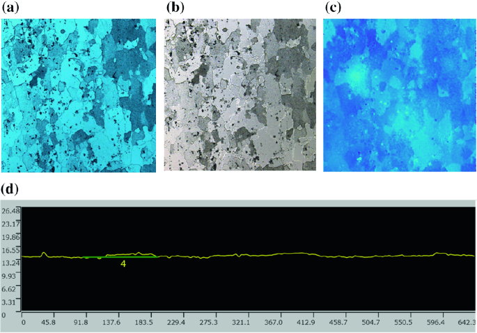

  

  Surface 2D measurement of the AA 2024-T3 baseline sample. a Laser intensity image. b Color image. c Height intensity image. d A cross-section profile

  Fig. 5.29

  

  Surface 2D measurement from panel #1 uncoated side, close to a rivet hole, AA 2024-T3. a Laser intensity image. b Color image. c Height intensity image

5.6.2 2D Profile Information

Pit Profile Information:

In Fig. 5.30, the cross-sectional (CS) area of the highlighted pit profile is 240.43 µm².

Fig. 5.30

A pit profile from Panel #1, uncoated side, away from rivet holes, AA 2024-T3

In Table 5.7, the average pit width is 96.06 µm and the average pit height is 13.74 µm.

Table 5.7 Typical pit profile information from Panel #1, coated, AA 2024-T3

In Table 5.8, the average CS area is 354.435 µm².

Table 5.8 Typical pit CS areas from Panel #1, uncoated, AA 2024-T3

5.6.3 3D Profile Information

• 1. 3D Images.

• 2. 3D Surface Roughness Measurement.

5.7 Cut-off Wavelength λ_c Selection

During an area surface roughness calculation with a profile measurement gauge, irregularities of the surface profile are filtered by introducing an appropriate limiting filter cut-off wavelength λ_c, as indicated in Fig. 5.36. In order to select λ_c, we need to find out defects of interest to us (e.g. pits) size irregularities by analyzing the surface profiles (Figs. 5.31, 5.32 and 5.33).

Fig. 5.31

3D profile image from Panel #1, uncoated side, AA 2024-T3

Fig. 5.32

Software interface for area surface roughness calculation

Fig. 5.33

Range of surface profile components with standard separation of waviness and roughness according to filtration of irregularities by cut-off wavelengths

The surface irregularities in this application are some manual scratches on the panels as shown below. The defects’ range is over 700 µm, the profile is as shown in Fig. 5.34, and the defect profile information is compared to a typical pit in the same panel side as shown in Fig. 5.35.

Fig. 5.34

Surface defects in the corroded panel 1 of AA 2024-T3

Fig. 5.35

Profile size comparison (No. 1, 3 corresponding to the manual scratch, and No. 2 corresponding to a typical corrosion pit)

After analyzing a number of corrosion pit profiles and comparing with surface defects (e.g. manual scratches), we chose the cutoff wavelength λ_c of 500 µm for the area surface roughness calculation.

From Fig. 5.36 it is obvious that when λ_c of 500 µm is applied, the majority of the interest surface features are captured by the filtered surface roughness image, instead of the waviness image.

Fig. 5.36

2D height intensity images for area surface roughness calculation when λ_c of 500 µm applied. a Surface roughness image. b Waviness image

5.8 Deep Learned Features (DLF)

The widely variable states of corrosion are notoriously difficult to measure and detect, especially at early stages when an insidious problem does not surface until catastrophe strikes. Fast, accurate, automated expert assessment of corrosion can help minimize damage by guiding the condition-based maintenance of structures, as well as the design and use of sensors, from development in the lab to field deployment on aircraft, bridges, etc. A required essential capability in such expert systems is the extraction of features (patterns) from measurements.

Traditionally, feature formulas are hand-engineered by domain experts. For example, in a black-and-white image of pitting formations, a measure of roundness of the contours of pits can be devised. But this assumes that we can automatically delineate the contours of each pit to begin with—useful at later stages of processing but circular logic at the beginning. The issue in this example is that roundness is a feature of the objects of interest (pits), not a feature of a whole image. It is important to be able to examine both local features (e.g., to detect potentially costly small cracks) and global features such as texture-based averages (e.g., if condition is uniform corrosion then situation is relatively benign). An even better approach would be to augment this capability with features that are hierarchically represented (covering a spectrum from local to global) and automatically learned, as happens in natural biological vision systems [LeCun cat’s visual cortex].

Recent breakthroughs in machine learning have enabled unsupervised (i.e., from input data only, without notion of desired outputs) feature learning and massively larger neural networks to be built from training data than was originally possible (e.g., with billions of parameters), in a branch of AI loosely termed Deep Learning [Hinton 2006, DL papers, …]. Our goal is to develop a Deep-Learned Features (DLF) framework that automatically learns neural features from data, to enhance the engineered local/global feature library for corrosion. Advantages of this approach include: (1) ability to learn from data even if a large fraction is unlabeled (no ground-truth labels/classes of corrosion available); (2) ability to use the whole grayscale or color space without necessarily relying on black-and-white binarization (on which morphological filters work best); (3) scalability to very large problems (e.g., 1000-class recognition, using GPUs if needed); (4) hierarchical representations in which some neurons may respond selectively to particular localized corrosion problems, as well as more global, protodetector types of features to include in our library. A disadvantage is that the method tends to require many examples (order to thousands) before generalizing (i.e., able to also work on unseen data) features can be distilled.

Similar technology is being researched and commercially developed by several companies. For example, forms of deep learning networks were used in Google Brain to automatically learn neurons that respond to cats from YouTube video thumbnails, in Google + Photo Search to detect over 1000 objects of scenes without metadata, in Android speech recognition, in parts of IBM Watson, and in a Microsoft real-time English-to-Mandarin translation demonstration. Facebook, Yahoo, and others have expressed interest at NIPS conferences. Additionally, several image classification public competitions have been won by groups using ensembles of deep networks [refs].

5.9 Methods

Our description is geared towards image data, however, similar principles are applicable to other forms of raw input data, such as time-series measurements obtained from µLPR or other sensors.

A classic solution to classification, regression, or PDF estimation problems using artificial neural networks (NNs) involved the 2- or 3-layer multilayer perceptron architecture, a training dataset of M examples with input vectors x ∈ ℝ^N and desired outputs y ∈ ℝ^P, {(x, y)⁽¹⁾, (x, y)⁽²⁾, …, (x, y)^(M)} (the fact that us teachers present desired outputs is what makes this problem “supervised learning”), trained using backpropagation to simultaneously adjust the weight matrices W_i and bias vectors b_i of each layer so as to minimize mean squared error $E\left\{ {\mathbf{{y}} - {\hat{\mathbf{y}}}^{2} } \right\}$ between inputs and outputs, possibly regularized to encourage generalization over as yet unseen input data. A two-layered network computes the function ${\hat{\mathbf{y}}}\varvec{\sigma}\left( {{\mathbf{W}}_{2}\varvec{\sigma}\left( {{\mathbf{W}}_{1} {\mathbf{x}} + {\mathbf{b}}_{1} } \right) + {\mathbf{b}}_{2} } \right)$, where ⎕(z) = 1/(1 + exp(–z)) is the logistic sigmoid function.

We can think of an input image as a long column vector x containing the pixel intensities (for RGB color, triple the length). Each the K rows of W₁ can be seen as the coefficients of a linear filter with which the dot product between image and filter is computed. The output o ∈ [0,1] of the sigmoid activation function, after passing thru it the dot product plus bias, can be interpreted in our framework as a neural feature. Our DLF framework shares commonalities with the traditional NN setup, but tends to differ in emphasis (harvesting of the neural features inside NN, instead of the NN outputs), supervision levels required for learning (staged between unsupervised and supervised), objective functions being optimized (e.g., addition of sparsity term), use on nontrainable sublayers (e.g., convolution, subsampling, local contrast normalization, etc.), and scalability to more and bigger layers working around the issue of vanishing or exploding gradients that plagued traditional NNs.

Our DLF approach includes the following basic strategies:

• Obtain very large number of possibly unlabeled (i.e., without known/ground-truth output) images, and some labeled images (i.e., with desired output classes y^(m), such as [0 0 1 0]^T indicating the 3rd class in a 4-class problem).

• Preprocess input images to have zero mean, and decorrelated and equally scaled dimensions. This is known as zero-phase component analysis (ZCA) whitening, a type of sphering.

• Unsupervised-learning stage:

  • 1. From unlabeled data, learn neural features via sparse autoencoder (AE) using backpropagation.

  • 2. If necessary, greedily train more AEs in a stack (i.e., pretrain each AE independently of rest of the network, as opposed to all layers jointly).

• Supervised-learning stage: From labeled data, train a classification layer and/or tune whole network using backpropagation.

• Scale up to big images (probably anything above 64 × 64) by randomly sampling small patches (e.g., 16 × 16) and inserting convolution and pooling operations between layers.

We provide more details of these strategies next.

• Prewhitening

• Sparse Autoencoder

Minimize the scalar objective function

$$ J = \frac{1}{2}\left\langle {\left\| {{\mathbf{x}} - {\hat{\mathbf{x}}}} \right\|^{2} } \right\rangle + \frac{\lambda }{2}\sum \left( {w_{ij}^{\left( l \right)} } \right)^{2} + \beta \sum KL(\rho ||\hat{\rho }_{j} ) $$

Stacked Autoencoders

Convolutional Feature Extraction

Supervised Stage

5.10 Codebase Validation

Starting from the stanford_dl_ex MATLAB stubs [Ng refs], we derived all the equations and generated and unit-tested all the code for sparsity-based MSE and cross-entropy cost functions, efficient backpropagation-based gradients, stacked AEs, convolutional and pooling layers, mini-batch stochastic gradient descent, required for the DLF framework. We validated the codebase with several experiments using known real-world big data sets including CIFAR-10, MNIST, and STL-10, achieving expected accuracies from ~81 to 98% when tested over thousands of independent examples unseen during training. We have tens of images of corrosion states which is not yet enough to extract generalizing features. Until thousands of images can be obtained, we also verified the applicability of the method to corrosion using simulated sticks versus circles as proxies for cracks and pits.

• Synthetic Images Verification for Corrosion—the following figures illustrate the procedural steps for corrosion image verification.

5.11 Conclusion

Extending this work to thousands of corrosion images (from confocal microscopy in the lab plus photorealistic simulation), our DLF framework is poised to add powerful, deep-learned feature vectors (e.g., the 9-dimensional pooled features in figure above) to the engineered feature library. Future investigations should examine other hybrid architectures in which, for example, DLF serves as 1st-pass processor to guide the segmentation of regions of interest in corrosion images, a pre-requisite for the engineered local features to work well.

5.12 Feature Selection

Feature selection methods fall under three main categories: wrapper methods, embedded methods, and filter methods.

Wrapper methods assign value to as set of features by the performance of the data mining algorithm. Figure 5.37 shows a schematic of a generic wrapper method. The value of the subset of extracted features in this case is the accuracy of the data mining task using the subset of features from the training set. D. Garrett et al. implemented this approach for a classification task by using a genetic algorithm to search through the extracted feature space and a support vector machine to perform the classification [4]. Other popular search strategies in the literature include: best-first, branch-and-bound, and simulated annealing [5]. In addition, decision trees, naïve Bayes, and least-square linear predictors are popular data mining algorithms used for performance evaluation [5]. Table 5.5 lists various data mining algorithms that can be used to assess the performance of a set of features. One of the main disadvantages of wrapper methods is that they can be computationally intensive.

Fig. 5.37

Schematic of general wrapper feature selection method

In embedded methods the search for the optimal subset of extracted features is built into the classifier construction. Therefore, the search is in the combined space of feature subsets and hypotheses for the classification.

Filter methods assign value to features only by looking at intrinsic properties of the data and are independent of the chosen data mining algorithm. Feature ranking is a filter method for feature selection. Consider a supervised learning problem where there is a set of m observations $\left\{ {f_{1,\;k} , \ldots ,f_{n,\;k} ,y_{k} } \right\}$ (k = 1,…, m). Where $\left\{ {f_{1} , \ldots ,f_{n} } \right\}$ is the set of n extracted features and y is the desired output. The value of f_i is computed using a scoring function which compares f_i to y. For example, for linear regression the squared value of the estimate of the Pearson Correlation Coefficient is used as the scoring function. The estimate of the Pearson Correlation Coefficient is given as:

$$ R\left( i \right) = \frac{{\mathop \sum \nolimits_{k = 1}^{m} \left( {f_{i,\;k} - \overline{f}_{i} } \right)\left( {y_{k} - \overline{y} } \right)}}{{\sqrt {\mathop \sum \nolimits_{k = 1}^{m} \left( {f_{i,\;k} - \overline{f}_{i} } \right)^{2} \mathop \sum \nolimits_{k = 1}^{m} \left( {y_{k} - \overline{y} } \right)^{2} } }} $$

where the bar notation stands for an average over the index k. $R\left( i \right)^{2}$ is used as a scoring function since it represents the fraction of total variance around the mean value $\overline{y}$ that is explained by the linear relation between f_i and y [5]. Table 5.9 lists several data mining methods. Table 5.10 lists advantages, disadvantages and examples as pointed out by Y. Saeys et al. in their review of feature selection techniques.

Table 5.9 Data mining methods

Table 5.10 Advantages, disadvantages and examples of feature selection methods [6]

5.13 Classification Techniques

• Decision Trees [2]

  Let S be a set of cases. Each case consists of a fixed set of attributes (features) and belongs to one of a small number of classes. Given a new case the decision tree will classify the new case based on the known set S.

  Algorithm for Decision Tree:

  • If all the cases in S belong to the same class or S is small, the tree is a leaf labeled with the most frequent class in S.

  • Otherwise, choose a test based on a single attribute with two or more outcomes. Make this test the root of the tree with one branch for each outcome if the test, partition S into corresponding subsets S₁, S₂,… according to the outcome for each case, and apply the same procedure recursively to each subset.

• Ruleset classifiers [2]

  • Consists of a list of rules of the form “if A and B and C … then class X”, where rules for each class are grouped together. A case is classified by finding the first rule whose conditions are satisfied by the case; if no rule is satisfied, the case is assigned to a default class.

  • Rulesets are formed from the initial (unpruned) decision tree. Each path from the root of three to a leaf becomes a prototype rule whose conditions are the outcomes along the path and whose class is the label of the leaf. This rule is then simplified by determining the effect of discarding each condition in turn.

  • A subset of simplified rules is selected for each class in turn.

  • Principal disadvantage is the amount of CPU time and memory required.

• Support vector machines (SVM) [2]

  • In a two-class learning task, the aim of SVM is to find the best classification function to distinguish between members of the two classes in the training data.

  • For a linearly separable dataset, a linear classification function corresponds to a separating hyper-plane f(x) that passes through the middle of the two classes, separating the two.

  • SVM finds the best function that maximizes the margin between the two classes.

  • An SVM classifier attempts to maximize the following function with respect to $\varvec{\overset{\lower0.5em\hbox{$\smash{\scriptscriptstyle\rightharpoonup}$}} {w} }\,{\text{and}}\,b:L_{p} = \frac{1}{2}\left| {\left| {\varvec{\overset{\lower0.5em\hbox{$\smash{\scriptscriptstyle\rightharpoonup}$}} {w} }} \right|} \right| - \varvec{ }\mathop \sum \nolimits_{i = 1}^{t} \alpha_{i} y_{i} \left( {\varvec{\overset{\lower0.5em\hbox{$\smash{\scriptscriptstyle\rightharpoonup}$}} {w} } \bullet \varvec{\overset{\lower0.5em\hbox{$\smash{\scriptscriptstyle\rightharpoonup}$}} {x} }_{i} + b} \right) + \mathop \sum \nolimits_{i = 1}^{t} \alpha_{i}$

where t is the number of training samples, and $\alpha_{i}$, i = 1,…,t are non-negative numbers such that the derivatives of L_p with respect to $\alpha_{i}$ are zero.

Clustering Techniques:

• K-means algorithm [2]

  The algorithm operated on a set of d-dimensional vectors, $D = \{ x_{i} |i = 1, \ldots ,N\}$, where $x_{i} \in {\mathbb{R}}^{d}$ denotes the ith data point.

  • The algorithm is initialized by picking k points in ${\mathbb{R}}^{d}$ as the initial k cluster representatives or “centroids”.

  • The algorithm then iterated between two steps until convergence:

    • Step 1: Data Assignment. Each data point is assigned to its closest centroid, with ties broken arbitrarily. This results in a partitioning of the data.

    • Step 2: Relocation of the “means”. Each cluster representative is relocated to the center (mean) of all the data points assigned to it.

  • Disadvantages of the algorithm:

    • Sensitive to initial centroids

    • Fill falter when the data if not well described by reasonably separated spherical balls

Sensitive to outliers.

5.14 Sensor Data Fusion

Although significant achievements have been reported in the recent past, the processing of sensor data intelligently still requires the development, testing, and validation of new techniques to manage and interpret the increasing volume of data and to combine them as they become available from multiple and diverse sources. Sensor data fusion is a promising technology that can contribute significantly towards a better understanding and a more efficient utility of raw data by reducing it to useful information [17]. We are introducing in this proposal new and innovative fusion techniques that build upon current data management practices but also advance the state of the art through a systems engineering process that is rigorous and verifiable. We define the fusion problem in a generic framework. A methodology is sought using intelligent decision making tools through which data collected from a variety of sensors under various testing, modeling or field conditions can be aggregated in a meaningful and systematic way to provide information to the decision makers at the operational task level. We synthesize the information to higher informational levels. A typical sensor data fusion paradigm incorporates several levels of abstraction: fusion at the data level, the feature (characteristic signature of the fault or failure data) level, the sensor level and the knowledge level. At the data level, a variety of filtering, data compression and data validation algorithms are employed to improve such indicators as signal to noise ratio, among others. The enabling technologies at the feature level borrow from Dempster-Shafer theory, soft computing and Bayesian estimation to fuse feature while meeting specified performance metrics [18]. At the sensor level, we rely upon concepts from information theory while multiple sensors are gated and coordinated spatially and temporally to minimize their number while maximizing the probability of detection. Significant reduction of the computational burden is always a desired objective. The top level of the fusion hierarchy, i.e. the knowledge fusion module is designed to reason about the evidence provided by the lower echelons, aggregate the available information in an intelligent manner, resolve conflicts and report to the end-use the findings of the fusion architecture. Artificial Intelligences (AI) tools and methods from Dempster-Shafer theory, Bayesian estimation techniques and soft computing may find utility as the reasoning enablers at this level.

5.14.1 Fusion at the Feature Level

Feature fusion has attracted the attention of the research community in recent years, as data and data acquisition/processing strategies proliferate, in order to maximize the value of information extracted from raw data while improving the algorithms’ computational efficiency [19–22]. Fused features (meta-features, synthetic features, as sometimes called) improve the performance of diagnostic and prognostic algorithms by increasing the correlation of the constituent features with respect to ground truth fault data. The feature level offers the most advantageous and beneficial opportunity for the application of novel fusion techniques. It is common practice to employ high-bandwidth dynamic sensing modalities (vibration, dynamic pressure, etc.) in order to monitor key attributes of fault/failure modes for critical components/subsystems.

The fundamental principle of fusion algorithms is rather simple: maximize a utility or objective/fitness function that conveys the relationship between the fused features and the actual fault dimension. A number of fusion algorithms, fitness functions and optimization solvers have been proposed over the past years. The challenge stems primarily from the need to define an optimum feature vector and to select the most appropriate fitness function for the problem at hand. The fitness function generally attempts to capture the “similarity” between the fused features and ground truth.

Typical features or CIs in the time domain may include peak values, RMS, energy, kurtosis, etc. in the frequency domain, we focus primarily on features for rotating equipment that exhibit a marked difference between baseline or no-fault and faulty data [23]. For example, we seek in this category a comparison (amplitude, energy, etc.) of certain sidebands to dominant frequencies, when the sensor signals are transformed via an FFT routine to the frequency domain²⁰. Other possible features are extracted through coherence and correlation calculations. When the information is shared between the time and frequency domain, it might be advantageous to extract features in the wavelet domain offering an appropriate tradeoff between the two domains. When multiple features are extracted for a particular fault mode, it is desirable to combine or fuse uncorrelated features to enhance the fault detectability.

Consider the objective or fitness function:

$$ f = \left| {correlation\left( {x,w} \right)} \right| \times FDR\left( {x,w} \right) $$

where x and w could represent two features.

Other suitable fitness functions may be defined depending on the problem at hand. The choice of the “best” fitness function is a challenging task and the most significant step in the optimization process. Once the fitness function and appropriate initial conditions in the search space are given, the algorithm (PSO, GP, etc.) is allowed to run until specified termination conditions are satisfied.

Well established tools like Principal Component Analysis (PCA) and methods based on the degree of overlap between the probability density functions of features are employed first to screen features, prioritize and rank them for further processing. Thus, we face eventually only a subset of the “best” features extracted from raw data.

It is preferable to view features and their corresponding fused versions in a probabilistic or statistical setting. Bayesian estimation methods, Kalman filtering, particle filtering, etc., allow for information from multiple measurement sources to be fused in a principled manner. Typically, multiple snapshots or windowed data are used to extract a feature. A histogram is built next from the feature sequence approximating a Probability Density Function (PDF). Similar constructs are determined from other features from baseline and fault data. Since fusion, regardless of the method employed, is viewed as an optimization problem, an appropriate fitness or objective function must be defined to evaluate each feature. In our brain research work, we defined and employed successfully the following fitness function [24]:

$$ fitness = \frac{{\sqrt {\sigma_{1}^{2} + \sigma_{2}^{2} } }}{{\left| {\mu_{1} - \mu_{2} } \right|}} \times \left( {\frac{1}{{1 - PDF_{overlap} }}} \right) $$

where $\mu_{1} , \mu_{2}$ are the means and $\sigma_{1} , \sigma_{2}$ the standard deviations of two features. The PDF overlap is the common area between the given feature PDF and one obtained from data under no fault conditions. Here, we are attempting to discriminate or distinguish between features belonging to the two classes only: One class representing baseline or no fault conditions and the second representing a faulty stat. Thus, the fitness function is composed of the inverse square root of the Fisher Discriminant Ratio (FDR) divided by one minus the PDF overlap [25].

FDR measures the distance between two classes of features. Sometimes seemingly good FDR values still produce features with large overlaps in the feature histograms for the two classes. This fitness function penalizes features with large class overlaps by increasing the fitness score in proportion to the amount of overlap. The overlap values range from 0 for no overlap to 1 for total overlap. The feature with the lowest fitness score is selected as the best.

5.15 Epilogue

This chapter describes rigorous tools/methods for processing corrosion imaging data. An array of approaches to data mining, feature extraction and selection and classification are presented with extensive examples illustrating the efficacy of these methods. The enabling technologies cover a wide spectrum of innovative legacy and new advances like Deep Learned Features borrowed from the Deep Learning domain. The contents of this chapter set the stage for accurate corrosion detection and prediction algorithms.

References

Hoeppner DW, Chandrasekaran V, Taylor AMH (1999) Review of pitting corrosion fatigue models. In: International committee on aeronautical fatigue, Bellevue, WA, USA
Kawai S, Kasai K (1985) Considerations of allowable stress of corrosion fatigue (focused on the influence of pitting). Fatigue Fract Eng Mater Struct 8(2):115–127
Lindley TC, Mcintyre P, Trant PJ (1982) Fatigue-crack initiation at corrosion pits. Metals Technol 9(1):135–142
Pidaparti RM (2007) Strucural corrosion health assessment using computational intelligence methods. Struct Health Monit 6(3):245–259
Frankel GS (1998) Pitting corrosion of metals: a review of the critical factors. J Electrochem Soc 145(6):2186–2198
Huang T-S, Frankel GS (2006) Influence of grain structure on anisotropic localized corrosion kinetics of AA7xxx-T6 alloys. Corros Eng Sci Technol 41(3):192–199
Szklarska-Smialowska Z (1999) Pitting corrosion of aluminum. Cossorion Sci 41(9):1743–1767
Pereira MC, Silva JW, Acciari HA, Codaro EN, Hein LR (2012) Morphology characterization and kinetics evaluation of pitting corrosion of commercially pure aluminum by digital image analysis. Mater Sci Appl 3(5):287–293
Clark T (2009) Guided wave health monitoring of complex structures. Imperial College London, London
Belanger P, Cawley P, Simonetti F (2010) Guided wave diffraction tomography within the born approximation. IEEE Trans UFFC 57:1405–1418
Li H, Michaels JE, Lee SJ, Michaels TE, Thompson DO, Chimenti DE (2012) Quantification of surface wetting in plate-like structures via guided waves. AIP Conf Proc Amn Inst Phys 1430(1):217
Forsyth DS, Komorwoski JP (2000) The role of data fusion in NDE for aging aircraft. In: SPIE aging aircraft, airports and aerospace hardware IV, vol 3994, p 6
Brown D, Darr D, Morse J, Laskowski B (2012) Real-time corrosion monitoring of aircraft structures with prognostic applications. In: Annual conference of the prognostics and health management society, vol 3
Brown DW, Connolly RJ, Laskowski B, Garvan M, Li H, Agarwala VS, Vachtsevanos G (2014) A novel linear polarization resistance corrosion sensing methodology for aircraft structure. In: Annual conference of the prognostics and health management society, vol 5, no 33
McAdam G, Newman PJ, McKenzie I, Davis C, Hinton BR (2005) Fiber optic sensors for detection of corrosion within aircraft. Struct Health Monit 4:47–56
Sharland SM (1987) A review of the theoretical modeling of crevice and pitting corrosion. Pergamon J Ltd 27(3):289–323
Liggins M, Hall DL, Linas J (2008) Multisensor data fusion: theory and practice. CRC Press, Boca Raton
Dar I, Vachtsevanos G (1997) Feature level sensor fusion for pattern recognition using an active perception approach. In: Proceedings of IS&T/SPIE’s electronic imaging ’97: Science and Technology, San Jose, CA, February 8–14, 1997
Vachtsevanos G, Lewis G, Roemer M, Hess A (2006) Intelligent fault diagnosis and prognosis for engineering systems. Wiley, Hoboken
Wang F, Sun F, Cao B (2007) Feature fusion of mechanical faults based on evolutionary computation. Insight 49(8):471–475
Voulgaris Z, Sconyers C, Vachtsevanos G (2006) A particle swarm optimization approach to feature fusion for failure prognosis of engineering systems. In: Proceedings of 18th mediterranean conference on control and automation, June 2010, Morocco, pp 339–344
Wu B, Saxena A, Partrick R, Vachtsevanos G (2005) Vibration monitoring for fault diagnosis of helicopter planetary gears. In Proceedings of the 16th IFAC
López De La Cruz J, Lindelauf RHA, Koene L, Gutiérrez MA (2007) Stochastic approach to the spatial analysis of pitting corrosion and pit interaction. Electrochem Commun 9(2):325–330
Burrell L, Litt B, Vachtsevanos G (2007) Evaluation of feature selection techniques for analysis of functional MRI. In Proceedings of the 2007 international conference on data mining, Las Vegas, NV, June 25–28, 2007
Burrell L, Glynn S, Vachtsevanos G, Litt B (2007) Feature analysis of functional MRI for discrimination between normal and epileptogenic brain. In: European control conference, Kos, Greece
Author information
Authors and Affiliations
Corresponding author
Editor information
Editors and Affiliations
Rights and permissions
Copyright information
© 2020 Springer Nature Switzerland AG
About this chapter
Cite this chapter
Vachtsevanos, G. (2020). Data Analytics for Corrosion Assessment. In: Vachtsevanos, G., Natarajan, K., Rajamani, R., Sandborn, P. (eds) Corrosion Processes. Structural Integrity, vol 13. Springer, Cham. https://doi.org/10.1007/978-3-030-32831-3_5
Download citation
DOI: https://doi.org/10.1007/978-3-030-32831-3_5
Published:
Publisher Name: Springer, Cham
Print ISBN: 978-3-030-32830-6
Online ISBN: 978-3-030-32831-3
eBook Packages: EngineeringEngineering (R0)