BCARET Model Checking for Malware Detection

Abstract

The number of malware is growing fast recently. Traditional malware detectors based on signature matching and code emulation are easy to bypass. To overcome this problem, model-checking appears as an efficient approach that has been extensively applied for malware detection in recent years. Pushdown systems were proposed as a natural model for programs, as they allow to take into account the program’s stack into the model. CARET and BCARET were proposed as formalisms for malicious behavior specification since they can specify properties that require matchings of calls and returns which is crucial for malware detection. In this paper, we propose to use BCARET for malicious behavior specification. Since BCARET formulas for malicious behaviors are huge, we propose to extend BCARET with variables, quantifiers and predicates over the stack. Our new logic is called SBPCARET. We reduce the malware detection problem to the model checking problem of PDSs against SBPCARET formulas, and we propose an efficient algorithm to model check SBPCARET formulas for PDSs.

1 Introduction

The number of malware is growing fast in recent years. Traditional approaches including signature matching and code emulation are not efficient enough to detect malwares. While attackers can use obfuscation techniques to hide their malware from the signature based malware detectors easily, the code emulation approaches can only track programs in certain execution paths due to the limited execution time. To overcome these limitations, model-checking appears as an efficient approach for malware detection, since model-checking allows to check the behaviors of a program in all its execution traces without executing it.

A lof of works have been investigated to apply model-checking for malware detection [2,3,4, 7, 10,11,12]. [4] proposed to use finite state graphs to model the program and use the temporal logic CTPL to specify malicious behaviours. However, finite graphs are not exact enough to model programs, as they don’t allow to take into account the program’s stack into the model. Indeed, the program’s stack is usually used by malware writers for code obfuscation as explained in [5]. In addition, in binary codes and assembly programs, parameters are passed to functions by pushing them on the stack before the call is made. The values of these parameters are used to determine whether the program is malicious or not [6]. Therefore, being able to record the program’s stack is critical for malware detection. To this aim, [10,11,12,13] proposed to use pushdown systems to model programs, and defined extensions of LTL and CTL (called SLTPL and SCTPL) to precisely and compactly describe malicious behaviors. However, these logics cannot specify properties that require matchings of calls and returns, which is crucial to describe malicious behaviours [8]. Let us consider the typical behaviour of a spyware to illustrate this. The typical behaviour of a spyware is seeking personal information (emails, bank account information,...) on local drives by searching files that match specific conditions. To do that, it has to search directories of the host to look for interesting files whose names match a certain condition. If a file is found, the spyware will invoke a payload to steal the information, then continue looking for the remaining matching files. If a folder is found, it will pass into the folder path and continue investigating the folder recursively. To obtain this behavior, the spyware first calls the API FindFirstFileA to search for the first matching file in a given folder path. After that, it has to check whether the call to the API function FindFirstFileA is successful or not. When the function call fails, the spyware will call the API GetLastError. Otherwise, when the function call succeeds, a search handle h will be returned by FindFirstFileA. There are two possibilities in this case. If the returned result is a folder, it will call the API function FindFirstFileA again to search for matching results in the found folder. If the returned result is a file, it will call the function FindNextFileA using h as first parameter to look for the remaining matching files. This behavior cannot be described by LTL or CTL since it requires to express that the return value of the API function FindFirstFileA should be used as input to the function FindNextFileA.

CARET was introduced to express linear-temporal properties that involve matchings of calls and returns [1] and CARET model-checking for PDSs was considered [6, 7]. However, the above behaviour cannot be described by CARET since it is a branching-time property. To specify that behaviour naturally and intuitively, BCARET was introduced to express these branching-time properties that involve matchings of calls and returns [8]. Using BCARET, the above behavior can be expressed by the following formula:

$$\begin{aligned} \varphi _{sb} = \bigvee _{d \in D} EF^g&\Bigg ( call(FindFirstFileA) \wedge EX^a (eax = d) \wedge AF^a \\&\quad \bigg ( call(GetLastError) \vee call(FindFirstFileA) \\&\qquad \vee \Big ( call(FindNextFileA) \wedge d \varGamma ^* \Big ) \bigg ) \Bigg ) \end{aligned}$$

where the $\bigvee$ is taken over all possible memory addresses d that contain the values of search handles h in the program, $EX^a$ is a BCARET operator saying that “next in some run, in the same procedural context”; $EF^g$ is the standard CTL EF operator (eventually in some run), while $AF^a$ is a BCARET operator stating that “eventually in all runs, in the same procedural context”.

In binary codes and assembly programs, the return value of an API function is placed in the register eax. Therefore, the return value of FindFirstFileA is the value of the register eax at the corresponding return-point of the call. Then, the subformula $(\text {call(FindFirstFileA)} \wedge EX^{a} (eax=d))$ expresses that there is a call to the API function FindFirstFileA whose return value is d (the abstract successor of a call is its corresponding return-point). A call to FindNextFileA requires a search handle h as parameter and h must be put on top of the program’s stack (as parameters are passed through the stack in assembly programs). To express that d is on top of the program stack, we use the regular expression $d \varGamma ^*$. Thus, the subformula $[\text {call(FindNextFileA)} \wedge d \varGamma ^*]$ states that the API FindNextFileA is invoked with d as parameter (d stores the information of the search handle h). Therefore, $\varphi _{sb}$ states that there is a call to the function FindFirstFileA whose return value is d (the search handle), then, in all runs starting from that call, there will be either a call to the API GetLastError or a call to the API function FindFirstFileA or a call to the function FindNextFileA in which d is used as a parameter.

However, it can be seen that this formula is huge, since it considers the disjunction (of different BCARET formulas) over all possible memory addresses d which contain the information of search handles h in the program. To represent it in a more compact fashion, we follow the idea of [4, 6, 10, 12] and extend BCARET with variables, quantifiers, and predicates over the stack. We call our new logic SBPCARET. The above formula can be concisely described by a SBPCARET formula as follows:

$$\begin{aligned} \varphi '_{sb} = \varvec{\exists x} EF^g&\Bigg ( call(FindFirstFileA) \wedge EX^a (eax = x) \wedge AF^a \\&\quad \bigg ( call(GetLastError) \vee call(FindFirstFileA) \\&\qquad \vee \Big ( call(FindNextFileA) \wedge x \varGamma ^* \Big ) \bigg ) \Bigg ) \end{aligned}$$

Thus, we propose in this work to use pushdown systems (PDSs) to model programs, and SBPCARET formulas to specify malicious behaviors.We reduce the malware detection problem to the model checking problem of PDSs against SBPCARET formulas, and we propose an efficient algorithm to check whether a PDS satisfies a SBPCARET formula. Our algorithm is based on a reduction to the emptiness problem of Symbolic Alternating Büchi Pushdown Systems. This latter problem is already solved in [10].

The rest of paper is organized as follows. In Sect. 2, we recall the definitions of Pushdown Systems. Section 3 introduces our logic SBPCARET. Model checking SBPCARET for PDSs is presented in Sect. 4. Finally, we conclude in Sect. 5.

2 Pushdown Systems: A Model for Sequential Programs

Pushdown systems is a natural model that was extensively used to model sequential programs. Translations from sequential programs to PDSs can be found e.g. in [9]. As will be discussed in the next section, to precisely describe malicious behaviors as well as context-related properties, we need to keep track of the call and return actions in each path. Thus, as done in [8], we adapt the PDS model in order to record whether a rule of a PDS corresponds to a call, a return, or another instruction. We call this model a Labelled Pushdown System. We also extend the notion of run in order to take into account matching returns of calls.

Definition 1

A Labelled Pushdown System (PDS) $\mathcal {P}$ is a tuple $(P, \varGamma , \varDelta , \sharp )$, where P is a finite set of control locations, $\varGamma$ is a finite set of stack alphabet, $\sharp \notin \varGamma$ is a bottom stack symbol and $\varDelta$ is a finite subset of $((P \times \varGamma ) \times (P \times \varGamma ^{*}) \times \{call, ret, int \})$. If $((p, \gamma ), (q, \omega ), t) \in \varDelta$ ($t \in \{call, ret, int \}$), we also write . Rules of $\varDelta$ are of the following form, where $p\in P, q\in P, \gamma , \gamma _1, \gamma _2 \in \varGamma$, and $\omega \in \varGamma ^*$:

• ($r_1$):

• ($r_2$):

• ($r_3$):

Intuitively, a rule of the form corresponds to a call statement. Such a rule usually models a statement of the form . In this rule, $\gamma$ is the control point of the program where the function call is made, $\gamma _1$ is the entry point of the called procedure,and $\gamma _2$ is the return point of the call. A rule $r_2$ models a return, whereas a rule $r_3$ corresponds to a simple statement (neither a call nor a return). A configuration of $\mathcal {P}$ is a pair $\langle p, \omega \rangle$, where p is a control location and $\omega \in \varGamma ^*$ is the stack content. For technical reasons, we suppose w.l.o.g. that the bottom stack symbol $\sharp$ is never popped from the stack, i.e., there is no rule in the form ($t \in \{call, ret, int\}$). ${\mathcal {P}}$ defines a transition relation as follows: If , then for every . In other words, $\langle q, \omega \omega ' \rangle$ is an immediate successor of $\langle p, \gamma \omega ' \rangle$. Let be the reflexive and transitive closure of .

A run of $\mathcal {P}$ from $\langle p_0, \omega _0 \rangle$ is a sequence $\langle p_0, \omega _0 \rangle \langle p_1, \omega _1 \rangle \langle p_2, \omega _2 \rangle ...$ where $\langle p_i, \omega _i \rangle \in P \times \varGamma ^*$ s.t. for every . Given a configuration $\langle p, \omega \rangle$, let $Traces(\langle p, \omega \rangle )$ be the set of all possible runs starting from $\langle p, \omega \rangle$.

2.1 Global and Abstract Successors

Let $\uppi = \langle p_0, \omega _0 \rangle \langle p_1, \omega _1 \rangle ...$ be a run starting from $\langle p_0, \omega _0 \rangle$. Over $\uppi$, two kinds of successors are defined for every position $\langle p_i, \omega _i \rangle$:

• global-successor: The global-successor of $\langle p_i, \omega _i \rangle$ is $\langle p_{i+1}, \omega _{i+1} \rangle$ where $\langle p_{i+1}, \omega _{i+1} \rangle$ is an immediate successor of $\langle p_i, \omega _i \rangle$.

• abstract-successor: The abstract-successor of $\langle p_i, \omega _i \rangle$ is determined as follows:

  • If corresponds to a call statement, there are two cases: (1) if $\langle p_i, \omega _i \rangle$ has $\langle p_k, \omega _k \rangle$ as a corresponding return-point in $\uppi$, then, the abstract successor of $\langle p_i, \omega _i \rangle$ is $\langle p_k, \omega _k \rangle$; (2) if $\langle p_i, \omega _i \rangle$ does not have any corresponding return-point in $\uppi$, then, the abstract successor of $\langle p_i, \omega _i \rangle$ is $\bot$.

  • If corresponds to a simple statement, the abstract successor of $\langle p_i, \omega _i \rangle$ is $\langle p_{i+1}, \omega _{i+1} \rangle$.

  • If corresponds to a return statement, the abstract successor of $\langle p_i, \omega _i \rangle$ is defined as $\bot$.

Fig. 1.

Two kinds of successors on a run

For example, in Fig. 1:

• The global-successors of $\langle p_1, \omega _1 \rangle$ and $\langle p_2, \omega _2 \rangle$ are $\langle p_2, \omega _2 \rangle$ and $\langle p_3, \omega _3 \rangle$ respectively.

• The abstract-successors of $\langle p_2, \omega _2 \rangle$ and $\langle p_5, \omega _5 \rangle$ are $\langle p_k, \omega _k \rangle$ and $\langle p_9, \omega _9 \rangle$ respectively.

Let $\langle p, \omega \rangle$ be a configuration of a PDS $\mathcal {P}$. A configuration $\langle p', \omega ' \rangle$ is defined as a global-successor of $\langle p, \omega \rangle$ iff $\langle p', \omega ' \rangle$ is a global-successor of $\langle p, \omega \rangle$ over a run $\uppi \in Traces(\langle p, \omega \rangle )$. Similarly, a configuration $\langle p', \omega ' \rangle$ is defined as an abstract-successor of $\langle p, \omega \rangle$ iff $\langle p', \omega ' \rangle$ is an abstract-successor of $\langle p, \omega \rangle$ over a run $\uppi \in Traces(\langle p, \omega \rangle )$.

A global-path of $\mathcal {P}$ from $\langle p_0, \omega _0 \rangle$ is a sequence $\langle p_0, \omega _0 \rangle \langle p_1, \omega _1 \rangle \langle p_2, \omega _2 \rangle ...$ where $\langle p_i, \omega _i \rangle \in P \times \varGamma ^*$ s.t. for every $i \ge 0$, $\langle p_{i+1}, \omega _{i+1} \rangle$ is a global-successor of $\langle p_i, \omega _i \rangle$. Similarly, an abstract-path of $\mathcal {P}$ from $\langle p_0, \omega _0 \rangle$ is a sequence $\langle p_0, \omega _0 \rangle \langle p_1, \omega _1 \rangle \langle p_2, \omega _2 \rangle ...$ where $\langle p_i, \omega _i \rangle \in P \times \varGamma ^*$ s.t. for every $i \ge 0$, $\langle p_{i+1}, \omega _{i+1} \rangle$ is an abstract-successor of $\langle p_i, \omega _i \rangle$. For instance, in Fig. 1, $\langle p_0, \omega _0 \rangle \langle p_1, \omega _1 \rangle \langle p_2, \omega _2 \rangle \langle p_3, \omega _3 \rangle \langle p_4, \omega _4 \rangle \langle p_5, \omega _5 \rangle ...$ is a global-path, while $\langle p_0, \omega _0 \rangle \langle p_1, \omega _1 \rangle \langle p_2, \omega _2 \rangle \langle p_k, \omega _k \rangle ...$ is an abstract-path.

3 Malicious Behaviour Specification

In this section, we define the Stack Branching temporal Predicate logic of CAlls and RETurns (SBPCARET) as an extension of BCARET [8] with variables and regular predicates over the stack contents. The predicates contain variables that can be quantified existentially or universally. Regular predicates are expressed by regular variable expressions and are used to describe the stack content of PDSs.

3.1 Environments, Predicates and Regular Variable Expressions

Let $\mathcal {X} = \{ x_1,..., x_n \}$ be a finite set of variables over a finite domain $\mathcal {D}$. Let $B: \mathcal {X} \; \cup \; \mathcal {D} \rightarrow \mathcal {D}$ be an environment that associates each variable $x \in \mathcal {X}$ with a value $d \in \mathcal {D}$ s.t $B(d) = d$ for every $d \in \mathcal {D}$. Let $B[x \leftarrow d]$ be an environment obtained from B such that $B[x \leftarrow d](x) =d$ and $B[x \leftarrow d](y) =B(y)$ for every $y \ne x$. Let $Abs_{x} (B) = \{ B' \in \mathcal {B} \;|\; \forall y\in \mathcal {X}, y\ne x, B(y)= B'(y) \}$ be the function that abstracts away the value of x. Let $\mathcal {B}$ be the set of all environments.

Let $AP = \{a, b, c,... \}$ be a finite set of atomic propositions. Let $AP_\mathcal {D}$ be a finite set of atomic predicates of the form $b(\alpha _1,..., \alpha _m)$ such that $b \in AP$ and $\alpha _i \in \mathcal {D}$ for every $1 \le i \le m$. Let $AP_{\mathcal {X}}$ be a finite set of atomic predicates $b(\alpha _1,..., \alpha _n)$ such that $b \in AP$ and $\alpha _i \in \mathcal {X} \cup \mathcal {D}$ for every $1 \le i \le n$.

Let $\mathcal {P} = (P, \varGamma , \varDelta )$ be a Labelled PDS. A Regular Variable Expression (RVE) e over $\mathcal {X} \cup \varGamma$ is defined by $e::= \epsilon \; | \; a \in \mathcal {X} \cup \varGamma \; | \; e +e \;|\; e.e \;|\; e^*$. The language L(e) of a RVE e is a subset of $P \times \varGamma ^* \times \mathcal {B}$ and is defined as follows:

• $L(\epsilon ) = \{(\langle p, \epsilon \rangle , B) \;|\; p \in P, B \in \mathcal {B} \}$

• for $x \in \mathcal {X}$, $L(x) = \{(\langle p, \gamma \rangle , B) \;|\; p \in P, \gamma \in \varGamma , B \in \mathcal {B} \text { s.t } B(x) = \gamma \}$

• for $\gamma \in \varGamma$, $L(\gamma ) = \{(\langle p, \gamma \rangle , B) \;|\; p \in P, B \in \mathcal {B} \}$

• $L(e_1. e_2) = \{(\langle p, \omega ' \omega '' \rangle , B) \;|\; (\langle p, \omega ' \rangle , B) \in L(e_1); (\langle p, \omega '' \rangle , B) \in L(e_2) \}$

• $L(e^*) = \{(\langle p, \omega \rangle , B) \;|\; \omega \in \{v \in \varGamma ^* \;|\; (\langle p, v \rangle , B) \in L(e)\}^* \}$.

3.2 The Stack Branching Temporal Predicate Logic of CAlls and RETurns - SBPCARET

A SBPCARET formula is a BCARET formula where predicates and RVEs are used as atomic propositions and where quantifiers are applied to variables. For technical reasons, we assume w.l.o.g. that formulas are written in positive normal form, where negations are applied only to atomic predicates, and we use the release operator R as the dual of the until operator U. From now on, we fix a finite set of variables $\mathcal {X}$, a finite set of atomic propositions AP, a finite domain $\mathcal {D}$, and a finite set of RVEs $\mathcal {V}$. A SBPCARET formula is defined as follows, where $v \in \{g,a\}$, $x \in \mathcal {X}$, $e \in \mathcal {V}$, $b(\alpha _1,..., \alpha _n)\in AP_\mathcal {X}$:

$$\begin{aligned} \varphi :=\,&true \;|\; false \;|\; b(\alpha _1,..., \alpha _n) \;|\; \lnot b(\alpha _1,..., \alpha _n) \;|\; e \;|\; \lnot e \;|\; \varphi \vee \varphi \;|\; \varphi \wedge \varphi \;|\; \forall x \varphi \;|\; \\&\exists x \varphi \;|\; EX^v \varphi \;|\; AX^v \varphi \;|\; E[\varphi U^v \varphi ] \;|\; A[\varphi U^v \varphi ] \;|\; E[\varphi R^v \varphi ] \;|\; A[\varphi R^v \varphi ] \end{aligned}$$

Let $\lambda : P \longrightarrow 2^{AP_\mathcal {D} }$ be a labelling function which associates each control location to a set of atomic predicates. Let $\varphi$ be a SBPCARET formula over AP. Let $\langle p, \omega \rangle$ be a configuration of $\mathcal {P}$. Then we say that $\mathcal {P}$ satisfies $\varphi$ at $\langle p, \omega \rangle$ (denoted by $\langle p, \omega \rangle \models _\lambda \varphi$) iff there exists an environment $B \in \mathcal {B}$ such that $\langle p, \omega \rangle$ satisfies $\varphi$ under B (denoted by $\langle p, \omega \rangle \models _\lambda ^B \varphi$). The satisfiability relation of a SBPCARET formula $\varphi$ at a configuration $\langle p_0, \omega _0 \rangle$ under the environment B w.r.t. the labelling function $\lambda$, denoted by $\langle p_0, \omega _0 \rangle \vDash _{\lambda }^B \varphi$, is defined inductively as follows:

• $\langle p_0, \omega _0 \rangle \vDash _\lambda ^B true$ for every $\langle p_0, \omega _0 \rangle$

• $\langle p_0, \omega _0 \rangle \nvDash ^B_\lambda false$ for every $\langle p_0, \omega _0 \rangle$

• $\langle p_0, \omega _0 \rangle \vDash _\lambda ^B b(\alpha _1,..., \alpha _n)$, iff $b(B(\alpha _1),..., B(\alpha _n)) \in \lambda (p_0)$

• $\langle p_0, \omega _0 \rangle \vDash _\lambda ^B \lnot b(\alpha _1,..., \alpha _n)$, iff $b(B(\alpha _1),..., B(\alpha _n)) \notin \lambda (p_0)$

• $\langle p_0, \omega _0 \rangle \vDash _\lambda ^B e$ iff ($\langle p_0, \omega _0 \rangle , B) \in L(e)$

• $\langle p_0, \omega _0 \rangle \vDash _\lambda ^B \lnot e$ iff $(\langle p_0, \omega _0 \rangle , B) \notin L(e)$

• $\langle p_0, \omega _0 \rangle \vDash _\lambda ^B \varphi _{1} \vee \varphi _{2}$ iff ($\langle p_0, \omega _0 \rangle \vDash _\lambda ^B \varphi _{1}$ or $\langle p_0, \omega _0 \rangle \vDash _\lambda ^B \varphi _{2}$)

• $\langle p_0, \omega _0 \rangle \vDash _\lambda ^B \varphi _{1} \wedge \varphi _{2}$ iff ($\langle p_0, \omega _0 \rangle \vDash _\lambda ^B \varphi _{1}$ and $\langle p_0, \omega _0 \rangle \vDash _\lambda ^B \varphi _{2}$)

• $\langle p_0, \omega _0 \rangle \vDash _\lambda ^B \forall x \varphi$ iff for every $d \in \mathcal {D}$, $\langle p_0, \omega _0 \rangle \vDash _\lambda ^{B[x \leftarrow d]} \varphi$

• $\langle p_0, \omega _0 \rangle \vDash _\lambda ^B \exists x \varphi$ iff there exists $d \in \mathcal {D}$, $\langle p_0, \omega _0 \rangle \vDash _\lambda ^{B[x \leftarrow d]} \varphi$

• $\langle p_0, \omega _0 \rangle \vDash _\lambda ^B E X^g \varphi$ iff there exists a global-successor $\langle p', \omega ' \rangle$ of $\langle p_0, \omega _0 \rangle$ such that $\langle p', \omega ' \rangle \vDash _\lambda ^B \varphi$

• $\langle p_0, \omega _0 \rangle \vDash _\lambda ^B A X^g \varphi$ iff $\langle p', \omega ' \rangle \vDash _\lambda ^B \varphi$ for every global-successor $\langle p', \omega ' \rangle$ of $\langle p_0, \omega _0 \rangle$

• $\langle p_0, \omega _0 \rangle \vDash _\lambda ^B E[\varphi _1 U^g \varphi _2]$ iff there exists a global-path $\uppi$ = $\langle p_0, \omega _0 \rangle \langle p_1, \omega _1 \rangle$ $\langle p_2, \omega _2 \rangle ...$ of $\mathcal {P}$ starting from $\langle p_0, \omega _0 \rangle$ s.t. $\exists i \ge 0$, $\langle p_i, \omega _i \rangle \vDash _\lambda ^B \varphi _2$ and for every $0 \le j < i$, $\langle p_j, \omega _j \rangle \vDash _\lambda ^B \varphi _1$

• $\langle p_0, \omega _0 \rangle \vDash _\lambda ^B A[\varphi _1 U^g \varphi _2]$ iff for every global-path $\uppi$ = $\langle p_0, \omega _0 \rangle \langle p_1, \omega _1 \rangle \langle p_2, \omega _2 \rangle ...$of $\mathcal {P}$ starting from $\langle p_0, \omega _0 \rangle$, $\exists i \ge 0$, $\langle p_i, \omega _i \rangle \vDash _\lambda ^B \varphi _2$ and for every $0 \le j < i$, $\langle p_j, \omega _j \rangle \vDash _\lambda ^B \varphi _1$

• $\langle p_0, \omega _0 \rangle \vDash _\lambda ^B E[\varphi _1 R^g \varphi _2]$ iff there exists a global-path $\uppi$ = $\langle p_0, \omega _0 \rangle \langle p_1, \omega _1 \rangle \langle p_2, \omega _2 \rangle ...$ of $\mathcal {P}$ starting from $\langle p_0, \omega _0 \rangle$ s.t. for every $i \ge 0$, if $\langle p_i, \omega _i \rangle \nvDash ^B_\lambda \varphi _2$ then there exists $0 \le j <i$ s.t. $\langle p_j, \omega _j \rangle \vDash _\lambda ^B \varphi _1$

• $\langle p_0, \omega _0 \rangle \vDash _\lambda ^B A[\varphi _1 R^g \varphi _2]$ iff for every global-path $\uppi$ = $\langle p_0, \omega _0 \rangle \langle p_1, \omega _1 \rangle \langle p_2, \omega _2 \rangle ...$ of $\mathcal {P}$ starting from $\langle p_0, \omega _0 \rangle$, for every $i \ge 0$, if $\langle p_i, \omega _i \rangle \nvDash ^B_\lambda \varphi _2$ then there exists $0 \le j <i$ s.t. $\langle p_j, \omega _j \rangle \vDash _\lambda ^B \varphi _1$

• $\langle p_0, \omega _0 \rangle \vDash _\lambda ^B E X^a \varphi$ iff there exists an abstract-successor $\langle p', \omega ' \rangle$ of $\langle p_0, \omega _0 \rangle$ such that $\langle p', \omega ' \rangle \vDash _\lambda ^B \varphi$

• $\langle p_0, \omega _0 \rangle \vDash _\lambda ^B A X^a \varphi$ iff $\langle p', \omega ' \rangle \vDash _\lambda ^B \varphi$ for every abstract-successor $\langle p', \omega ' \rangle$ of $\langle p_0, \omega _0 \rangle$

• $\langle p_0, \omega _0 \rangle \vDash _\lambda ^B E[\varphi _1 U^a \varphi _2]$ iff there exists an abstract-path $\uppi$ = $\langle p_0, \omega _0 \rangle \langle p_1, \omega _1 \rangle \langle p_2, \omega _2 \rangle ...$ of $\mathcal {P}$ starting from $\langle p_0, \omega _0 \rangle$ s.t. $\exists i \ge 0$, $\langle p_i, \omega _i \rangle \vDash _\lambda ^B \varphi _2$ and for every $0 \le j < i$, $\langle p_j, \omega _j \rangle \vDash _\lambda ^B \varphi _1$

• $\langle p_0, \omega _0 \rangle \vDash _\lambda ^B A[\varphi _1 U^a \varphi _2]$ iff for every abstract-path $\uppi$ = $\langle p_0, \omega _0 \rangle \langle p_1, \omega _1 \rangle$ $\langle p_2, \omega _2 \rangle ...$ of $\mathcal {P}$, $\exists i \ge 0$, $\langle p_i, \omega _i \rangle \vDash _\lambda ^B \varphi _2$ and for every $0 \le j < i$, $\langle p_j, \omega _j \rangle \vDash _\lambda ^B \varphi _1$

• $\langle p_0, \omega _0 \rangle \vDash _\lambda ^B E[\varphi _1 R^a \varphi _2]$ iff there exists an abstract-path $\uppi$ = $\langle p_0, \omega _0 \rangle \langle p_1, \omega _1 \rangle \langle p_2, \omega _2 \rangle ...$ of $\mathcal {P}$ starting from $\langle p_0, \omega _0 \rangle$ s.t. for every $i \ge 0$, if $\langle p_i, \omega _i \rangle \nvDash ^B_\lambda \varphi _2$ then there exists $0 \le j <i$ s.t. $\langle p_j, \omega _j \rangle \vDash _\lambda ^B \varphi _1$

• $\langle p_0, \omega _0 \rangle \vDash _\lambda ^B A[\varphi _1 R^a \varphi _2]$ iff for every abstract-path $\uppi$ = $\langle p_0, \omega _0 \rangle \langle p_1, \omega _1 \rangle$ $\langle p_2, \omega _2 \rangle ...$ of $\mathcal {P}$ starting from $\langle p_0, \omega _0 \rangle$, for every $i \ge 0$, if $\langle p_i, \omega _i \rangle \nvDash ^B_\lambda \varphi _2$ then there exists $0 \le j <i$ s.t. $\langle p_j, \omega _j \rangle \vDash _\lambda ^B \varphi _1$

Other SBPCARET operators can be expressed by the above operators: $EF^g \varphi = E[true \; U^g \varphi ]$, $EF^a \varphi = E[true \; U^a \varphi ]$, $AF^g \varphi = A[true \; U^g \varphi ]$, $AF^a \varphi = A[true U^a \varphi ]$,...

Closure. Given a SBPCARET formula $\varphi$, the closure $Cl(\varphi )$ is the set of all subformulae of $\varphi$, including $\varphi$. Let $AP^+(\varphi ) = \{ b(\alpha _1,..., \alpha _n) \in AP_{\mathcal {X}} \;|\; b(\alpha _1,..., \alpha _n) \in Cl(\varphi )\}$; $AP^-(\varphi ) = \{ b(\alpha _1,..., \alpha _n) \in AP_{\mathcal {X}} \;|\; \lnot b(\alpha _1,..., \alpha _n) \in Cl(\varphi )\}$, $Reg^+(\varphi ) = \{ e \in \mathcal {V} \;|\; e \in Cl(\varphi )\}$, $Reg^-(\varphi ) = \{ e \in \mathcal {V} \;|\; \lnot e \in Cl(\varphi )\}$.

4 SBPCARET Model-Checking for Pushdown Systems

In this section, we show how to do SBPCARET model-checking for PDSs. Let then $\mathcal {P}$ be a PDS, $\varphi$ be a SBPCARET formula, and $\mathcal {V}$ be the set of RVEs occurring in $\varphi$. We follow the idea of [10] and use Variable Automata to represent RVEs.

4.1 Variable Automata

Given a PDS $\mathcal {P} = (P, \varGamma , \varDelta )$ s.t. $\varGamma \subseteq \mathcal {D}$, a Variable Automaton (VA) [10] is a tuple $(Q, \varGamma , \delta , s, F)$, where Q is a finite set of states, $\varGamma$ is the input alphabet, $s \in Q$ is an initial state; $F \subseteq Q$ is a finite set of accepting states; and $\delta$ is a finite set of transition rules of the form where $\alpha$ can be x, $\lnot x$, or $\gamma$, for any $x \in \mathcal {X}$ and $\gamma \in \varGamma$.

Let $B \in \mathcal {B}$. A run of VA on a word $\gamma _1, ..., \gamma _m$ under B is a tree of height m whose root is labelled by the initial state s, and each node at depth k labelled by a state q has h children labelled by $p_1,..., p_h$ respectively, such that:

• either and $\gamma _k \in \varGamma$;

• or , $x \in \mathcal {X}$ and $B(x) = \gamma _k$;

• or , $x \in \mathcal {X}$ and $B(x) \ne \gamma _k$.

A branch of the tree is accepting iff the leaf of the branch is an accepting state. A run is accepting iff all its branches are accepting. A word $\omega \in \varGamma ^*$ is accepted by a VA under an environment $B \in \mathcal {B}$ iff the VA has an accepting run on the word $\omega$ under the environment B.

The language of a VA M, denoted by L(M), is a subset of $(P \times \varGamma ^*) \times \mathcal {B}$. $(\langle p, \omega \rangle , B) \in L(M)$ iff M accepts the word $\omega$ under the environment B.

Theorem 1

[10] For every regular expression $e \in \mathcal {V}$, we can compute in polynomial time a Variable Automaton M s.t. $L(M) = L (e)$.

Theorem 2

[10] VAs are closed under boolean operations.

4.2 Symbolic Alternating Büchi Pushdown Systems (SABPDSs)

Definition 2

A Symbolic Alternating Büchi Pushdown System (SABPDS) is a tuple $\mathcal {BP} = (P, \varGamma , \varDelta , F)$, where P is a set of control locations, $\varGamma \subseteq \mathcal {D}$ is stack alphabet, $F \subseteq P \times 2^{\mathcal {B}}$ is a set of accepting control locations and $\varDelta$ is a finite set of transitions of the form where $p \in P$, $\gamma \in \varGamma$, for every $1 \le i \le n$: $p_i \in P$, $\omega _i \in \varGamma ^*$; and $\mathbb {R}: (\mathcal {B})^n \rightarrow 2^{\mathcal {B}}$ is a function that maps a tuple of environments $(B_1,..., B_n)$ to a set of environments.

A configuration of a SABPDS $\mathcal {BP}$ is a tuple $\langle \llbracket p, B \rrbracket , \omega \rangle$, where $p \in P$ is the current control location, $B \in \mathcal {B}$ is an environment and $\omega \in \varGamma ^*$ is the current stack content. Let be a rule of $\varDelta$, then, for every $\omega \in \varGamma ^*$, $B, B_1,..., B_n \in \mathcal {B}$, if $B \in \mathbb {R} (B_1,..., B_n)$, then the configuration $\langle \llbracket p, B \rrbracket , \gamma \omega \rangle$ (resp. $\{\langle \llbracket p_1, B_1 \rrbracket , \omega _1 \omega \rangle ,..., \langle \llbracket p_n, B_n \rrbracket , \omega _n \omega \rangle \}$) is an immediate predecessor (resp. successor) of $\{\langle \llbracket p_1, B_1 \rrbracket , \omega _1 \omega \rangle ,..., \langle \llbracket p_n, B_n \rrbracket , \omega _n \omega \rangle \}$ (resp. $\langle \llbracket p, B \rrbracket , \gamma \omega \rangle$).

A run $\rho$ of a SABPDS $\mathcal {BP}$ starting form an initial configuration $\langle \llbracket p_0, B_0 \rrbracket , \omega _0 \rangle$ is a tree whose root is labelled by $\langle \llbracket p_0, B_0 \rrbracket , \omega _0 \rangle$, and whose other nodes are labelled by elements in $P \times \mathcal {B} \times \varGamma ^*$. If a node of $\rho$ is labelled by a configuration $\langle \llbracket p, B \rrbracket , \omega \rangle$ and has n children labelled by $\langle \llbracket p_1, B_1 \rrbracket , \omega _1 \rangle ,..., \langle \llbracket p_n, B_n \rrbracket , \omega _n \rangle$ respectively, then, $\langle \llbracket p, B \rrbracket , \omega \rangle$ must be a predecessor of $\{ \langle \llbracket p_1, B_1 \rrbracket , \omega _1 \rangle ,..., \langle \llbracket p_n, B_n \rrbracket , \omega _n \rangle \}$ in $\mathcal {BP}$. A path of a run $\rho$ is an infinite sequence of configurations $c_0 c_1 c_2...$ s.t. $c_0$ is the root of $\rho$ and $c_{i+1}$ is one of the children of $c_i$ for every $i \ge 0$. A path is accepting iff it visits infinitely often configurations with control locations in F. A run $\rho$ is accepting iff every path of $\rho$ is accepting. The language of $\mathcal {BP}$, $\mathcal {L}(\mathcal {BP})$, is the set of configurations c s.t. $\mathcal {BP}$ has an accepting run starting from c.

$\mathcal {BP}$ defines the reachability relation : $2^{(P \times \mathcal {B}) \times \varGamma ^*} \rightarrow 2^{(P \times \mathcal {B}) \times \varGamma ^*}$ as follows: (1) for every $c \in P \times \mathcal {B} \times \varGamma ^*$, (2) if C is an immediate successor of c; (3) if and for every $1 \le i \le n$, then . Given , then, $\mathcal {BP}$ has an accepting run from $c_0$ iff $\mathcal {BP}$ has an accepting run from $c'$ for every $c' \in C'$.

Theorem 3

[10] The membership problem of SABPDS can be solved effectively.

Functions of $\mathbb {R}$. In what follows, we define several functions of $\mathbb {R}$ which will be used in the next sections. These functions were first defined in [10].

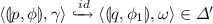
• 1. $id (B)= \{B\}$. This is the identity function.

• 2.
  

  This function checks whether all the environments are equal and returns $\{B_1\}$ (which is also equal to $B_i$ for every i). Otherwise, it returns the emptyset.

• 3.
  $$\begin{aligned}&meet^x_{\{c_1,..., c_n\}}(B_1,..., B_n)=\\&{\left\{ \begin{array}{ll} Abs_x(B_1) &{} \text {if } B_i(x) = c_i \text { for } 1 \le i \le n, \\ &{}\text { and } B_i(y) = B_j (y) \text { for } y \ne x, 1 \le i,j \le n; \\ \emptyset &{} \text {otherwise} \end{array}\right. }\\ \end{aligned}$$

  This function checks whether (1) $B_i(x) = c_i$ for every $1 \le i \le n$ (2) for every $y \ne x$; every $1 \le i, j \le n\,\,B_i(y) = B_j(y)$. If the conditions are satisfied, it returns $Abs_x(B_1)$¹, otherwise it returns the emptyset.

• 4.
  $$\begin{aligned}&join_c^{x} (B_1,..., B_n)= {\left\{ \begin{array}{ll} B_1 &{} \text {if } B_i(x) = c \text { for } 1 \le i \le n \\ &{} \text { and } B_i = B_j \text { for } 1 \le i,j \le n; \\ \emptyset &{} \text {otherwise} \end{array}\right. }\\ \end{aligned}$$

  This function checks whether $B_i(x) = c$ for every i. If this condition is satisfied, $equal(B_1,..., B_n)$ is returned, otherwise, the emptyset is returned.

• 5.
  $$\begin{aligned} join_c^{\lnot x} (B_1,..., B_n)= {\left\{ \begin{array}{ll}\\ B_1 &{} \text {if } B_i(x) \ne c \text { for } 1 \le i \le n \\ &{} \text { and } B_i = B_j \text { for } 1 \le i,j \le n; \\ \emptyset &{} \text {otherwise} \end{array}\right. } \end{aligned}$$

  This function checks whether $B_i(x) \ne c$ for every i. If this condition is satisfied, $equal(B_1,..., B_n)$ is returned, otherwise, the emptyset is returned.

4.3 From SBPCARET Model Checking of PDSs to the Membership Problem in SABPDSs

Let $\mathcal {P} = (P, \varGamma , \varDelta )$ be a PDS. We suppose w.l.o.g. that $\mathcal {P}$ has a bottom stack symbol $\sharp$ that is never popped from the stack. Let AP be a set of atomic propositions. Let $\varphi$ be a SBPCARET formula over AP, $\lambda : P \longrightarrow 2^{AP_\mathcal {D} }$ be a labelling function. Given a configuration $\langle p_0, \omega _0 \rangle$, we propose in this section an algorithm to check whether $\langle p_0, \omega _0 \rangle \vDash _{\lambda } \varphi$, i.e., whether there exists an environment B s.t. $\langle p_0, \omega _0 \rangle \vDash _{\lambda }^B \varphi$. Intuitively, we compute an SABPDS $\mathcal {BP}_\varphi$ s.t. $\langle p, \omega \rangle \vDash _{\lambda }^B \varphi$ iff for every $p \in P$, $\omega \in \varGamma ^*$, $B \in \mathcal {B}$. Then, to check if $\langle p_0, \omega _0 \rangle \vDash _{\lambda } \varphi$, we will check whether there exists a $B \in \mathcal {B}$ s.t. .

Let $Reg^+(\varphi ) = \{ e_1,..., e_k \}$ and $Reg^-(\varphi ) = \{ e_{k+1},..., e_m\}$. Using Theorems 1 and 2; for every $1 \le i \le k$, we can compute a VA $M_{e_i} = (Q_{e_i}, \varGamma , \delta _{e_i}, s_{e_i}, F_{e_i})$ s.t. $L(M_{e_i}) = L(e_i)$. In addition, for every $k+1 \le j \le m$, we can compute a VA $M_{\lnot e_j} = (Q_{\lnot e_j}, \varGamma , \delta _{\lnot e_j}, s_{\lnot e_j}, F_{\lnot e_j})$ s.t. $L(M_{\lnot e_j}) = (P \times \varGamma ^*) \times \mathcal {B} \setminus L(e_j)$. Let $\mathcal {M}$ be the union of all these automata, $\mathcal {S}$ and $\mathcal {F}$ be respectively the union of all states and final states of these automata.

Let $\mathcal {BP}_\varphi = (P', \varGamma ', \varDelta ', F)$ be the SABPDS defined as follows:

• $P' = P \cup (P \times Cl(\varphi )) \cup \mathcal {S} \cup \{ p_{\bot } \}$

• $\varGamma ' = \varGamma \cup (\varGamma \times Cl(\varphi )) \cup \{ \gamma _{\bot } \}$

• $F = F_1 \cup F_2 \cup F_3 \cup F_4$ where

• $F_3 = P \times Cl_{R} (\varphi ) \times \mathcal {B}$ where $Cl_{R} (\varphi )$ is the set of formulas of $Cl(\varphi )$ in the form $E [\varphi _1 R^v \varphi _2]$ or $A [\varphi _1 R^v \varphi _2]$ ($v \in \{g, a\}$)

• $F_4 = \mathcal {F} \times \mathcal {B}$

The transition relation $\varDelta '$ is the smallest set of transition rules defined as follows: For every $p \in P$, $\phi \in Cl(\varphi )$, $\gamma \in \varGamma$ and $t \in \{call, ret, int\}$:

• ($\varvec{\hbar }$1) If $\phi = b(\alpha _1,..., \alpha _n)$, then,

• ($\varvec{\hbar }$2) If $\phi = \lnot b(\alpha _1,..., \alpha _n)$, then,

• ($\varvec{\hbar }$3) If $\phi = \phi _1 \wedge \phi _2$, then,

• ($\varvec{\hbar }$4) If $\phi = \phi _1 \vee \phi _2$, then, and

• ($\varvec{\hbar }$5) If $\phi = \exists x \phi _1$, then, for every $c \in \mathcal {D}$

• ($\varvec{\hbar }$6) If $\phi = \forall x \phi _1$, then, where is repeated m times in the right-hand side, where m is the number of elements in $\mathcal {D}$

• ($\varvec{\hbar }$7) If $\phi = E X^g \phi _1$, then

  for every

• ($\varvec{\hbar }$8) If $\phi = A X^g \phi _1$, then,

  , where for every $1 \le i \le n$, and these transitions are all the transitions of $\varDelta$ that are in the form that have $\langle {p, \gamma }\rangle$ on the left hand side.

• ($\varvec{\hbar }$9) If $\phi = E X^a \phi _1$, then,

  • (a) for every

  • (b) for every

  • (c) for every

• ($\varvec{\hbar }$10) If $\phi = A X^a \phi _1$, then,

  , , where $\langle p_{\bot }, \gamma _{\bot } \rangle$ is repeated k times in the right-hand side s.t.:

  • (a) for every $1 \le i \le m$, and these transitions are all the transitions of $\varDelta$ that are in the form that have $\langle p, \gamma \rangle$ on the left hand side.

  • (b) for every $1 \le i \le n$, and these transitions are all the transitions of $\varDelta$ that are in the form that have $\langle p, \gamma \rangle$ on the left hand side.

  • (c) for every $1 \le i \le k$, and these transitions are all the transitions of $\varDelta$ that are in the form that have $\langle p, \gamma \rangle$ on the left hand side.

• ($\varvec{\hbar }$11) If $\phi = E [\phi _1 U^g \phi _2]$, then,

  • (a)

  • (b) for every

• ($\varvec{\hbar }$12) If $\phi = E [\phi _1 U^a \phi _2]$, then,

  • (a)

  • (b) for every

  • (c) for every

  • (d) for every

• ($\varvec{\hbar }$13) If $\phi = A [\phi _1 U^g \phi _2]$, then,

  • (a)

  • (b) where for every $1 \le i \le n$, and these transitions are all the transitions of $\varDelta$ that are in the form that have $\langle p, \gamma \rangle$ on the left hand side.

• ($\varvec{\hbar }$14) If $\phi = A [\phi _1 U^a \phi _2]$, then,

  • (a)

  • (b) ; , where $\langle p_{\bot }, \gamma _{\bot } \rangle$ is repeated k times in the right-hand side s.t.:

    • for every $1 \le i \le m$, and these transitions are all the transitions of $\varDelta$ that are in the form that have $\langle p, \gamma \rangle$ on the left hand side.

    • for every $1 \le i \le n$, and these transitions are all the transitions of $\varDelta$ that are in the form that have $\langle p, \gamma \rangle$ on the left hand side.

    • for every $1 \le i \le k$, and these transitions are all the transitions of $\varDelta$ that are in the form that have $\langle p, \gamma \rangle$ on the left hand side.

• ($\varvec{\hbar }$15) If $\phi = E [\phi _1 R^g \phi _2]$, then, we add to $\varDelta '$ the rule:

  • (a)

  • (b) for every

• ($\varvec{\hbar }$16) If $\phi = A [\phi _1 R^g \phi _2]$, then, we add to $\varDelta '$ the rule:

  • (a)

  • (b) where for every $1 \le i \le n$, and these transitions are all the transitions of $\varDelta$ that are in the form that have $\langle p, \gamma \rangle$ on the left hand side.

• ($\varvec{\hbar }$17) If $\phi = E [\phi _1 R^a \phi _2]$, then,

  • (a)

  • (b) for every

  • (c) for every

  • (d) for every

• ($\varvec{\hbar }$18) If $\phi = A [\phi _1 R^a \phi _2]$, then,

  • (a)

  • (b) ; , where $\langle p_{\bot }, \gamma _{\bot } \rangle$ is repeated k times in the right-hand side s.t.:

    • for every $1 \le i \le m$, and these transitions are all the transitions of $\varDelta$ that are in the form that have $\langle p, \gamma \rangle$ on the left hand side.

    • for every $1 \le i \le n$, and these transitions are all the transitions of $\varDelta$ that are in the form that have $\langle p, \gamma \rangle$ on the left hand side.

    • for every $1 \le i \le k$, and these transitions are all the transitions of $\varDelta$ that are in the form that have $\langle p, \gamma \rangle$ on the left hand side.

• ($\varvec{\hbar }$19) for every :

  • for every $\gamma '' \in \varGamma$, $\phi _1 \in Cl(\varphi )$

• ( $\varvec{\hbar }$ 20)

• ($\varvec{\hbar }$21) for every :

• ($\varvec{\hbar }$22) If $\phi = e$, e is a regular expression, then,

• ($\varvec{\hbar }$23) If $\phi = \lnot e$, e is a regular expression, then,

• ($\varvec{\hbar }$24) for every transition in $\mathcal {M}$: , where:

  • (a) $\mathbb {R} = equal$ iff $\alpha = \gamma$

  • (b) $\mathbb {R} = join_\gamma ^{x}$ iff $\alpha = x \in \mathcal {X}$

  • (c) $\mathbb {R} = join_\gamma ^{\lnot x}$ iff $\alpha = \lnot x$ and $x \in \mathcal {X}$

• ($\varvec{\hbar }$25) for every $q \in \mathcal {F}$,

Roughly speaking, the SABPDS $\mathcal {BP}_\varphi$ is a kind of product between $\mathcal {P}$ and the SBPCARET formula $\varphi$ which ensures that $\mathcal {BP}_\varphi$ has an accepting run from iff the configuration $\langle p, \omega \rangle$ satisfies $\varphi$ under the environment B. The form of the control locations of $\mathcal {BP}_\varphi$ is where $\phi \in Cl(\varphi )$, $B \in \mathcal {B}$. Let us explain the intuition behind our construction:

• If $\phi = b(\alpha _1,..., \alpha _n)$, then, for every $\omega \in \varGamma ^*$, $\langle p, \omega \rangle \vDash _\lambda ^B \phi$ iff $b(B(\alpha _1),..., B(\alpha _n)) \in \lambda (p)$. Thus, for such a B, $\mathcal {BP}_\varphi$ should have an accepting run from iff $b(B(\alpha _1),..., B(\alpha _n)) \in \lambda (p)$. This is ensured by the transition rules in ($\varvec{\hbar }$1) which add a loop at and the fact that (because it is in $F_1$). The function id in ($\varvec{\hbar }$1) ensures that the environments before and after are the same.

• If $\phi = \lnot b(\alpha _1,..., \alpha _n)$, then, for every $\omega \in \varGamma ^*$, $\langle p, \omega \rangle \vDash _\lambda ^B \phi$ iff $b(B(\alpha _1),..., B(\alpha _n)) \notin \lambda (p)$. Thus, for such a B, $\mathcal {BP}_\varphi$ should have an accepting run from iff $b(B(\alpha _1),..., B(\alpha _n)) \notin \lambda (p)$. This is ensured by the transition rules in ($\varvec{\hbar }$2) which add a loop at and the fact that (because it is in $F_2$). The function id in ($\varvec{\hbar }$2) ensures that the environments before and after are the same.

• If $\phi = \phi _1 \wedge \phi _2$, then, for every $\omega \in \varGamma ^*$, $\langle p, \omega \rangle \vDash _\lambda ^B \phi$ iff ($\langle p, \omega \rangle \vDash _\lambda ^B \phi _1$ and $\langle p, \omega \rangle \vDash _\lambda ^B \phi _2$). This is ensured by the transition rules in ($\varvec{\hbar }$3) stating that $\mathcal {BP}_\varphi$ has an accepting run from iff $\mathcal {BP}_\varphi$ has an accepting run from both and . ($\varvec{\hbar }$4) is similar to ($\varvec{\hbar }$3).

• If $\phi = \exists x \phi _1$, then, for every $\omega \in \varGamma ^*$, $\langle p, \omega \rangle \vDash _\lambda ^B \phi$ iff there exists $c \in \mathcal {D}$ s.t. $\langle p, \omega \rangle \vDash _\lambda ^{B[x \leftarrow c]} \phi _1$. This is ensured by the transition rules in ($\varvec{\hbar }$5) stating that $\mathcal {BP}_\varphi$ has an accepting run from iff there exists $c \in \mathcal {D}$ s.t. $\mathcal {BP}_\varphi$ has an accepting run from since $B \in meet^x_{\{c\}}(B[x \leftarrow c])$

• If $\phi = \forall x \phi _1$, then, for every $\omega \in \varGamma ^*$, $\langle p, \omega \rangle \vDash _\lambda ^B \phi$ iff for every $c \in \mathcal {D}$, $\langle p, \omega \rangle \vDash _\lambda ^{B[x \leftarrow c]} \phi _1$. This is ensured by the transition rules in ($\varvec{\hbar }$6) stating that $\mathcal {BP}_\varphi$ has an accepting run from iff for every $c \in \mathcal {D}$, $\mathcal {BP}_\varphi$ has an accepting run from since if $\mathcal {D} = \{c_1,..., c_m \}$, then, $B \in meet^x_{\mathcal {D}}(B[x \leftarrow c_1],..., B[x \leftarrow c_m])$

• If $\phi = EX^g \phi _1$, then, for every $\omega \in \varGamma ^*$, $\langle p, \omega \rangle \vDash _\lambda ^B \phi$ iff there exists an immediate successor $\langle p', \omega ' \rangle$ of $\langle p, \omega \rangle$ s.t. $\langle p', \omega ' \rangle \vDash _\lambda ^B \phi _1$. This is ensured by the transition rules in ($\varvec{\hbar }$7) stating that $\mathcal {BP}_\varphi$ has an accepting run from iff there exists an immediate successor $\langle p', \omega ' \rangle$ of $\langle p, \omega \rangle$ s.t. $\mathcal {BP}_\varphi$ has an accepting run from . ($\varvec{\hbar }$8) is similar to ($\varvec{\hbar }$7).

• If $\phi = E [\phi _1 U^g \phi _2]$, then, for every $\omega \in \varGamma ^*$, $\langle p, \omega \rangle \vDash _\lambda ^B \phi$ iff $\langle p, \omega \rangle \vDash _\lambda ^B \phi _2$ or ($\langle p, \omega \rangle \vDash _\lambda ^B \phi _1$ and there exists an immediate successor $\langle p', \omega ' \rangle$ of $\langle p, \omega \rangle$ s.t. $\langle p', \omega ' \rangle \vDash _\lambda ^B \phi$). This is ensured by the transition rules in ($\varvec{\hbar }$11) stating that $\mathcal {BP}_\varphi$ has an accepting run from iff $\mathcal {BP}_\varphi$ has an accepting run from (by the rules in ($\varvec{\hbar }$11)(a) or ($\mathcal {BP}_\varphi$ has an accepting run from both and where $\langle p', \omega ' \rangle$ is an immediate successor of $\langle p, \omega \rangle$) (by the rules in ($\varvec{\hbar }$11)(b)). ($\varvec{\hbar }$13) is similar to ($\varvec{\hbar }$11).

• If $\phi = E [\phi _1 R^g \phi _2]$, then, for every $\omega \in \varGamma ^*$, $\langle p, \omega \rangle \vDash _\lambda ^B \phi$ iff ($\langle p, \omega \rangle \vDash _\lambda ^B \phi _2$ and $\langle p, \omega \rangle \vDash _\lambda ^B \phi _1$) or ($\langle p, \omega \rangle \vDash _\lambda ^B \phi _2$ and there exists an immediate successor $\langle p', \omega ' \rangle$ of $\langle p, \omega \rangle$ s.t. $\langle p', \omega ' \rangle \vDash _\lambda ^B \phi$). This is ensured by the transition rules in ($\varvec{\hbar }$15) stating that $\mathcal {BP}_\varphi$ has an accepting run from iff $\mathcal {BP}_\varphi$ has an accepting run from both and (by the rules in ($\varvec{\hbar }$15)(a)); or $\mathcal {BP}_\varphi$ has an accepting run from both and where $\langle p', \omega ' \rangle$ is an immediate successor of $\langle p, \omega \rangle$ (by the rules in ($\varvec{\hbar }$15)(b)). In addition, for $R^g$ formulas, the stop condition is not required, i.e, for a formula $\phi _1 R^g \phi _2$ that is applied to a specific run, we don’t require that $\phi _1$ must eventually hold. To ensure that the runs on which $\phi _2$ always holds are accepted, we add to the Büchi accepting condition F (via the subset $F_3$ of F). ($\varvec{\hbar }$16) is similar to ($\varvec{\hbar }$15).

• If $\phi = EX^a \phi _1$, then, for every $\omega \in \varGamma ^*$, $\langle p, \omega \rangle \vDash _\lambda ^B \phi$ iff there exists an abstract-successor $\langle p_k, \omega _k \rangle$ of $\langle p, \omega \rangle$ s.t. $\langle p_k, \omega _k \rangle \vDash _\lambda ^B \phi _1$ (A1). Let $\uppi \in Traces(\langle p, \omega \rangle )$ be a run starting from $\langle p, \omega \rangle$ on which $\langle p_k, \omega _k \rangle$ is the abstract-successor of $\langle p, \omega \rangle$. Over $\uppi$, let $\langle p', \omega ' \rangle$ be the immediate successor of $\langle p, \omega \rangle$. In what follows, we explain how we can ensure this.

Fig. 2.

corresponds to a call statement

1. Firstly, we show that for every abstract-successor $\langle p_k, \omega _k \rangle \ne \bot$ of $\langle p, \omega \rangle$, where $B \in \mathcal {B}$. There are two possibilities:

• If corresponds to a call statement. Let us consider Fig. 2 to explain this case. is ensured by the rules in ($\varvec{\hbar }$9)(a), the rules in ($\varvec{\hbar }$21) and the rules in ($\varvec{\hbar }$19) as follows: rules in ($\varvec{\hbar }$9)(a) allow to record $\phi _1$ in the return point of the call, rules in ($\varvec{\hbar }$21) allow to mimic the run of the PDS $\mathcal {P}$ and rules in ($\varvec{\hbar }$19) allow to extract and put back $\phi _1$ when the return-point is reached. In what follows, we show in more details how this works: Let be the rule associated with the transition , then we have $\omega = \gamma \omega ''$ and $\omega ' = \gamma ' \gamma '' \omega ''$. Let be the transition that corresponds to the ret statement of this call on $\uppi$.Let then be the corresponding return rule. Then, we have necessarily $\omega _{k-1} = \beta \gamma '' \omega ''$, since as explained in Sect. 2, $\gamma ''$ is the return address of the call. After applying this rule, $\omega _{k} = \gamma '' \omega ''$. In other words, $\gamma ''$ will be the topmost stack symbol at the corresponding return point of the call. So, in order to ensure that , we proceed as follows: At the call , we encode the formula $\phi _1$ into $\gamma ''$ by the rule in ($\varvec{\hbar }$9)(a) stating that . This allows to record $\phi _1$ in the corresponding return point of the stack. After that, the rules in ($\varvec{\hbar }$21) allow $\mathcal {BP}_\varphi$ to mimic the run $\uppi$ of $\mathcal {P}$ from $\langle p', \omega ' \rangle$ till the corresponding return-point of this call, where is the topmost stack symbol. More specifically, the following sequence of $\mathcal {P}$: will be mimicked by the following sequence of $\mathcal {BP}_\varphi$: using the rules of ($\varvec{\hbar }$21). At the return-point, we extract $\phi _1$ from the stack and encode it into $p_k$ by adding the transition rules in ($\varvec{\hbar }$19) . Therefore, we obtain that . The property holds for this case.

• If corresponds to a simple statement. Then, the abstract successor of $\langle p, \omega \rangle$ is its immediate successor $\langle p', \omega ' \rangle$. Thus, we get that $\langle p_k, \omega _k \rangle = \langle p', \omega ' \rangle$. From the transition rules ($\varvec{\hbar }$9)(b), we get that . Therefore, . The property holds for this case.

2. Now, let us consider the case where $\langle p_k, \omega _k \rangle$, the abstract successor of $\langle p, \omega \rangle$, is $\bot$. This case occurs when corresponds to a return statement. Then, one abstract successor of $\langle p, \omega \rangle$ is $\bot$. Note that $\bot$ does not satisfy any formula, i.e., $\bot$ does not satisfy $\phi _1$. Therefore, from , we need to ensure that the path of $\mathcal {BP}_\varphi$ reflecting the possibility in (A1) that $\langle p_k, \omega _k \rangle \vDash _\lambda ^B \phi _1$ is not accepted. To do this, we exploit additional trap configurations. We use $p_{\bot }$ and $\gamma _{\bot }$ as trap control location and trap stack symbol to obtain these trap configurations. To be more specific, let be the rule associated with the transition , then we have $\omega = \gamma \omega ''$ and $\omega ' = \omega ''$. We add the transition rule in ($\varvec{\hbar }$9)(c) to allow . Since a run of $\mathcal {BP}_\varphi$ includes only infinite paths, we equip these trap configurations with self-loops by the transition rules in ($\varvec{\hbar }$20), i.e., . As a result, we obtain a corresponding path in $\mathcal {BP}_\varphi$: . Note that this path is not accepted by $\mathcal {BP}_\varphi$ because $\llbracket p_{\bot }, B \rrbracket \notin F$.

In summary, for every abstract-successor $\langle p_k, \omega _k \rangle$ of $\langle p, \omega \rangle$, if $\langle p_k, \omega _k \rangle \ne \bot$, then, ; otherwise which is not accepted by $\mathcal {BP}_\varphi$. Therefore, (A1) is ensured by the transition rules in ($\varvec{\hbar }$9) stating that $\mathcal {BP}_\varphi$ has an accepting run from iff there exists an abstract successor $\langle p_k, \omega _k \rangle$ of $\langle p, \omega \rangle$ s.t. $\mathcal {BP}_\varphi$ has an accepting run from .

• If $\phi = AX^a \phi _1$: this case is ensured by the transition rules in ($\varvec{\hbar }$10) together with ($\varvec{\hbar }$19) and ($\varvec{\hbar }$21). The intuition of ($\varvec{\hbar }$10) is similar to that of ($\varvec{\hbar }$9).

• If $\phi = E [\phi _1 U^a \phi _2]$, then, for every $\omega \in \varGamma ^*$, $\langle p, \omega \rangle \vDash _\lambda ^B \phi$ iff $\langle p, \omega \rangle \vDash _\lambda ^B \phi _2$ or ($\langle p, \omega \rangle \vDash _\lambda ^B \phi _1$ and there exists an abstract successor $\langle p_k, \omega _k \rangle$ of $\langle p, \omega \rangle$ s.t. $\langle p_k, \omega _k \rangle \vDash _\lambda ^B \phi$) (A2). Let $\uppi \in Traces(\langle p, \omega \rangle )$ be a run starting from $\langle p, \omega \rangle$ on which $\langle p_k, \omega _k \rangle$ is the abstract-successor of $\langle p, \omega \rangle$. Over $\uppi$, let $\langle p', \omega ' \rangle$ be the immediate successor of $\langle p, \omega \rangle$.

1. Firstly, we show that for every abstract-successor $\langle p_k, \omega _k \rangle \ne \bot$ of $\langle p, \omega \rangle$, where $B \in \mathcal {B}$. There are two possibilities:

• If corresponds to a call statement. From the rules in ($\varvec{\hbar }$12)(b), we get that where $\langle p', \omega ' \rangle$ is the immediate successor of $\langle p, \omega \rangle$. Thus, to ensure that , we only need to ensure that . As for the case $\phi = EX^a \phi _1$, is ensured by the rules in ($\varvec{\hbar }$21) and the rules in ($\varvec{\hbar }$19): rules in ($\varvec{\hbar }$21) allow to mimic the run of the PDS $\mathcal {P}$ before the return and rules in ($\varvec{\hbar }$19) allow to extract and put back $\phi _1$ when the return-point is reached.

• If corresponds to a simple statement. Then, the abstract successor of $\langle p, \omega \rangle$ is its immediate successor $\langle p', \omega ' \rangle$. Thus, we get that $\langle p_k, \omega _k \rangle = \langle p', \omega ' \rangle$. From the transition rules ($\varvec{\hbar }$12)(c), we get that . Therefore, . In other words, $\mathcal {BP}_\varphi$ has an accepting run from both and where $\langle p_k, \omega _k \rangle$ is an abstract successor of $\langle p, \omega \rangle$. The property holds for this case.

2. Now, let us consider the case where $\langle p_k, \omega _k \rangle = \bot$. As explained previously, this case occurs when corresponds to a return statement. Then, the abstract successor of $\langle p, \omega \rangle$ is $\bot$. Note that $\bot$ does not satisfy any formula, i.e., $\bot$ does not satisfy $\phi$. Therefore, from , we need to ensure that the path reflecting the possibility in (A2) that ($\langle p, \omega \rangle \vDash _\lambda ^B \phi _1$ and $\langle p_k, \omega _k \rangle \vDash _\lambda ^B \phi$) is not accepted by $\mathcal {BP}_\varphi$. This is ensured as for the case $\phi = EX^a \phi _1$ by the transition rules in ($\varvec{\hbar }$12)(d).

In summary, for every abstract-successor $\langle p_k, \omega _k \rangle$ of $\langle p, \omega \rangle$, if $\langle p_k, \omega _k \rangle \ne \bot$, then, ; otherwise which is not accepted by $\mathcal {BP}_\varphi$. Therefore, (A2) is ensured by the transition rules in ($\varvec{\hbar }$12) stating that $\mathcal {BP}_\varphi$ has an accepting run from iff $\mathcal {BP}_\varphi$ has an accepting run from ; or $\mathcal {BP}_\varphi$ has an accepting run from both and where $\langle p_k, \omega _k \rangle$ is an abstract successor of $\langle p, \omega \rangle$.

• The intuition behind the rules corresponding to the cases $\phi = A [\phi _1 U^a \phi _2]$, $\phi = A [\phi _1 R^a \phi _2]$ are similar to the previous case.

• If $\phi = e (e \in \mathcal {V})$. Given $p \in P$, $e \in \mathcal {V}$, $\omega \in \varGamma ^*$, we get that the SABPDS $\mathcal {BP}_\varphi$ should accept iff $(\langle p, \omega \rangle , B) \in L(M_e)$. To check whether $(\langle p, \omega \rangle , B) \in L(M_e)$, we let $\mathcal {BP}_\varphi$ go to state $s_e$, the initial state corresponding to p in $M_e$ by adding rules in ($\varvec{\hbar }$22); and then, from this state, we will check whether $\omega$ is accepted by $M_e$ under B. This is ensured by the transition rules in ($\varvec{\hbar }$24) and ($\varvec{\hbar }$25). ($\varvec{\hbar }$24) lets $\mathcal {BP}_\varphi$ mimic a run of $M_e$ on $\omega$ under B, which includes three possibilities:

• if $\mathcal {BP}_\varphi$ is in a state $\llbracket q, B \rrbracket$ with $\gamma$ on the top of the stack where $\gamma \in \varGamma$, and if is a transition rule in $M_e$, then, $\mathcal {BP}_\varphi$ will move to states $\llbracket q_1, B \rrbracket ,..., \llbracket q_n, B \rrbracket$ and pop $\gamma$ from its stack. Note that popping $\gamma$ allows us to check the rest of the word. This is ensured by the rules corresponding to ($\varvec{\hbar }$24)(a). Then function equal ensures that all these environments are the same.

• if $\mathcal {BP}_\varphi$ is in a state $\llbracket q, B \rrbracket$ with $\gamma$ on the top of the stack, and if is a transition rule in $M_e$ where $x \in \mathcal {X}$, then, $\mathcal {BP}_\varphi$ can mimic a run of $M_e$ under B iff $B(x) = \gamma$. If this condition is guaranteed, $\mathcal {BP}_\varphi$ will move to states $\llbracket q_1, B \rrbracket ,..., \llbracket q_n, B \rrbracket$ and pop $\gamma$ from its stack. Again, popping $\gamma$ allows us to check the rest of the word. This is ensured by the rules corresponding to ($\varvec{\hbar }$24)(b). Then function $join_\gamma ^{x}$ ensures that all these environments are the same B and $B(x) = \gamma$.

• Similar to ($\varvec{\hbar }$24)(b), ($\varvec{\hbar }$24)(c) deals with the cases where is a transition rule in $M_e$ where $x \in \mathcal {X}$.

In each VA $M_e$, a configuration is accepted if the run with the word $\omega$ reaches a final state in $F_e$; i.e., if $\mathcal {BP}_\varphi$ reaches a state $q \in F_e$ with an empty stack, i.e., with a stack containing the bottom stack symbol $\sharp$. Thus, we should add $F_e \times \mathcal {B}$ as a set of accepting control locations in $\mathcal {BP}_\varphi$. This is why $F_4$ is a set of accepting control locations. In addition, since $\mathcal {BP}_\varphi$ only recognizes infinite paths, ($\varvec{\hbar }$25) adds a loop on every configuration $\langle \llbracket q, B \rrbracket , \sharp \rangle$ where $q \in F_e$.

• If $\phi = \lnot e (e \in \mathcal {V})$. This case is ensured by the transition rules in ($\varvec{\hbar }$23), ($\varvec{\hbar }$24) and ($\varvec{\hbar }$25). The intuition behind this case is similar to the case $\phi = e$.

We can show that:

Theorem 4

Given a PDS $\mathcal {P} = (P, \varGamma , \varDelta )$, a set of atomic propositions AP, a labelling function $\lambda : AP_{\mathcal {D}} \rightarrow 2^{P}$ and a SBPCARET formula $\varphi$, we can compute an SABPDS $\mathcal {BP}_\varphi$ such that for every configuration $\langle p, \omega \rangle$, for every $B \in \mathcal {B}$, $\langle p, \omega \rangle \vDash _\lambda ^B \varphi$ iff $\mathcal {BP}_\varphi$ has an accepting run from the configuration .

5 Conclusion

In this paper, we present a new logic SBPCARET and show how it can precisely and succinctly specify malicious behaviors. We then propose an efficient algorithm for SBPCARET model-checking for PDSs. Our algorithm is based on reducing the model checking problem to the emptiness problem of Symbolic Alternating Büchi Pushdown Systems.

References

Alur, R., Etessami, K., Madhusudan, P.: A temporal logic of nested calls and returns. In: Jensen, K., Podelski, A. (eds.) TACAS 2004. LNCS, vol. 2988, pp. 467–481. Springer, Heidelberg (2004). https://doi.org/10.1007/978-3-540-24730-2_35
Bergeron, J., Debbabi, M., Desharnais, J., Erhioui, M.M., Lavoie, Y., Tawbi, N.: Static detection of malicious code in executable programs. Int. J. Req. Eng. 184–189, 79 (2001)
Christodorescu, M., Jha, S.: Static analysis of executables to detect malicious patterns. In: Proceedings of the 12th Conference on USENIX Security Symposium - Volume 12, SSYM 2003, Berkeley, CA, USA, p. 12. USENIX Association (2003)
Kinder, J., Katzenbeisser, S., Schallhart, C., Veith, H.: Detecting malicious code by model checking. In: Julisch, K., Kruegel, C. (eds.) DIMVA 2005. LNCS, vol. 3548, pp. 174–187. Springer, Heidelberg (2005). https://doi.org/10.1007/11506881_11
Lakhotia, A., Kumar, E.U., Venable, M.: A method for detecting obfuscated calls in malicious binaries. IEEE Trans. Softw. Eng. 31(11), 955–968 (2005)
Nguyen, H.-V., Touili, T.: CARET model checking for malware detection. In: SPIN 2017 (2017)
Nguyen, H.-V., Touili, T.: CARET model checking for pushdown systems. In: SAC 2017 (2017)
Nguyen, H.-V., Touili, T.: Branching temporal logic of calls and returns for pushdown systems. In: Furia, C.A., Winter, K. (eds.) IFM 2018. LNCS, vol. 11023, pp. 326–345. Springer, Cham (2018). https://doi.org/10.1007/978-3-319-98938-9_19
Schwoon, S.: Model-checking pushdown systems. Dissertation, Technische Universität München, München (2002)
Song, F., Touili, T.: Pushdown model checking for malware detection. In: Flanagan, C., König, B. (eds.) TACAS 2012. LNCS, vol. 7214, pp. 110–125. Springer, Heidelberg (2012). https://doi.org/10.1007/978-3-642-28756-5_9
Song, F., Touili, T.: Efficient malware detection using model-checking. In: Giannakopoulou, D., Méry, D. (eds.) FM 2012. LNCS, vol. 7436, pp. 418–433. Springer, Heidelberg (2012). https://doi.org/10.1007/978-3-642-32759-9_34
Song, F., Touili, T.: LTL model-checking for malware detection. In: Piterman, N., Smolka, S.A. (eds.) TACAS 2013. LNCS, vol. 7795, pp. 416–431. Springer, Heidelberg (2013). https://doi.org/10.1007/978-3-642-36742-7_29
Song, F., Touili, T.: PoMMaDe: pushdown model-checking for malware detection. In: SIGSOFT 2013 (2013)
Author information
Authors and Affiliations
Corresponding authors
Editor information
Editors and Affiliations
Rights and permissions
Copyright information
© 2019 Springer Nature Switzerland AG
About this paper
Cite this paper
Nguyen, HV., Touili, T. (2019). BCARET Model Checking for Malware Detection. In: Hierons, R., Mosbah, M. (eds) Theoretical Aspects of Computing – ICTAC 2019. ICTAC 2019. Lecture Notes in Computer Science(), vol 11884. Springer, Cham. https://doi.org/10.1007/978-3-030-32505-3_16
Download citation
DOI: https://doi.org/10.1007/978-3-030-32505-3_16
Published:
Publisher Name: Springer, Cham
Print ISBN: 978-3-030-32504-6
Online ISBN: 978-3-030-32505-3
eBook Packages: Computer ScienceComputer Science (R0)