Compositional Verification of Concurrent Systems by Combining Bisimulations

Abstract

One approach to verify a property expressed as a modal $\mu$-calculus formula on a system with several concurrent processes is to build the underlying state space compositionally (i.e., by minimizing and recomposing the state spaces of individual processes, keeping visible only the relevant actions occurring in the formula), and check the formula on the resulting state space. It was shown previously that, when checking the formulas of the $L_{\mu }^{ dsbr }$ fragment of $\mu$-calculus (consisting of weak modalities only), individual processes can be minimized modulo divergence-preserving branching (divbranching) bisimulation. In this paper, we refine this approach to handle formulas containing both strong and weak modalities, so as to enable a combined use of strong or divbranching bisimulation minimization on concurrent processes depending whether they contain or not the actions occurring in the strong modalities of the formula. We extend $L_{\mu }^{ dsbr }$ with strong modalities and show that the combined minimization approach preserves the truth value of formulas of the extended fragment. We implemented this approach on top of the CADP verification toolbox and demonstrated how it improves the capabilities of compositional verification on realistic examples of concurrent systems.

1 Introduction

We consider the problem of verifying a temporal logic property on a concurrent system $P_1\ ||\ ...\ ||\ P_n$ consisting of n processes composed in parallel. We work in the action-based setting, the property being specified as a formula $\varphi$ of the modal $\mu$-calculus ($L_{\mu }$) [18] and the processes $P_i$ being described in a language with process algebraic flavour. A well-known problem is the state-space explosion that happens when the system state space exceeds the available computer memory.

Compositional verification is a set of techniques and tools that have proven efficient to palliate state-space explosion in many situations [11]. These techniques may be either independent of the property, i.e., focus only on the construction of the system state space, such as compositional state space construction [14, 19, 22, 29, 31,32,33]. Alternatively, they may depend on the property, e.g., verification of the property on the full system is decomposed in the verification of properties on (expectedly smaller) sub-systems, such as in compositional reachability analysis [4, 36], assume-guarantee reasoning [28], or partial model checking [1].

Nevertheless, the frontier between property-independent and property-dependent techniques is loose. In compositional state space construction, to be able to reduce the system size, a set of actions is selected and a suitable equivalence relation (e.g., strong bisimulation, branching bisimulation, or divergence-preserving branching bisimulation—divbranching for short) is chosen, restricting the set of properties preserved after hiding the selected actions and reducing the system w.r.t. the selected relation. Therefore, there is still a dependency between the state space construction and the set of properties that can be verified. Given a formula $\varphi$ of $L_{\mu }$ to be verified on the system, Mateescu and Wijs [24] have pushed this idea and shown how to extract a maximal hiding set of actions and an equivalence relation (either strong or divbranching bisimulation) automatically from $\varphi$, thus inviting the compositional state space construction technique to the table of property-dependent reductions. To select the equivalence relation from the formula, they have identified an $L_{\mu }$ fragment named $L_{\mu }^{ dsbr }$, which is adequate with divbranching bisimulation [24]. This fragment consists of $L_{\mu }$ restricted to weak modalities, which match actions preceded by arbitrary sequences of hidden actions, as opposed to traditional strong modalities $\langle \alpha \rangle \,\varphi _0$ and $[\alpha ]\,\varphi _0$, which match only a single action satisfying $\alpha$. If $\varphi$ belongs to $L_{\mu }^{ dsbr }$, then the system can be reduced for divbranching bisimulation; otherwise, it can be reduced for strong bisimulation, the weakest equivalence relation preserving full $L_{\mu }$.

In this paper, we revisit and refine this approach to accommodate $L_{\mu }$ formulas containing both strong and weak modalities. To do so, we define a logic named $L_{\mu }^{ strong }(A_s)$, which extends $L_{\mu }^{ dsbr }$ with strong modalities matching only the actions belonging to a given set $A_s$ of strong actions. The set $A_s$ induces a partition of the processes $P_1\ ||\ ...\ ||\ P_n$ into those containing at least one strong action, and those that do not. We show that a formula $\varphi$ of $L_{\mu }^{ strong }(A_s)$ is still preserved if the processes containing strong actions are reduced modulo strong bisimulation and the other ones modulo divbranching bisimulation. We also provide guidelines for extracting the set $A_s$ from particular $L_{\mu }$ formulas encoding the operators of widely-used temporal logics, such as CTL [5], ACTL [26], PDL [9], and PDL-$\varDelta$ [30]. This combined use of bisimulations to reduce different parts of the same system makes possible a fine-tuning of the compositional state space construction by going smoothly from strong bisimulation (when all modalities are strong) to divbranching bisimulation (when $A_s$ is empty, as in the previous approach based on $L_{\mu }^{ dsbr }$). We implemented this approach on top of the CADP verification toolbox [12], and demonstrated how it improves the capabilities of compositional verification on two realistic case studies, namely the TFTP plane-ground communication protocol specified in [13] and the parallel CTL benchmark of the RERS’2018 challenge.

The paper is organized as follows. Section 2 recalls some definitions. Section 3 defines $L_{\mu }^{ strong }(A_s)$ and proves the main result of its adequacy with the combined use of strong and divbranching bisimulations. Section 4 presents the experimental results obtained on the two case studies. Finally, Sect. 5 contains concluding remarks and directions of future work. Formal proofs and code of case studies are available at https://doi.org/10.5281/zenodo.2634148.

2 Background

2.1 LTS Compositions and Reductions

We consider systems whose behavioural semantics can be represented using an LTS (Labelled Transition System).

Definition 1

(LTS). Let $\mathcal {A}$ denote an infinite set of actions, including the invisible action $\tau$, which denotes internal behaviour. All other actions are called visible. An LTS is a tuple $(\varSigma , A, {\mathop {\longrightarrow }\limits ^{}}, p_{ init })$, where $\varSigma$ is a set of states, $A \subseteq \mathcal {A}$ is a set of actions, ${\mathop {\longrightarrow }\limits ^{}}\ \subseteq \varSigma \times A \times \varSigma$ is the (labelled) transition relation, and $p_{ init } \in \varSigma$ is the initial state. We write $p {\mathop {\longrightarrow }\limits ^{a}} p'$ if $(p, a, p') \in \ {\mathop {\longrightarrow }\limits ^{}}$ and $p {\mathop {\longrightarrow }\limits ^{\tau ^*}} p'$ if there is a (possibly empty) sequence of $\tau$-transitions from p to $p'$, i.e., states $p_0, \ldots , p_n\ (n \ge 0)$ such that $p = p_0$, $p' = p_n$, and $p_i {\mathop {\longrightarrow }\limits ^{\tau }} p_{i+1}$ for $i = 0, \ldots , n-1$.

LTS can be composed in parallel and their actions can be abstracted away using the parallel composition and hiding operators defined below. Prior to hiding, an action mapping operator is also introduced for the generality of the approach.

Definition 2

(Parallel composition of LTS). Let $P = (\varSigma _P, A_P, {\mathop {\longrightarrow }\limits ^{}}_P, p_{ init })$, $Q = (\varSigma _Q, A_Q, {\mathop {\longrightarrow }\limits ^{}}_Q, q_{ init })$, and $A_{ sync } \subseteq \mathcal {A} \setminus \{\tau \}$. The parallel composition of P and Q with synchronization on $A_{ sync }$, “$P\ |[A_{ sync }]|\ Q$”, is defined as $(\varSigma _P \times \varSigma _Q, A_P \cup A_Q, {\mathop {\longrightarrow }\limits ^{}}, (p_{ init }, q_{ init }))$, where $(p, q) {\mathop {\longrightarrow }\limits ^{a}} (p', q')$ if and only if either (1) $p {\mathop {\longrightarrow }\limits ^{a}} p'$, $q' = q$, and $a \notin A_{ sync }$, or (2) $p' = p$, $q {\mathop {\longrightarrow }\limits ^{a}} q'$, and $a \notin A_{ sync }$, or (3) $p {\mathop {\longrightarrow }\limits ^{a}} p'$, $q {\mathop {\longrightarrow }\limits ^{a}} q'$, and $a \in A_{ sync }$.

Definition 3

(Action mapping). Let $P = (\varSigma _P, A_P, {\mathop {\longrightarrow }\limits ^{}}_P, p_{ init })$ and a total function $\rho : A_P \rightarrow 2^{\mathcal {A}}$. We write $\rho (A_P)$ for the image of $\rho$, defined by $\bigcup _{a\in A_P}\rho (a)$. We write $\rho (P)$ for the action mapping $\rho$ applied to P, defined as the LTS $(\varSigma _P, \rho (A_P), {\mathop {\longrightarrow }\limits ^{}}_P', p_{ init })$ where ${\mathop {\longrightarrow }\limits ^{}}_P'\,= \{(p, a', p') \mid p {\mathop {\longrightarrow }\limits ^{a}}_P p' \wedge a' \in \rho (a) \}$. An action mapping $\rho$ is admissible if $\tau \in A_P \implies \rho (\tau ) = \{\tau \}$.

Action mapping enables a single action a to be mapped onto the empty set of actions, onto a single action $a'$, or onto more than one actions $a_0', \ldots , a_{n+1}'$ ($n \ge 0$). In the first case, every transition labelled by a is removed. In the second case, a is renamed into $a'$. In the third case, every transition labelled by a is replaced by $n+2$ transitions with same source and target states, labelled by $a_0', \ldots , a_{n+1}'$. Action hiding is a special case of admissible action mapping.

Definition 4

(Action hiding). Let $P = (\varSigma _P, A_P, {\mathop {\longrightarrow }\limits ^{}}_P, p_{ init })$ and $A \subseteq \mathcal {A} \setminus \{\tau \}$. We write “$\mathbf{hide }\ A\ \mathbf{in }\ P$” for the LTS $\rho (P)$, where $\rho$ is the admissible action mapping defined by $(\forall a \in A_P \cap A)\ \rho (a) = \{\tau \}$ and $(\forall a \in A_P \setminus A)\ \rho (a) = \{a\}$.

Parallel composition and admissible action mapping subsume all abstraction and composition operators encodable as networks of LTS [7, 11, 20], such as the parallel composition, hiding, renaming, and cut (or restriction) operators of CCS [25], CSP [2], mCRL [15], LOTOS [16], E-LOTOS [17], and LNT [3], as well as synchronization vectors¹. In the sequel, we write $P_1\,||\,\ldots \,||\,P_n$ for any expression composing $P_1, \ldots , P_n$ using these operators. Given any partition of $P_1, \ldots , P_n$ into arbitrary subsets $\mathcal {P}_1$ and $\mathcal {P}_2$, it is always possible to rewrite $P_1\ ||\ \ldots \ ||\ P_n$ in the form $(||_{P_i\in \mathcal {P}_1}P_i)\ ||\ (||_{P_j\in \mathcal {P}_2}P_j)$, even for non-associative parallel composition operators (e.g., $|[\ldots ]|$), using appropriate action mappings².

LTS can be compared and reduced with respect to well-known bisimulation relations. In this paper, we consider strong bisimulation [27] and divbranching bisimulation, which itself derives from branching bisimulation [34, 35].

Definition 5

(Bisimulations). A strong bisimulation is a symmetric relation $R \subseteq \varSigma \times \varSigma$ such that if $(p_1, p_2) \in R$ then: for all $p_1 {\mathop {\longrightarrow }\limits ^{a}} p_1'$, there exists $p_2'$ such that $p_2 {\mathop {\longrightarrow }\limits ^{a}} p_2'$ and $(p_1', p_2') \in R$. A branching bisimulation is a symmetric relation $R \subseteq \varSigma \times \varSigma$ such that if $(p_1, p_2) \in R$ then: for all $p_1 {\mathop {\longrightarrow }\limits ^{a}} p_1'$, either $a = \tau$ and $(p_1', p_2) \in R$, or there exists a sequence $p_2 {\mathop {\longrightarrow }\limits ^{\tau ^*}} p_2' {\mathop {\longrightarrow }\limits ^{a}} p_2''$ such that $(p_1, p_2') \in R$ and $(p_1', p_2'') \in R$. A divergence-preserving branching bisimulation (divbranching bisimulation for short) is a branching bisimulation R such that if $(p_1^0, p_2^0) \in R$ and there is an infinite sequence $p_1^0 {\mathop {\longrightarrow }\limits ^{\tau }} p_1^1 {\mathop {\longrightarrow }\limits ^{\tau }} p_1^2 {\mathop {\longrightarrow }\limits ^{\tau }} \ldots$ with $(p_1^i, p_2^0) \in R$ for all $i \ge 0$, then there is an infinite sequence $p_2^0 {\mathop {\longrightarrow }\limits ^{\tau }} p_2^1 {\mathop {\longrightarrow }\limits ^{\tau }} p_2^2 {\mathop {\longrightarrow }\limits ^{\tau }} \ldots$ such that $(p_1^i, p_2^j) \in R$ for all $i, j \ge 0$. Two states $p_1$ and $p_2$ are strongly (resp. branching, divbranching) bisimilar, written $p_1 \sim p_2$ (resp. $p_1 \sim _{ br }p_2$, $p_1 \sim _{ dsbr }p_2$), if there exists a strong (resp. branching, divbranching) bisimulation R such that $(p_1, p_2) \in R$. Two LTS $P_1$ and $P_2$ are strongly (resp. branching, divbranching) bisimilar, written $P_1 \sim P_2$ (resp. $P_1 \sim _{ br }P_2$, $P_1 \sim _{ dsbr }P_2$), if their initial states are strongly (resp. branching, divbranching) bisimilar.

Strong, branching, and divbranching bisimulations are congruences for parallel composition and admissible action mapping. This allows reductions to be applied at any intermediate step during the state space construction, thus potentially reducing the overall cost of reduction. However, since processes may constrain each other by synchronization, composing LTS two by two following the algebraic structure of the composition expression and applying reduction after each composition can be orders of magnitude less efficient than other strategies in terms of the largest intermediate LTS. Finding an optimal strategy is difficult. One generally relies on heuristics to select a subset of LTS to compose at each step of the compositional reduction. In this paper, we will use the smart reduction heuristic [6, 11], which is implemented within the SVL [10] tool of CADP [12]. This heuristic tries to find an efficient composition order by analysing the synchronization and hiding structure of the composition expression.

2.2 Temporal Logics

Definition 6

(Modal $\varvec{\mu }$-calculus [18]). The modal $\mu$-calculus ($L_{\mu }$) is built from action formulas $\alpha$ and state formulas $\varphi$, whose syntax and semantics w.r.t. an LTS $P = (\varSigma , A, {\mathop {\longrightarrow }\limits ^{}}, p_{ init })$ are defined as follows:

where $X \in \mathcal{X}$ are propositional variables denoting sets of states, $\delta : \mathcal{X} \rightarrow 2^\varSigma$ is a context mapping propositional variables to sets of states, $[\,]$ is the empty context, $\delta [U/X]$ is the context identical to $\delta$ except for variable X, which is mapped to state set U, the functional ${\varPhi _0}_{P, \delta } : 2^\varSigma \rightarrow 2^\varSigma$ associated to the formula $\mu X . \varphi _0$ is defined as ${\varPhi _0}_{P, \delta } (U) = [\![\varphi _0]\!]_{P} \delta [U/X]$, and $\varPhi ^k$ means k-fold application. We write $P\,\models \,\varphi$ (read P satisfies $\varphi$) for $p_0 \in [\![\varphi ]\!]_{P}[\,]$.

Action formulas $\alpha$ are built from actions and boolean operators. State formulas $\varphi$ are built from boolean operators, the possibility modality $\langle \alpha \rangle \,\varphi _0$ denoting the states with an outgoing transition labeled by an action satisfying $\alpha$ and leading to a state satisfying $\varphi _0$, and the minimal fixed point operator $\mu X . \varphi _0$ denoting the least solution of the equation $X = \varphi _0$ interpreted over $2^\varSigma$.

The usual derived operators are defined as follows: boolean connectors $\mathsf {true}= \lnot \mathsf {false}$ and $\varphi _1 \wedge \varphi _2 = \lnot (\lnot \varphi _1 \vee \lnot \varphi _2)$; necessity modality $[\alpha ]\,\varphi _0 = \lnot \langle \alpha \rangle \,\lnot \varphi _0$; and maximal fixed point operator $\nu X . \varphi _0 = \lnot \mu X.\lnot \varphi _0[\lnot X/X]$, where $\varphi _0[\lnot X/X]$ is the syntactic substitution of X by $\lnot X$ in $\varphi _0$. Syntactically, $\langle \rangle \,$ and $[]\,$ have the highest precedence, followed by $\wedge$, then $\vee$, and finally $\mu$ and $\nu$. To have a well-defined semantics, state formulas are syntactically monotonic [18], i.e., in every subformula $\mu X . \varphi _0$, all occurrences of X in $\varphi _0$ fall in the scope of an even number of negations. Thus, negations can be eliminated by downward propagation.

Although $L_{\mu }$ subsumes most action-based logics, its operators are rather low-level and lead to complex formulas. In practice, temporal logics or extensions of $L_{\mu }$ with higher-level operators are used, avoiding (or at least reducing) the use of fixed point operators and modalities. We review informally some of these logics (whose operators can be translated to $L_{\mu }$), which will be useful in the sequel.

Propositional Dynamic Logic with Looping. The logic PDL-$\varDelta$ [30] introduces the modalities $\langle \beta \rangle \,\varphi _0$ and $\langle \beta \rangle \,@$, where $\beta$ is a regular formula defined as follows:

$$ \beta \,::\,= \varphi ? \mid \alpha \mid \beta _1 \cdot \beta _2 \mid \beta _1 \texttt {|} \beta _2 \mid \beta _0^* $$

Regular formulas $\beta$ denote sets of transition sequences in an LTS: the testing operator $\varphi ?$ denotes all zero-step sequences consisting of states satisfying $\varphi$; $\alpha$ denotes all one-step sequences consisting of a transition labeled by an action satisfying $\alpha$; the concatenation $\beta _1 \cdot \beta _2$, choice $\beta _1 \texttt {|} \beta _2$, and transitive-reflexive closure $\beta _0^*$ operators have their usual semantics transposed to transition sequences.

The regular diamond modality $\langle \beta \rangle \,\varphi _0$ denotes the states with an outgoing transition sequence satisfying $\beta$ and leading to a state satisfying $\varphi _0$. The infinite looping operator $\langle \beta \rangle \,@$ denotes the states having an outgoing transition sequence consisting of an infinite concatenation of subsequences satisfying $\beta$.

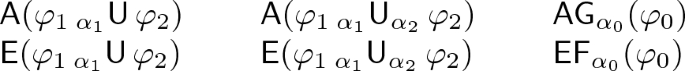
Action Computation Tree Logic. The logic ACTL$\setminus$X (ACTL without next operator) [26] introduces four temporal operators, whose semantics can be found in terms of $L_\mu$ formulas in [8, 24], where $\alpha _1, \alpha _2$ are interpreted over visible actions:

$$ \mathsf {E}(\varphi _1\,_{\alpha _1}\mathsf {U}\,\varphi _2), \mathsf {E}(\varphi _1\,_{\alpha _1}\mathsf {U}_{\alpha _2}\,\varphi _2), \mathsf {A}(\varphi _1\,_{\alpha _1}\mathsf {U}\,\varphi _2), \mathsf {A}(\varphi _1\,_{\alpha _1}\mathsf {U}_{\alpha _2}\,\varphi _2) $$

A transition sequence satisfies the path formula $\varphi _1\,_{\alpha _1}\mathsf {U}_{\alpha _2}\,\varphi _2$ if it contains a visible transition whose action satisfies $\alpha _2$ and whose target state satisfies $\varphi _2$, whereas at any moment before this transition, $\varphi _1$ holds and all visible actions satisfy $\alpha _1$. A sequence satisfies $\varphi _1\,_{\alpha _1}\mathsf {U}\,\varphi _2$ if it contains a state satisfying $\varphi _2$ and at any moment before, $\varphi _1$ holds and all visible actions satisfy $\alpha _1$. A state satisfies $\mathsf {E}(\varphi _1\,_{\alpha _1}\mathsf {U}_{\alpha _2}\,\varphi _2)$ (resp. $\mathsf {E}(\varphi _1\,_{\alpha _1}\mathsf {U}\,\varphi _2)$) if it has an outgoing sequence satisfying $\varphi _1\,_{\alpha _1}\mathsf {U}_{\alpha _2}\,\varphi _2$ (resp. $\varphi _1\,_{\alpha _1}\mathsf {U}\,\varphi _2$). It satisfies $\mathsf {A}(\varphi _1\,_{\alpha _1}\mathsf {U}_{\alpha _2}\,\varphi _2)$ (resp. $\mathsf {A}(\varphi _1\,_{\alpha _1}\mathsf {U}\,\varphi _2)$) if all its outgoing sequences satisfy the corresponding path formula. The following abbreviations are often used:

$$ \mathsf {EF}_{\alpha }(\varphi _0) = \mathsf {E}(\mathsf {true}\,_{\mathsf {true}}\mathsf {U}_{\alpha }\,\varphi _0) \qquad \mathsf {AG}_{\alpha }(\varphi _0) = \lnot \mathsf {EF}_{\lnot \alpha }(\mathsf {true}) \wedge \lnot \mathsf {E}(\mathsf {true}\,_{\mathsf {true}}\mathsf {U}\,\lnot \varphi _0) $$

A state satisfies $\mathsf {EF}_{\alpha }(\varphi _0)$ if it has an outgoing sequence leading to a transition whose action satisfies $\alpha$ and target state satisfies $\varphi _0$. A state satisfies $\mathsf {AG}_{\alpha }(\varphi _0)$ if none of its outgoing sequences leads to a transition labeled by an action not satisfying $\alpha$ or to a state not satisfying $\varphi _0$.

Computation Tree Logic. The logic CTL [5] contains the following operators:

$$ \mathsf {E}(\varphi _1\,\mathsf {U}\,\varphi _2), \mathsf {A}(\varphi _1\,\mathsf {U}\,\varphi _2), \mathsf {E}(\varphi _1\,\mathsf {W}\,\varphi _2), \mathsf {A}(\varphi _1\,\mathsf {W}\,\varphi _2), \mathsf {EF}(\varphi _0), \mathsf {AG}(\varphi _0), \mathsf {AF}(\varphi _0), \mathsf {EG}(\varphi _0) $$

A state satisfies $\mathsf {E}(\varphi _1\,\mathsf {U}\,\varphi _2)$ (resp. $\mathsf {A}(\varphi _1\,\mathsf {U}\,\varphi _2)$) if some of (resp. all) its outgoing sequences lead to states satisfying $\varphi _2$ after passing only through states satisfying $\varphi _1$. It satisfies $\mathsf {E}(\varphi _1\,\mathsf {W}\,\varphi _2)$ (resp. $\mathsf {A}(\varphi _1\,\mathsf {W}\,\varphi _2)$) if some of (resp. all) its outgoing sequences either contain only states satisfying $\varphi _1$, or lead to states satisfying $\varphi _2$ after passing only through states satisfying $\varphi _1$. A state satisfies $\mathsf {EF}(\varphi _0)$ (resp. $\mathsf {AF}(\varphi _0)$) if some of (resp. all) its outgoing sequences lead to states satisfying $\varphi _0$. A state satisfies $\mathsf {EG}(\varphi _0)$ (resp. $\mathsf {AG}(\varphi _0)$) if some of (resp. all) its outgoing sequences contain only states satisfying $\varphi _0$.

2.3 Compositional Property-Dependent LTS Reductions

Given a formula $\varphi \in L_{\mu }$ and a composition of processes $P_1\,||\,\ldots \,||\,P_n$, [24] shows two results that allow an LTS equivalent to $P_1\,||\,\ldots \,||\,P_n$ to be reduced compositionally, while preserving the truth value of $\varphi$. The first result is a procedure, called maximal hiding, which extracts systematically from $\varphi$ a set of actions $H(\varphi )$ that are not discriminated by any action formula occurring in $\varphi$. It is shown that $P_1\ ||\ \ldots \ ||\ P_n\,\models \,\varphi$ if and only if $\mathbf{hide }\ H(\varphi )\ \mathbf{in }\ (P_1\ ||\ \ldots \ ||\ P_n)\,\models \,\varphi$. The second result is the identification of a fragment of $L_{\mu }$, called $L_{\mu }^{ dsbr }$, which is strictly more expressive than $\mu$ACTL$\setminus$X³ and adequate with divbranching bisimulation. This fragment is defined as follows.

Definition 7

(Modal $\varvec{\mu }$-calculus fragment $\varvec{L_{\mu }^{ dsbr }}$ [24]). By convention, we use the symbols $\alpha _{\tau }$ and $\alpha _a$ to denote action formulas such that $\tau \in [\![\alpha _{\tau }]\!]_A$ and $\tau \notin [\![\alpha _a]\!]_A$. The fragment $L_{\mu }^{ dsbr }$ of $L_{\mu }$ is defined as the set of formulas that are semantically equivalent to some formula of the following language:

The ultra-weak modality $\langle (\varphi _1?.\alpha _{\tau })^*\rangle \,\varphi _2$, weak modality $\langle (\varphi _1?.\alpha _{\tau })^*.\varphi _1?.\alpha _a\rangle \,\varphi _2$, and weak infinite looping modality $\langle \varphi _1?.\alpha _{\tau }\rangle \,@$ are shorthand notations for the respective $L_{\mu }$ formulas $\mu X.\varphi _2 \vee (\varphi _1 \wedge \langle \alpha _{\tau }\rangle \,X)$, $\mu X.\varphi _1 \wedge (\langle \alpha _a\rangle \,\varphi _2 \vee \langle \alpha _{\tau }\rangle \,X)$, and $\nu X.\varphi _1 \wedge \langle \alpha _{\tau }\rangle \,X$. Derived operators are also defined as follows:

Depending on the $L_{\mu }$ fragment $\varphi$ belongs to, it is thus possible to determine whether the system can or cannot be reduced for divbranching bisimulation.

3 Combining Bisimulations Compositionally

The above approach is a mono-bisimulation approach: either the formula is in $L_{\mu }^{ dsbr }$ and then the system is entirely reduced for divbranching bisimulation, or it is not and then the system is entirely reduced for strong bisimulation. We show in this section that, even if the formula is not in $L_{\mu }^{ dsbr }$, it may still be possible to reduce some processes among the parallel processes $P_1,\ldots ,P_n$ for divbranching instead of strong bisimulation. This approach relies on the fact that, in general, an arbitrary temporal logic formula $\varphi$ may be rewritten in a form that contains both weak modalities, as those present in $L_{\mu }^{ dsbr }$, and non-weak modalities of $L_{\mu }$ (called strong modalities in this context).

To do so, we characterize a family of fragments of $L_{\mu }$, each of which is written $L_{\mu }^{ strong }(A_s)$, where $A_s$ is the set of actions that can be matched by strong modalities. We then prove that if $\varphi$ belongs to $L_{\mu }^{ strong }(A_s)$ and some process $P_i$ does not contain any action from the set $A_s$, then $P_i$ can be reduced for divbranching bisimulation. Throughout this section, we assume that the concurrent system $P_1\ ||\ \ldots \ ||\ P_n$ is fixed, and we write A for the set of actions occurring in the system.

3.1 The $L_{\mu }^{ strong }(A_s)$ Fragments of $L_{\mu }$

Definition 8

(${L_{\mu }^{ strong }(A_s)}$). Let $A_s \subseteq A$ be a fixed set of actions, called strong actions, and let $\alpha _s$ denote any action formula such that $[\![\alpha _s]\!]_A \subseteq A_s$, called a strong action formula. The fragment $L_{\mu }^{ strong }(A_s)$ of $L_{\mu }$ is defined as the set of formulas that are semantically equivalent to some formula of the following language:

We call $\langle \alpha _s\rangle \,\varphi _0$ a strong modality. $L_{\mu }^{ strong }(A_s)$ is the fragment of $L_{\mu }$ consisting of formulas expressible in a form where strong modalities match only actions in $A_s$. Its formal relationship with $L_{\mu }^{ dsbr }$ and $L_{\mu }$ is given in Theorem 1.

Theorem 1

The following three propositions hold trivially: $L_{\mu }^{ strong }(\emptyset ) = L_{\mu }^{ dsbr }$, $L_{\mu }^{ strong }(\mathcal {A}) = L_{\mu }$, and if $A_s \subset A_s'$ then $L_{\mu }^{ strong }(A_s) \subset L_{\mu }^{ strong }(A_s')$.

Given $\varphi \in L_{\mu }$, there exists a (not necessarily unique, see Theorem 3 page 10) minimal set $A_s$ such that $\varphi \in L_{\mu }^{ strong }(A_s)$. Obviously, $L_{\mu }^{ strong }(A_s)$ is not adequate with divbranching bisimulation when $A_s$ is not empty, as illustrated by the following example.

Fig. 1.

LTS used in Examples 1 and 2

Example 1

Consider the LTS P, $P'$, Q, and $Q'$ depicted in Fig. 1. $P'$ (resp. $Q'$) denotes the minimal LTS equivalent to P (resp. Q) for divbranching bisimulation. The formula $\varphi = [(\mathsf {true}?.\mathsf {true})^*.\mathsf {true}?.a_1]\,[a_2]\,\mathsf {false}$ of $L_{\mu }^{ strong }(\{a_2\})$ (which is equivalent to the PDL formula $[\mathsf {true}^*.a_1.a_2]\,\mathsf {false}$) expresses that the system does not contain two successive transitions labelled by $a_1$ and $a_2$ respectively. $\varphi$ does not belong to $L_{\mu }^{ dsbr }$. Indeed, $P\ |[a_1]|\ Q$ satisfies $\varphi$ because $a_1$ is necessarily followed by a $\tau$ transition, but $P'\ |[a_1]|\ Q'$ (which is isomorphic to $Q'$) does not.

3.2 Applying Divbranching Bisimulation to Selected Components

The following theorem states the main result of this paper, namely that every component process containing no strong action can be replaced by any divbranching equivalent process, without affecting the truth value of the formula⁴.

Theorem 2

Let $P = (\varSigma _P, A_P, \rightarrow _P, p_{ init })$, $Q = (\varSigma _Q, A_Q, {\mathop {\longrightarrow }\limits ^{}}_Q, q_{ init })$, $Q' = (\varSigma _{Q'}, A_{Q'}, {\mathop {\longrightarrow }\limits ^{}}_{Q'}, q_{ init }')$, $A_{ sync } \subseteq \mathcal {A}$, and $\varphi \in L_{\mu }^{ strong }(A_s)$. If $A_Q \cap A_s = \emptyset$ and $Q \sim _{ dsbr }Q'$, then $P\,|[A_{ sync }]|\,Q\,\models \,\varphi$ if and only if $P\,|[A_{ sync }]|\,Q'\,\models \,\varphi$.

Proof

The proof looks like the one in [24], showing that divbranching bisimulation preserves the properties of $L_{\mu }^{ dsbr }$, but reasoning concerns product states and additionally handles the case of strong modalities.    $\square$

Note that $\tau$ may belong to $A_s$. If so, every $P_i$ containing $\tau$ cannot be reduced for divbranching bisimulation. On the contrary, processes that do not contain strong actions do not contain $\tau$. Reducing them for divbranching bisimulation is thus allowed, but coincides with strong bisimulation reduction. In the end, all $\tau$-transitions of the system are preserved, as expected for the truth value of formulas containing strong modalities matching $\tau$ to be preserved.

Example 2

In Example 1, P does not contain $a_2$, the only strong action of the system. Thus, $\varphi$ can be checked on $P'\ |[a_1]|\ Q$ (which is isomorphic to Q and has only 3 states) instead of $P\ |[a_1]|\ Q$ (6 states), while preserving its truth value.

Theorem 2 is consistent with Andersen’s partial model checking [1] and the mono-bisimulation approach [24]. Given $P\,||\,Q$ such that the strong actions of $\varphi$ occur only in P, one can observe that the quotient $\varphi /\!/P$ (defined in [1, 21]) belongs to $L_{\mu }^{ dsbr }$, because quotienting removes all strong modalities, leaving only weak modalities in the quotiented formula. It follows that Q, on which $\varphi /\!/P$ has to be checked, can be reduced for divbranching bisimulation. This observation could serve as an alternative proof of Theorem 2.

3.3 Identifying Strong Actions in Derived Operators

In the general case, identifying a minimal set of strong actions is not easy, if even feasible. One cannot reasonably assume that formulas are written in the obscure $L_{\mu }^{ strong }(A_s)$ syntax (see Example 1) and that the remaining strong modalities cannot be turned to weak ones. Instead, users shall continue to use “syntactic sugar” extensions of $L_{\mu }$, with operators of e.g., CTL, ACTL, PDL, or PDL-$\varDelta$. In Lemma 1, we provide patterns that can be used to prove that a formula written using one of those operators belongs to a particular instance of $L_{\mu }^{ strong }(A_s)$.

Lemma 1

Let $\varphi _0, \varphi _1, \varphi _2 \in L_{\mu }^{ strong }(A_s)$, $\tau \in [\![\alpha _{\tau }]\!]_A$, $\tau \notin [\![\alpha _a]\!]_A$, $[\![\alpha _s]\!]_A \subseteq A_s$, and $\alpha _0, \alpha _1, \alpha _2$ be any action formulas. The following formulas belong to $L_{\mu }^{ strong }(A_s)$ (the list may be not exhaustive):

• 1. Modal $\varvec{\mu }$-calculus:

  

• 2. Propositional Dynamic Logic:

  

• 3. Action Computation Tree Logic:

  

• 4. Computation Tree Logic:

  

Example 3

Let $a_1$, $a_2$, and $a_3$ be visible actions and recall that A denotes the set of all actions of the system. Lemma 1 allows the following to be shown (this is left as an exercise):

Theorem 3

There is not a unique minimal set $A_s$ such that $\varphi \in L_{\mu }^{ strong }(A_s)$.

Proof

$\mathsf {EF}(\langle a_1\rangle \,\mathsf {true}\wedge \langle a_2\rangle \,\mathsf {true}) \in L_{\mu }^{ strong }(\{a_1\}) \cap L_{\mu }^{ strong }(\{a_2\})$, because it is semantically equivalent to both formulas $\mathsf {EF}(\langle (\langle a_1\rangle \,\mathsf {true}?.\mathsf {true})^*.\langle a_1\rangle \,\mathsf {true}?.a_2\rangle \,\mathsf {true})$ and $\mathsf {EF}(\langle (\langle a_2\rangle \,\mathsf {true}?.\mathsf {true})^*.\langle a_2\rangle \,\mathsf {true}?.a_1\rangle \,\mathsf {true})$. Yet, it is not in $L_{\mu }^{ strong }(\emptyset )$ as it has not the same truth value on the divbranching equivalent LTS P and $P'$ below:

Thus, $\{a_1\}$ and $\{a_2\}$ are non-unique minimal sets of strong actions.    $\square$

4 Applications

We consider two examples to illustrate our new verification approach combining strong and divbranching bisimulation and show how it can reduce both time and memory usage when associated to the smart reduction heuristic. In both examples, the aim is to perform a set of verification tasks, each consisting in checking a formula $\varphi$ on a system of parallel processes $P_1\ ||\ \ldots \ ||\ P_n$. Since our approach can only improve the verification of formulas containing both strong and weak modalities, we consider only the pairs of formulas and systems such that the formula is part of $L_{\mu }^{ strong }(A_s)$ for some minimal $A_s$ that is not empty and that is strictly included in the set of visible actions of the system⁵. For each verification task, we compare the largest LTS size, the verification time, and the memory peak obtained using the following two approaches:

• Mono-bisimulation approach: $\varphi$ is verified on $\mathbf{hide }\ H(\varphi )\ \mathbf{in }\ (P_1\ ||\ \ldots \ ||\ P_n)$ (where $H(\varphi )$ is the maximal hiding set mentioned in Sect. 2.3) reduced compositionally for strong bisimulation (since $\varphi$ is not in $L_{\mu }^{ dsbr }$) using the smart reduction heuristic.

• Refined approach combining bisimulations: The set $\{P_1, \ldots , P_n\}$ is partitioned in two groups $\mathcal {P}_s$ and $\mathcal {P}_w$ such that $P_i \in \mathcal {P}_s$ if it contains actions in $A_s$ and $P_i \in \mathcal {P}_w$ otherwise, so that $P_1\ ||\ \ldots \ ||\ P_n$ can be rewritten in the equivalent form $(||_{P_i\in \mathcal {P}_s}P_i)\ ||\ (||_{P_j\in \mathcal {P}_w}P_j)$. The set $A_I$ of actions on which at least one process of $\mathcal {P}_s$ and one process of $\mathcal {P}_w$ synchronize (inter-group synchronization) is then identified. Using the smart reduction heuristic, $\mathbf{hide }\ H(\varphi ) \setminus A_I\ \mathbf{in }\ ||_{P_i\in \mathcal {P}_s}P_i$ (corresponding to the processes containing strong actions) is reduced compositionally for strong bisimulation, leading to a first LTS $P_s$, and $\mathbf{hide }\ H(\varphi ) \setminus A_I\ \mathbf{in }\ ||_{P_j\in \mathcal {P}_w}P_j$ (corresponding to the processes containing no strong action) is reduced compositionally for divbranching bisimulation, leading to a second LTS $P_w$. Finally, $\varphi$ is verified on $\mathbf{hide }\ H(\varphi ) \cap A_I\ \mathbf{in }\ (P_s\ |[A_I]|\ P_w)$ reduced for strong bisimulation.

All experiments were done on a 3GHz/12GB RAM/8-core Intel Xeon computer running Linux, using the specification languages and 32-bit versions of tools provided in the CADP toolbox [12] version 2019-a “Pisa”.

4.1 Trivial File Transfer Protocol

The TFTP (Trivial File Transfer Protocol) case-study⁶ addresses the verification of an avionic communication protocol between a plane and the ground [13]. It comprises two instances (A and B) of a process named TFTP, connected through a FIFO buffer. Since the state space is very large in the general case, the authors defined five scenarios named A, B, C, D, and E, depending on whether each instance may write and/or read a file. The system corresponding to each scenario is a parallel composition of eight processes. The requirements consist of 29 properties parameterized by the identity of a TFTP instance, defined in MCL [23] (an implementation of the alternation-free modal $\mu$-calculus including PDL-$\varDelta$ modalities and macro definitions enabling the construction of libraries of operators), 24 of which belong to $L_{\mu }^{ dsbr }$. The remaining five, namely properties 08, 09, 14, 16, and 17, contain both weak and strong modalities. The shape of these properties is described in Table 1, where we do not provide the details of the action formulas, but instead denote them by letters $a_1, a_2, \ldots$, where $\tau \notin [\![a_i]\!]_A$ for all i. Strong action formulas are highlighted and one shows easily that the other are weak using Lemma 1-2.

Table 1. TFTP properties (strong action formulas are highlighted)

We consider 31 among a potential of 50 verification tasks (five properties, five scenarios, and two instances) as some properties are not relevant to every TFTP instance and scenario (e.g., in a scenario where one TFTP instance only receives messages, checking a property concerning a message emission is irrelevant). All 31 verification tasks return $\mathsf {true}$ and the strong actions occur in only three (although not the same three) out of the eight parallel processes.

Fig. 2.

Experimental results of the TFTP case-study

Figure 2 shows that the refined approach always reduces LTS size (for both intermediate and final LTS), memory and time following similar curves, up to a factor 7 (the vertical axis is on a logarithmic scale). Time does not include LTS generation of the component processes from their LNT specification, which takes only a few seconds and is common to both approaches. In these experiments, time is dominated by the last step of generation and minimization, whereas memory usage is dominated by minimization.

Table 2. RERS 2018 properties (strong action formulas are highlighted)

4.2 Parallel Benchmark of the RERS 2018 Challenge

The RERS (Rigorous Examination of Reactive Systems)⁷ challenge is an international competition on a benchmark of verification tasks. Since 2018 (8th edition), the challenge features a set of parallel problems where systems are synchronizing LTS and properties are expressed using CTL and modalities. This section illustrates the benefits of our approach on these problems.

The benchmark comprises three specifications of concurrent systems, numbered 101, 102, and 103, each accompanied by three properties to be checked, numbered p#21, p#22, and p#23, where p is the system number. Thus, nine verification tasks have to be solved. The properties are presented in Table 2, where the strong action formulas are highlighted. One easily shows that all other action formulas are weak using Lemmas 1-1 and 1-4. However, for 103#22 and 103#23, the identity $(\langle \alpha \rangle \,\mathsf {true}\Rightarrow [\alpha ]\,\varphi ) = ([\alpha ]\,\mathsf {false}\vee [\alpha ]\,\varphi ) = [\alpha ]\,\varphi$ (because $[\alpha ]\,\mathsf {false}\implies [\alpha ]\,\varphi$ for all $\varphi$) was applied to obtain the simplified formulas occurring after the $=$ sign in the table. For 102#23, this simplification allowed us to prove that A34 is not a strong action, unlike what appears at first sight.

Table 3. Some numbers about the RERS 2018 parallel benchmark

Table 3 gives, for each of the nine verification tasks, the number #act of actions in the system, the number #hide of actions in the maximal hiding set, the number #sact of strong actions, the number #proc of parallel processes, the number #sproc of processes in the strong group, the number #sync of inter-group actions, and the best reduction relation among strong bisimulation, divbranching bisimulation, or a combination of both. We observe that:

• The set of weak actions of 101#21 is empty due to the presence of the “$\mathsf {true}$” strong action formula, whereas the set of strong actions of 102#21 is empty, i.e., the property belongs to $L_{\mu }^{ dsbr }$. In both cases, our approach coincides with the mono-bisimulation approach. The verification of 101#21 (reduced for strong bisimulation) takes 75 s, with a memory peak of 11 MB and a largest LTS of 83, 964 states and 374, 809 transitions. The verification of 102#21 (reduced for divbranching bisimulation) takes 261 s, with a memory peak of 22 MB and a largest LTS of 243 states and 975 transitions.

• 101#22, 101#23, 102#22, 102#23, 103#21, 103#22, and 103#23 contain both weak and strong actions. They are used to evaluate our approach.

Table 4 compares the performance of verifying the latter seven verification tasks using the approaches described above. LTS sizes are given in kilostates, memory in megabytes, and time in seconds. Tasks using more than 3 GB of memory were aborted. We see that our approach reduces both time and memory usage and allows all problems of the challenge to be solved, whereas using strong bisimulation alone fails in five out of those seven tasks.

Table 4. Experimental results of the RERS 2018 parallel benchmark

The negligible reductions in time and memory usage observed for tasks 101#22 and 101#23 are due to the fact that time and memory usage are dominated by the algorithm in charge of selecting a sub-set of processes to be composed and reduced (implemented in smart reduction). The complexity of this algorithm does not depend on the state space size, but on the number of actions and parallel processes, which is almost the same using both approaches. When considering larger examples, memory usage gets dominated by minimisation. In particular, for tasks 102#22, 102#23, 103#21, and 103#23 (and likely also 103#22), memory usage is reduced by several orders of magnitude.

Note that some of these tasks can be verified more efficiently using non-compositional approaches, such as on-the-fly model checking, in cases where proofs or counter-examples can be detected much before having explored the full state space. The main drawback of maximal hiding is that the generated counter-examples are given only in terms of the actions visible in the formula, which abstracts out a lot of intermediate transitions. However, this is the price to pay for being able to verify most of the tasks, such as 103#21, for which on-the-fly verification aborts due to memory exhaustion.

5 Conclusion and Future Work

In this paper, we proposed a compositional verification approach that extends the state of the art [24] and consists of three steps: First, so-called strong actions are identified, corresponding to those actions of the system that the formula cannot match using weak modalities in the sense of the $L_{\mu }$ fragment $L_{\mu }^{ dsbr }$ adequate with divbranching bisimulation. These actions are used to partition the parallel processes into those containing strong actions and the others. Second, maximal hiding and compositional reduction are used to minimize the composition of processes not containing strong actions for divbranching bisimulation, and the other processes for strong bisimulation. Finally, the property is verified on the reduced system.

The originality of this approach is to combine strong and divbranching bisimulation, as opposed to the mono-bisimulation approach of [24]. We proved it correct by characterizing a family of fragments of the logic $L_{\mu }$, called $L_{\mu }^{ strong }(A_s)$, parameterized by the set $A_s$ of strong actions. We also showed under which conditions action-based branching-time temporal logic formulas containing well-known operators from the logics CTL, ACTL, PDL, and PDL-$\varDelta$ are part of $L_{\mu }^{ strong }(A_s)$ when $A_s$ is fixed. In the future, it might be worth investigating whether more operators can be considered, e.g., from the linear-time logic LTL.

This approach may significantly improve the verification performance for systems containing both processes with and without strong actions, as illustrated by two case-studies. In particular, it allowed the whole parallel CTL benchmark of the RERS 2018 challenge to be solved on a standard computer.

Identifying (close to minimal) sets of strong actions for arbitrary formulas manually is a cumbersome task, prone to errors. We shall investigate ways to compute such sets automatically. As illustrated by verification task 103#23 of RERS 2018, the problem is not purely syntactic: considering non-trivial semantic equivalences may prove useful to eliminate actions that appear strong at first sight. Yet, we trust that the presented approach has potential to be implemented in automated software tools, such as those available in the CADP toolbox.

References

Andersen, H.R.: Partial model checking. In: Proceedings of the 10th Annual IEEE Symposium on Logic in Computer Science LICS, San Diego, California, USA, pp. 398–407. IEEE Computer Society Press, June 1995
Brookes, S.D., Hoare, C.A.R., Roscoe, A.W.: A Theory of communicating sequential processes. J. ACM 31(3), 560–599 (1984)
Champelovier, D., et al.: Reference manual of the LNT to LOTOS translator (Version 6.7), INRIA, Grenoble, France, July 2017
Cheung, S.C., Kramer, J.: Enhancing compositional reachability analysis with context constraints. In: Proceedings of the 1st ACM SIGSOFT International Symposium on the Foundations of Software Engineering, Los Angeles, CA, USA, pp. 115–125. ACM Press, December 1993
Clarke, E.M., Emerson, E.A., Sistla, A.P.: Automatic verification of finite-state concurrent systems using temporal logic specifications. ACM Trans. Program. Lang. Syst. 8(2), 244–263 (1986)
Crouzen, P., Lang, F.: Smart reduction. In: Giannakopoulou, D., Orejas, F. (eds.) FASE 2011. LNCS, vol. 6603, pp. 111–126. Springer, Heidelberg (2011). https://doi.org/10.1007/978-3-642-19811-3_9
de Putter, S., Wijs, A., Lang, F.: Compositional Model Checking is Lively – Extended Version 2018. Submitted to Science of Computer Programming (2018)
Fantechi, A., Gnesi, S., Ristori, G.: From ACTL to \(\mu \)-calculus (extended abstract). In: Proceedings of the Workshop on Theory and Practice in Verification. ERCIM (1992)
Fischer, M.J., Ladner, R.E.: Propositional dynamic logic of regular programs. J. Comput. Syst. Sci. 18(2), 194–211 (1979)
Garavel, H., Lang, F.: SVL: a scripting language for compositional verification. In: Kim, M., Chin, B., Kang, S., Lee, D. (eds.) FORTE 2001. IFIP, vol. 69, pp. 377–392. Springer, Boston, MA (2002). https://doi.org/10.1007/0-306-47003-9_24
Garavel, H., Lang, F., Mateescu, R.: Compositional verification of asynchronous concurrent systems using CADP. Acta Informatica 52(4), 337–392 (2015)
Garavel, H., Lang, F., Mateescu, R., Serwe, W.: CADP 2011: a toolbox for the construction and analysis of distributed processes. Int. J. Softw. Tools Technol. Transf. (STTT) 15(2), 89–107 (2013)
Garavel, H., Thivolle, D.: Verification of GALS systems by combining synchronous languages and process calculi. In: Păsăreanu, C.S. (ed.) SPIN 2009. LNCS, vol. 5578, pp. 241–260. Springer, Heidelberg (2009). https://doi.org/10.1007/978-3-642-02652-2_20
Graf, S., Steffen, B.: Compositional minimization of finite state systems. In: Clarke, E.M., Kurshan, R.P. (eds.) CAV 1990. LNCS, vol. 531, pp. 186–196. Springer, Heidelberg (1991). https://doi.org/10.1007/BFb0023732
Groote, J.F., Ponse, A.: The Syntax and Semantics of \(\mu \)CRL. CS-R 9076. Centrum voor Wiskunde en Informatica, Amsterdam (1990)
ISO/IEC. LOTOS - A Formal Description Technique Based on the Temporal Ordering of Observational Behaviour. International Standard 8807, International Organization for Standardization - Information Processing Systems - Open Systems Interconnection, Geneva, September 1989
ISO/IEC. Enhancements to LOTOS (E-LOTOS). International Standard 15437:2001, International Organization for Standardization - Information Technology, Geneva, September 2001
Kozen, D.: Results on the propositional \(\mu \)-calculus. Theoret. Comput. Sci. 27, 333–354 (1983)
Krimm, J.-P., Mounier, L.: Compositional state space generation from Lotos programs. In: Brinksma, E. (ed.) TACAS 1997. LNCS, vol. 1217, pp. 239–258. Springer, Heidelberg (1997). https://doi.org/10.1007/BFb0035392
Lang, F.: Exp.Open 2.0: a flexible tool integrating partial order, compositional, and on-the-fly verification methods. In: Romijn, J., Smith, G., van de Pol, J. (eds.) IFM 2005. LNCS, vol. 3771, pp. 70–88. Springer, Heidelberg (2005). https://doi.org/10.1007/11589976_6
Lang, F., Mateescu, R.: Partial model checking using networks of labelled transition systems and boolean equation systems. Log. Methods Comput. Sci. 9(4), 1–32 (2013)
Malhotra, J., Smolka, S.A., Giacalone, A., Shapiro, R.: A tool for hierarchical design and simulation of concurrent systems. In: Proceedings of the BCS-FACS Workshop on Specification and Verification of Concurrent Systems, Stirling, Scotland, UK, pp. 140–152. British Computer Society, July 1988
Mateescu, R., Thivolle, D.: A model checking language for concurrent value-passing systems. In: Cuellar, J., Maibaum, T., Sere, K. (eds.) FM 2008. LNCS, vol. 5014, pp. 148–164. Springer, Heidelberg (2008). https://doi.org/10.1007/978-3-540-68237-0_12
Mateescu, R., Wijs, A.: Property-dependent reductions adequate with divergence-sensitive branching bisimilarity. Sci. Comput. Program. 96(3), 354–376 (2014)
Milner, R.: Communication and Concurrency. Prentice-Hall, Upper Saddle River (1989)
De Nicola, R., Vaandrager, F.: Action versus state based logics for transition systems. In: Guessarian, I. (ed.) LITP 1990. LNCS, vol. 469, pp. 407–419. Springer, Heidelberg (1990). https://doi.org/10.1007/3-540-53479-2_17
Park, D.: Concurrency and automata on infinite sequences. In: Deussen, P. (ed.) GI-TCS 1981. LNCS, vol. 104, pp. 167–183. Springer, Heidelberg (1981). https://doi.org/10.1007/BFb0017309
Pnueli, A.: In transition from global to modular temporal reasoning about programs. Log. Models Concurr. Syst. 13, 123–144 (1984)
Sabnani, K.K., Lapone, A.M., Ümit Uyar, M.: An algorithmic procedure for checking safety properties of protocols. IEEE Trans. Commun. 37(9), 940–948 (1989)
Streett, R.: Propositional dynamic logic of looping and converse. Inf. Control 54, 121–141 (1982)
Tai, K.-C., Koppol, P.V.: An incremental approach to reachability analysis of distributed programs. In: Proceedings of the 7th International Workshop on Software Specification and Design, Los Angeles, CA, USA, pp. 141–150, Piscataway, NJ, December 1993. IEEE Press (1993)
Tai, K.-C., Koppol, P.V.: Hierarchy-based incremental reachability analysis of communication protocols. In: Proceedings of the IEEE International Conference on Network Protocols, San Francisco, CA, USA, pp. 318–325. IEEE Press, Piscataway, NJ, October 1993 (1993)
Valmari, A.: Compositional state space generation. In: Rozenberg, G. (ed.) ICATPN 1991. LNCS, vol. 674, pp. 427–457. Springer, Heidelberg (1993). https://doi.org/10.1007/3-540-56689-9_54
van Glabbeek, R.J., Weijland, W.P.: Branching-time and abstraction in bisimulation semantics (extended abstract). CS R8911, Centrum voor Wiskunde en Informatica, Amsterdam 1989. Also in Proceedings IFIP 11th World Computer Congress, San Francisco (1989)
van Glabbeek, R.J., Weijland, W.P.: Branching time and abstraction in bisimulation semantics. J. ACM 43(3), 555–600 (1996)
Yeh, W.J., Young, M.: Compositional reachability analysis using process algebra. In: Proceedings of the ACM SIGSOFT Symposium on Testing, Analysis, and Verification (SIGSOFT 1991), Victoria, British Columbia, Canada, pp. 49–59. ACM Press, October 1991 (1991)
Author information
Authors and Affiliations
Corresponding author
Editor information
Editors and Affiliations
Rights and permissions
Copyright information
© 2019 Springer Nature Switzerland AG
About this paper
Cite this paper
Lang, F., Mateescu, R., Mazzanti, F. (2019). Compositional Verification of Concurrent Systems by Combining Bisimulations. In: ter Beek, M., McIver, A., Oliveira, J. (eds) Formal Methods – The Next 30 Years. FM 2019. Lecture Notes in Computer Science(), vol 11800. Springer, Cham. https://doi.org/10.1007/978-3-030-30942-8_13
Download citation
DOI: https://doi.org/10.1007/978-3-030-30942-8_13
Published:
Publisher Name: Springer, Cham
Print ISBN: 978-3-030-30941-1
Online ISBN: 978-3-030-30942-8
eBook Packages: Computer ScienceComputer Science (R0)