Counting Independent Sets in Graphs with Bounded Bipartite Pathwidth

Abstract

The Glauber dynamics can efficiently sample independent sets almost uniformly at random in polynomial time for graphs in a certain class. The class is determined by boundedness of a new graph parameter called bipartite pathwidth. This result, which we prove for the more general hardcore distribution with fugacity $\lambda$, can be viewed as a strong generalisation of Jerrum and Sinclair’s work on approximately counting matchings. The class of graphs with bounded bipartite pathwidth includes line graphs and claw-free graphs, which generalise line graphs. We consider two further generalisations of claw-free graphs and prove that these classes have bounded bipartite pathwidth.

M. Dyer and H. Müller—Research supported by EPSRC grant EP/S016562/1.

C. Greenhill—Research supported by Australian Research Council grant DP19010097.

1 Introduction

We will show that we can approximate the number of independent sets in graphs for which all bipartite induced subgraphs are well structured, in a sense that we will define precisely. Our approach is to generalise the Markov chain analysis of Jerrum and Sinclair [19] for the corresponding problem of counting matchings. Their canonical path argument relied on the fact that the symmetric difference of two matchings of a given graph G is a bipartite subgraph of G consisting of a disjoint union of paths and even-length cycles. We introduce a new graph parameter, which we call bipartite pathwidth, to enable us to give the strongest generalisation of the approach of [19].

1.1 Independent Set Problems

For a given graph G, let $\mathcal {I}(G)$ be the set of all independent sets in G. The independence number $\alpha (G) = \max \{|I| \, :\, I \in \mathcal {I}(G)\}$ is the size of the largest independent set in G. The problem of finding $\alpha (G)$ is NP-hard in general, even in various restricted cases, such as degree-bounded graphs. However, polynomial time algorithms have been constructed for finding a maximum independent set, for various graph classes. The most important case has been matchings, which are independent sets in the line graph L(G) of G. This has been generalised to larger classes of graphs, for example claw-free graphs [24], which include line graphs [4], and fork-free graphs [1], which include claw-free graphs.

Counting independent sets in graphs is known to be #P-complete in general [26], and in various restricted cases [15, 30]. Exact counting is known only for some restricted graph classes. Even approximate counting is NP-hard in general, and is unlikely to be in polynomial time for bipartite graphs [11].

For some classes of graphs, for example line graphs, approximate counting is known to be possible [19, 20]. The most successful Markov chain approach relies on a close correspondence between approximate counting and sampling uniformly at random [21]. It was applied to degree-bounded graphs in [23] and [12]. In his PhD thesis [22], Matthews used a Markov chain for sampling independent sets in claw-free graphs. His chain, and its analysis, generalises that of [19].

Several other approaches to approximate counting have been successfully applied to the independent set problem. Weitz [31] used the correlation decay approach on degree-bounded graphs, resulting in an FPTAS for counting independent sets in graphs with degree at most 5. Sly [29] gave a matching NP-hardness result. The correlation decay method was also applied to matchings in [3], and was extended to complex values of $\lambda$ in [16]. Recently, Efthymiou et  al. [14] proved that the Markov chain approach can (almost) produce the best results obtainable by other methods.

The independence polynomial $P_G(\lambda )$ of a graph G is defined in (1) below. The Taylor series approach of Barvinok [2] was used by Patel and Regts [25] to give a FPTAS for $P_G(\lambda )$ in degree-bounded claw-free graphs. The success of the method depends on the location of the roots of the independence polynomial. Chudnovsky and Seymour [7] proved that all these roots are real, and hence they are all negative. Then the algorithm of [25] is valid for all complex $\lambda$ which are not real and negative. In this extended abstract (for proofs see [13]), we return to the Markov chain approach.

1.2 Preliminaries

We write $[m] = \{1,2,\ldots , m\}$ for any positive integer m, and let $A\oplus B$ denote the symmetric difference of sets A, B. For graph theoretic definitions not given here, see [10]. Throughout this paper, all graphs are simple and undirected. G[S] denotes the subgraph of G induced by the set S and N(v) denotes the neighbourhood of vertex v. Given a graph $G=(V,E)$, let $\mathcal {I}_k(G)$ be the set of independent sets of G of size k. The independence polynomial of G is the partition function

$$\begin{aligned} P_G(\lambda )=\sum _{I\in \mathcal {I}(G)}\lambda ^{|I|}=\sum _{k=0}^{\alpha (G)} N_k\, \lambda ^k, \end{aligned}$$

(1)

where $N_k=|\mathcal {I}_k(G)|$ for $k=0,\ldots , \alpha$. Here $\lambda \in \mathbb {C}$ is called the fugacity. We consider only real $\lambda$ and assume $\lambda \ge 1/n$ to avoid trivialities. We have $N_0=1$, $N_1=n$ and $N_k\le \left( {\begin{array}{c}n\\ k\end{array}}\right)$ for $k=2,\ldots , n$. Thus it follows that for any $\lambda \ge 0$,

$$\begin{aligned} 1+n\lambda \le P_G(\lambda )\le \sum _{k=0}^{\alpha (G)} \left( {\begin{array}{c}n\\ k\end{array}}\right) \, \lambda ^k\le (1+\lambda )^n. \end{aligned}$$

(2)

Note also that $P_G(0)=1$ and $P_G(1)=|\mathcal {I}(G)|$.

An almost uniform sampler for a probability distribution $\pi$ on a state $\varOmega$ is a randomised algorithm which takes as input a real number $\delta > 0$ and outputs a sample from a distribution $\mu$ such that the total variation distance $\frac{1}{2}\sum _{x\in \varOmega }|\mu (x)-\pi (x)|$ is at most $\delta$. The sampler is a fully polynomial almost uniform sampler (FPAUS) if its running time is polynomial in the input size n and $\log (1/\delta )$. The word “uniform” here is historical, as it was first used in the case where $\pi$ is the uniform distribution. We use it in a more general setting.

If $w:\varOmega \rightarrow \mathbb {R}$ is a weight function, then the Gibbs distribution $\pi$ satisfies $\pi (x)=w(x)/W$ for all $x\in \varOmega$, where $W=\sum _{x\in \varOmega }w(x)$. If $w(x)=1$ for all $x\in \varOmega$ then $\pi$ is uniform. For independent sets with $w(I)=\lambda ^{|I|}$, we have

$$\begin{aligned} \pi (I) = \lambda ^{|I|}/P_G(\lambda ), \end{aligned}$$

(3)

and is often called the hardcore distribution. Jerrum, Valiant and Vazirani [21] showed that approximating W is equivalent to the existence of an FPAUS for $\pi$, provided the problem is self-reducible. Counting independent sets in a graph is a self-reducible problem. (2) can be tightened to

$$\begin{aligned} P_G(\lambda )\,\le \, \sum _{k=0}^\alpha \left( {\begin{array}{c}n\\ k\end{array}}\right) \, \lambda ^k\,\le \, \sum _{k=0}^\alpha \frac{(n\lambda )^k}{k!} \,\le \, (n\lambda )^\alpha \sum _{k=0}^\alpha \frac{1}{k!}\,\le \,e(n\lambda )^\alpha . \end{aligned}$$

(4)

2 Markov Chains

2.1 Mixing Time

For general information on Markov chains and approximate counting see [17, 18].

Consider a Markov chain on state space $\varOmega$ with stationary distribution $\pi$ and transition matrix $\mathbf {P}$. Let $p_n$ be the distribution of the chain after n steps. We will assume that $p_0$ is the distribution which assigns probability 1 to a fixed initial state $x\in \varOmega$. The mixing time of the Markov chain, from initial state $x\in \varOmega$, is $\tau _x(\varepsilon )= \min \{n : \text {d}_{\text {TV}}(p_n,\pi )\le \varepsilon \}$, where $\text {d}_{\text {TV}}(p_n,\pi )$ is the total variation distance between $p_n$ and $\pi$. In the case of the Glauber dynamics for independent sets, the stationary distribution $\pi$ satisfies (3), and in particular $\pi (\varnothing )^{-1}=P_G(\lambda )$. We will always use $\varnothing$ as our starting state.

Let $\beta _{\max } = \max \{\beta _1,|\beta _{|\varOmega |-1}|\}$, where $\beta _1$ is the second-largest eigenvalue and $\beta _{|\varOmega |-1}$ is the smallest eigenvalue of $\mathbf {P}$. From [9, Proposition 3] follows $\tau _{x}(\varepsilon ) \le (1-\beta _{\max })^{-1}\, \left( \ln (\pi (x)^{-1}) + \ln (1/\varepsilon )\right) ,$ see also [28, Proposition 1(i)]. Hence for $\lambda \ge 1/n$,

$$\begin{aligned} \tau _{\varnothing }(\varepsilon ) \le (1-\beta _{\max })^{-1}\, \left( \alpha (G)\ln (n\lambda ) + 1 + \ln (1/\varepsilon )\right) , \end{aligned}$$

(5)

using (4). We can easily prove that $(1+\beta _{|\varOmega |-1})^{-1}$ is bounded above by $\min \{\lambda , n\}$, see (9). It is more difficult to bound the relaxation time $(1-\beta _1)^{-1}$.

2.2 Canonical Paths Method

To bound the mixing time of our Markov chain we will apply the canonical paths method of Jerrum and Sinclair [19]. This may be summarised as follows. Let the problem size be n (in our setting, n is the number of vertices in the graph G, $\varOmega =\mathcal {I}(G)$ and hence $|\varOmega |\le 2^n$). For each pair of states $X, Y\in \varOmega$ we define a path $\gamma _{XY}$ from X to Y, namely $X=Z_0\rightarrow Z_2\rightarrow \cdots \rightarrow Z_\ell =Y$ such that successive pairs along the path are given by a transition of the Markov chain. Write $\ell _{XY}=\ell$ for the length of the path $\gamma _{XY}$, and let . We require to be at most polynomial in n. This is usually easy to achieve, but the set of paths $\{\gamma _{XY}\}$ must also satisfy the following property.

For any transition $(Z,Z')$ of the chain there must exist an encoding W, such that, given $(Z,Z')$ and W, there are at most $\nu$ distinct possibilities for X and Y such that $(Z,Z')\in \gamma _{XY}$. That is, each transition of the chain can lie on at most $\nu \, |\varOmega ^*|$ canonical paths, where $\varOmega ^*$ is some set which contains all possible encodings. We usually require $\nu$ to be polynomial in n. It is common to refer to the additional information provided by $\nu$ as “guesses”, and we will do so here. In our situation, all encodings will be independent sets, so we may assume that $\varOmega ^*=\varOmega$. The congestion $\varrho$ of the chosen set of paths is given by

$$\begin{aligned} \varrho =\max _{(Z,Z')}\bigg \{\frac{1}{\pi (Z)\mathbf {P}(Z,Z')} \sum _{X,Y:\gamma _{XY}\ni (Z,Z')}\pi (X)\pi (Y)\,\bigg \}, \end{aligned}$$

(6)

where the maximum is taken over all pairs $(Z,Z')$ with $\mathbf {P}(Z,Z')>0$ and $Z'\ne Z$ (that is, over all transitions of the chain), and the sum is over all paths containing the transition $(Z,Z')$. A bound on the relaxation time $(1-\beta _1)^{-1}$ will follow from a bound on congestion, using Sinclair’s result [28, Cor. 6]:

(7)

2.3 Glauber Dynamics

The Markov chain we employ will be the Glauber dynamics. In fact, we will consider a weighted version of this chain, for a given value of the fugacity (also called activity) $\lambda >0$. Define $\pi (Z) = \lambda ^{|Z|}/P_G(\lambda )$ for all $Z\in \mathcal {I}(G)$, where $P_G(\lambda )$ is the independence polynomial defined in (1). A transition from $Z\in \mathcal {I}(G)$ to $Z'\in \mathcal {I}(G)$ will be as follows. Choose a vertex v of G uniformly at random.

• If $v\in Z$ then $Z'\leftarrow Z{\setminus }\{v\}$ with probability $1/(1+\lambda )$.

• If $v\notin Z$ and $Z\cup \{v\}\in \mathcal {I}(G)$ then $Z'\leftarrow Z\cup \{v\}$ with probability $\lambda /(1+\lambda )$.

• Otherwise $Z'\leftarrow Z$.

This Markov chain is irreducible and aperiodic, and satisfies the detailed balance equations $\pi (Z)\, \mathbf {P}(Z,Z')=\pi (Z')\, \mathbf {P}(Z',Z)$ for all $Z,Z'\in \mathcal {I}(G)$. Therefore, the Gibbs distribution $\pi$ is the stationary distribution of the chain. If $Z'$ is obtained from Z by deleting a vertex v then

$$\begin{aligned} \mathbf {P}(Z,Z')=\frac{1}{n(1+\lambda )} \quad \text { and } \quad \mathbf {P}(Z',Z)=\frac{\lambda }{n(1+\lambda )}. \end{aligned}$$

(8)

The unweighted version is given by setting $\lambda =1$, and has uniform stationary distribution. Since the analysis for general $\lambda$ is hardly any more complicated than that for $\lambda =1$, we will work with the weighted case.

It follows from the transition procedure that $\mathbf {P}(Z,Z)\ge \min \{1,\lambda \}/(1+\lambda )$ for all states $Z\in \mathcal {I}(G)$. That is, every state has a self-loop probability of at least this value. Using a result of Diaconis and Saloff-Coste [8, p. 702], we conclude that the smallest eigenvalue $\beta _{|\mathcal {I}(G)|-1}$ of $\mathbf {P}$ satisfies

$$\begin{aligned} (1+\beta _{|\mathcal {I}(G)|-1})^{-1} \le \frac{1+\lambda }{2\min \{1,\lambda \}} \le \min \{\lambda , n\} \end{aligned}$$

(9)

for $\lambda \ge 1/n$. This bound will be dominated by our bound on the relaxation time. We will always use the initial state $Z_0=\varnothing$, since $\varnothing \in \mathcal {I}(G)$ for any graph G.

In order to bound the relaxation time $(1-\beta _1)^{-1}$ we will use the canonical path method. A key observation is that for any $X,Y\in \mathcal {I}(G)$, the induced subgraph $G[X\oplus Y]$ of G is bipartite. This can easily be seen by colouring vertices in $X{\setminus } Y$ black and vertices in $Y{\setminus } X$ white, and observing that no edge in G can connect vertices of the same colour. To exploit this observation, we introduce the bipartite pathwidth of a graph in Sect. 3. In Sect. 4 we show how to use the bipartite pathwidth to construct canonical paths for independent sets, and analyse the congestion of this set of paths to prove our main result, Theorem 1.

3 Pathwidth and Bipartite Pathwidth

The pathwidth of a graph was defined by Robertson and Seymour [27], and has proved a very useful notion in graph theory [6, 10]. A path decomposition of a graph $G=(V,E)$ is a sequence $\mathcal {B}= (B_1, B_2, \dots , B_r)$ of subsets of V such that

• 1. for every $v \in V$ there is some $i \in [r]$ such that $v \in B_i$,

• 2. for every $e \in E$ there is some $i \in [r]$ such that $e \subseteq B_i$, and

• 3. for every $v \in V$ the set $\{i \in [r] \, :\, v \in B_i\}$ forms an interval in [r].

The width and length of this path decomposition $\mathcal {B}$ are $w(\mathcal {B}) = \max \{|B_i| \, :\, i \in [r]\} - 1$ and $\ell (\mathcal {B}) = r$ and the pathwidth ${\text {pw}}(G)$ of a given graph G is ${\text {pw}}(G) = \min _{\mathcal {B}} w(\mathcal {B})$, where the minimum taken over all path decompositions $\mathcal {B}$ of G. Condition 3 is equivalent to $B_i \cap B_k \subseteq B_j$ for all i, j and k with $1 \le i \le j \le k \le r$. If we refer to a bag with index $i \notin [r]$ then by default $B_i = \varnothing$.

Fig. 1.

A bipartite graph

The graph in Fig. 1 has a path decomposition with the following bags:

$$ \begin{array}{cccc} B_1 = \{\mathrm {a}, \mathrm {b}, \mathrm {d}, \mathrm {g}\} &{} B_2 = \{\mathrm {a}, \mathrm {c}, \mathrm {d}, \mathrm {g}\} &{} B_3 = \{\mathrm {c}, \mathrm {d}, \mathrm {g}, \mathrm {e}\} &{} B_4 = \{\mathrm {d}, \mathrm {e}, \mathrm {f}, \mathrm {g}\} \\ B_5 = \{\mathrm {d}, \mathrm {f}, \mathrm {g}, \mathrm {j}\} &{} B_6 = \{\mathrm {f}, \mathrm {g}, \mathrm {h}, \mathrm {j}\} &{} B_7 = \{\mathrm {g}, \mathrm {h}, \mathrm {i}, \mathrm {j}\} \end{array}$$

This path decomposition has length 7 and width 3. If P is a path, C is a cycle, $K_n$ is a complete graph and $K_{a,b}$ is a complete bipartite graph then

$$\begin{aligned} {\text {pw}}(P) = 1,\quad {\text {pw}}(C) = 2,\quad {\text {pw}}(K_n)=n-1,\quad {\text {pw}}(K_{a,b}) = \min \{a,b\}. \end{aligned}$$

(10)

The following result will be useful for bounding the pathwidth. The first statement is [5, Lemma 11], while the second appears in [27, Eq. (1.5)].

Lemma 1

For every subgraph H of G, ${\text {pw}}(H) \le {\text {pw}}(G)$ holds. If $W \subseteq V(G)$ then ${\text {pw}}(G) \le {\text {pw}}(G-W) + |W|$.

The bipartite pathwidth ${\text {bpw}}(G)$ of a graph G is the maximum pathwidth of an induced subgraph of G that is bipartite. For any integer $p \ge 2$, let $\mathcal {C}_p$ be the class of graphs G with ${\text {bpw}}(G) \le p$. By Lemma 1 $\mathcal {C}_p$ is a hereditary class.

Clearly ${\text {bpw}}(G)\le {\text {pw}}(G)$, but the bipartite pathwidth of G may be much smaller than its pathwidth. A more general example is the class of unit interval graphs. These may have cliques of arbitrary size, and hence arbitrary pathwidth. However they are claw-free, so their induced bipartite subgraphs are linear forests, and hence they have bipartite pathwidth at most 1 from Eq. 10. The even more general interval graphs do not contain a tripod (depicted in Sect. 5.3), so their bipartite subgraphs are forests of caterpillars, and hence they have bipartite pathwidth at most 2.

Lemma 2

Let p be a positive integer.

• (i) Every graph with at most $2p+1$ vertices belongs to $\mathcal {C}_p$.

• (ii) No element of $\mathcal {C}_p$ can contain $K_{p+1,p+1}$ as an induced subgraph.

A fixed linear order < on the vertex set V of a graph G, extends to subsets of V as follows: if $A,B \subseteq V$ then $A < B$ if and only if (a) $|A|< |B|$; or (b) $|A|=|B|$ and the smallest element of $A \oplus B$ belongs to A. Next, given two path decompositions $\mathcal {A}= (A_j)_{j=1}^r$ and $\mathcal {B}= (B_j)_{j=1}^s$ of G, we say that $\mathcal {A}< \mathcal {B}$ if and only if (a) $r<s$; or (b) $r=s$ and $A_j < B_j$, where $j = \min \{i \, : \, A_i \ne B_i\}$.

4 Canonical Paths for Independent Sets

Suppose that $G\in \mathcal {C}_p$, so that ${\text {bpw}}(G)\le p$. Take $X,Y\in \mathcal {I}(G)$ and let $H_1,\ldots , H_t$ be the connected components of $G[X\oplus Y]$ in lexicographical order. The graph $G[X\oplus Y]$ is bipartite, so every component $H_1,\ldots , H_t$ is connected and bipartite. We will define a canonical path $\gamma _{XY}$ from X to Y by processing the components $H_1,\ldots , H_t$ in order. Let $H_a$ be the component of $G[X\oplus Y]$ which we are currently processing, and suppose that after processing $H_1,\ldots , H_{a-1}$ we have a partial canonical path $X = Z_0,\ldots , Z_{N}$. If $a=0$ then $Z_N = Z_0=X$. The encoding $W_N$ for $Z_N$ is defined by

$$\begin{aligned} Z_N\oplus W_N = X\oplus Y \quad \text { and } \quad Z_N\cap W_N = X\cap Y. \end{aligned}$$

(11)

In particular, when $a=0$ we have $W_0=Y$. We remark that (11) will not hold during the processing of a component, but always holds immediately after the processing of a component is complete. Because we process components one-by-one, in order, and due to the definition of the encoding $W_N$, we have

$$\begin{aligned} Z_N\cap H_s= & {} Y\cap H_s \text { for } s=1,\ldots , a-1 \text { (processed),}\end{aligned}$$

(12)

$$\begin{aligned} Z_N\cap H_s= & {} X\cap H_s \text { for } s=a,\ldots , t \text { (not processed),} \end{aligned}$$

(13)

$$\begin{aligned} W_N\cap H_s= & {} X\cap H_s \text { for } s=1,\ldots , a-1 \text { (processed),}\end{aligned}$$

(14)

$$\begin{aligned} W_N\cap H_s= & {} Y\cap H_s \text { for } s=a,\ldots , t \text { (not processed).} \end{aligned}$$

(15)

We now describe how to extend this partial canonical path by processing the component $H_a$. Let $h=|H_a|$. We will define a sequence $Z_{N},\, Z_{N+1},\ldots , Z_{N + h}$ of independent sets, and a corresponding sequence $W_N,\, W_{N+1},\ldots , W_{N+h}$ of encodings, such that $Z_{\ell }\oplus W_{\ell } \subseteq X\oplus Y$ and $Z_{\ell }\cap W_{\ell } = X\cap Y$ for $j=N,\ldots , N+h$. Define the set of “remembered vertices” $R_{\ell } = (X\oplus Y){\setminus } (Z_{\ell }\oplus W_{\ell })$ for $\ell =N,\ldots , N+h$. By definition, the triple $(Z,W,R) = (Z_{\ell },W_{\ell },R_{\ell })$ satisfies

$$\begin{aligned} (Z\oplus W)\cap R = \varnothing \quad \text { and } \quad (Z\oplus W)\cup R = X\oplus Y. \end{aligned}$$

(16)

This immediately implies that $|Z_\ell |+|W_\ell | + |R_\ell |=|X|+|Y|$ for $\ell =N,\ldots , N+h$.

Let $\mathcal {B}=(B_1,\ldots , B_r)$ be the lexicographically-least path decomposition of $H_a$. Here we use the ordering on path decompositions defined at the end of Sect. 3. Since $G\in \mathcal {C}_p$, the maximum bag size in $\mathcal {B}$ is $d\le p+1$.

We process $H_a$ by processing the bags $B_1,\ldots , B_r$ in order. Initially $R_N = \varnothing$, by (11). If bag $B_i$ is currently being processed and the current independent set is Z and the current encoding is W, then

$$\begin{aligned} \big (X \cap (B_1\cup \cdots \cup B_{i-1})\big ){\setminus } B_i= & {} \big (W\cap (B_1\cup \cdots \cup B_{i-1})\big ){\setminus } B_i,\end{aligned}$$

(17)

$$\begin{aligned} \big (Y \cap (B_1\cup \cdots \cup B_{i-1})\big ){\setminus } B_i= & {} \big (Z\cap (B_1\cup \cdots \cup B_{i-1})\big ){\setminus } B_i,\end{aligned}$$

(18)

$$\begin{aligned} \big (X \cap (B_{i+1}\cup \cdots \cup B_r)\big ){\setminus } B_{i}= & {} \big (Z\cap (B_{i+1}\cup \cdots \cup B_r)\big ){\setminus } B_{i},\end{aligned}$$

(19)

$$\begin{aligned} \big (Y \cap (B_{i+1}\cup \cdots \cup B_r)\big ){\setminus } B_{i}= & {} \big (W\cap (B_{i+1}\cup \cdots \cup B_r)\big ){\setminus } B_{i}. \end{aligned}$$

(20)

Let $Z_{\ell }$, $W_{\ell }$, $R_{\ell }$ denote the current independent set, encoding and set of remembered vertices, immediately after the processing of bag $B_{i-1}$. We will write $R_\ell = R_{\ell }^+ \cup R_{\ell }^-$ where vertices in $R_{\ell }^+$ are added to $R_\ell$ during the preprocessing phase (and must eventually be inserted into the current independent set), and vertices in $R_{\ell }^-$ are added to $R_\ell$ due to a deletion step (and will go into the encoding during the postprocessing phase). When $i=0$ we have $\ell = N$ and in particular, $R_N = R_N^+ = R_N^- =\varnothing$.

• Preprocessing: We “forget” the vertices of $B_i\cap B_{i+1}\cap W_{\ell }$ and add them to $R_{\ell }^+$. This does not change the independent set or add to the canonical path. $R_{\ell }^+\leftarrow R_{\ell }^+ \cup (B_i\cap B_{i+1}\cap W_{\ell })$; $W_{\ell }\leftarrow W_{\ell } {\setminus } (B_i\cap B_{i+1})$;

• Deletion steps:

  

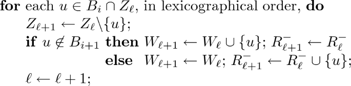
• Insertion steps:

  

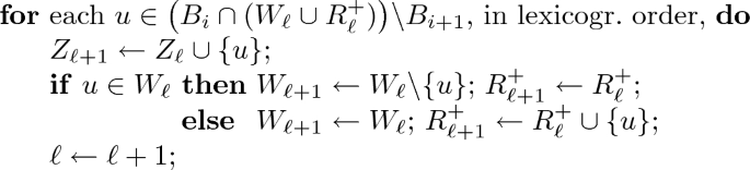
• Postprocessing: All elements of $R^-_{\ell +1}$ which do not belong to $B_{i+1}$ can now be safely added to $W_{\ell }$. This does not change the current independent set or add to the canonical path.

  $W_{\ell }\leftarrow W_{\ell } \cup (R_{\ell }^- {\setminus } B_{i+1})$; $R_{\ell }^-\leftarrow R_{\ell }^- \cap B_{i+1}$;

By construction, vertices added to $R_{\ell }^+$ are removed from $W_{\ell }$, so the “otherwise” case for insertion is precisely $u\in R_{\ell }^+$.

Observe that both $Z_\ell$ and $W_\ell$ are independent sets at every step. This is true initially (when $\ell =N$) and remains true. The preprocessing phases removes all vertices of $B_i\cap B_{i+1}$ from $W_\ell$, which makes room for other vertices to be inserted into the encoding later. A deletion step shrinks the current independent set and adds the removed vertex into $W_\ell$ or $R_\ell ^-$. A deleted vertex is only added to $R_\ell ^-$ if it belongs to $B_i\cap B_{i+1}$, and so might have a neighbour in $W_{\ell }$. In the insertion steps we add vertices from $\big (B_i\cap (W_\ell \cup R^+_{\ell })\big ){\setminus } B_{i+1}$ to $Z_\ell$, now that we have made room. Here $B_i$ is the last bag which contains the vertex being inserted into the independent set, so any neighbour of this vertex in X has already been deleted from the current independent set. This phase can only shrink the encoding $W_\ell$. Also observe that (16) holds for $(Z,W,R) = (Z_\ell ,W_\ell ,R_\ell )$ at every point. Finally, by construction we have $R_\ell \subseteq B_i$ at all times. Table 1 illustrates this construction for the graph in Fig. 1.

Table 1. The steps of the canonical path, processing each bag in order.

Each step of the canonical path alters the current independent set $Z_i$ by exactly one element of $X\oplus Y$. Every vertex of $X{\setminus } Y$ is removed from the current independent set at some point, and is never re-inserted, while every vertex of $Y{\setminus } X$ is inserted into the current independent set once, and is never removed. Vertices outside $X \oplus Y$ are never altered and belong to all or none of the independent sets in the canonical path. Therefore .

Lemma 3

At any transition $(Z,Z')$ which occurs during the processing of bag $B_i$, the set R of remembered vertices satisfies $R\subseteq B_i$, with $|R|\le p$ unless $Z\cap B_i = W\cap B_i = \varnothing$. In this case $R=B_i$, which gives $|R|=p+1$, and $Z' = Z\cup \{u\}$ for some $u\in B_i$.

Lemma 4

Given a transition $(Z,Z')$, the encoding W of Z and the set R of remembered vertices, we can uniquely reconstruct (X, Y) with $(Z,Z')\in \gamma _{XY}$.

Theorem 1

Let $G\in \mathcal {C}_p$ be a graph with n vertices and let $\lambda \ge 1/n$, where $p\ge 2$ is an integer. Then the Glauber dynamics with fugacity $\lambda$ on $\mathcal {I}(G)$ (and initial state $\varnothing$) has mixing time

$$ \tau _\varnothing (\varepsilon ) \le 2e\alpha (G)\, n^{p+1}\, \lambda ^p \Big (1+\max (\lambda ,1/\lambda )\Big )\Big (\alpha (G)\,\ln (n\lambda )+1+\ln (1/\varepsilon )\Big ).$$

When p is constant, this upper bound is polynomial in n and $\max (\lambda ,1/\lambda )$.

5 Recognisable Subclasses of $\mathcal {C}_p$

Theorem 1 shows that the Glauber dynamics for independent sets is rapidly mixing for any graph G in the class $\mathcal {C}_p$, where p is a fixed positive integer. However, the complexity of recognising membership in the class $\mathcal {C}_p$ is unknown. Therefore, we consider here three classes of graphs determined by small excluded subgraphs. These classes have polynomial time recognition algorithms. Note that we must always exclude large complete bipartite subgraphs. The three classes are nested. We will obtain better bounds for pathwidth in the smaller classes, and hence better mixing time bounds in Theorem 1.

5.1 Claw-Free Graphs

Claw-free graphs exclude the $K_{1,3}$, the claw. Claw-free graphs form an important superclass of line graphs [4], and independent sets in line graphs are matchings.

Lemma 5

Let G be a claw-free graph with independent sets $X, Y\in \mathcal {I}(G)$. Then $G[X\oplus Y]$ is a disjoint union of paths and cycles.

Lemma 6

Claw-free graphs are a proper subclass of $\mathcal {C}_2$.

5.2 Graphs with No Fork or Complete Bipartite Subgraph

Fork-free graphs exclude the following induced subgraph, the fork:

Two vertices u and v are false twins if $N(u)=N(v)$. In Fig. 2, vertices to which false twins can be added are indicated by red colour. Hence each graph containing a red vertex represents an infinite family of augmented graphs.

Fig. 2.

The path $P_9$, the cycle $C_8$, the augmented bipartite wheel $BW^*_3$, the cube $Q_3$, an augmented domino, followed by augmented paths $P_2^*$, $P_4^*$ and $P_5^*$. (Color figure online)

Lemma 7

A bipartite graph is fork-free if and only if every connected component is a path, a cycle of even length, a $BW^*_3$, a cube $Q_3$, or can be obtained from a complete bipartite graph by removing at most two edges that form a matching.

Lemma 8

For all integers $d \ge 1$ the fork-free graphs without induced $K_{d+1,d+1}$ have bipartite pathwidth at most $\max (4,d+2)$.

5.3 Graphs Free of Armchairs, Stirrers and Tripods

The graphs depicted below are called armchair, stirrer and tripod. A fast graph is a graph that contains none of these three as an induced subgraph.

Theorem 2

For every integer $d \ge 1$, a fast bipartite graph that does not contain $K_{d+1,d+1}$ as an induced subgraph has pathwidth at most $4d-1$.

6 Conclusions and Further Work

It is clearly NP-hard in general to determine the bipartite pathwidth of a graph, since it is NP-complete to determine the pathwidth of a bipartite graph. However, we need only determine whether ${\text {bpw}}(G)\le d$ for some constant d. The complexity of this question is less clear. Bodlaender [5] has shown that the question ${\text {pw}}(G)\le d$, can be answered in $O(2^{d^2}n)$ time. However, this implies nothing about ${\text {bpw}}(G)$.

In the case of claw-free graphs we can prove stronger sampling results using log-concavity. How far does log-concavity extends in this setting? Does it hold for fork-free graphs? Does some generalisation of log-concavity hold for graphs of bounded bipartite pathwidth? Where log-concavity holds, it allows us to approximate the number of independent sets of a given size. However, there is still the requirement of “amenability” [19]. Jerrum, Sinclair and Vigoda [20] have shown that this can be dispensed with in the case of matchings. Can this be done for claw-free graphs? More ambitiously, can the result of [20] be extended to fork-free graphs and larger classes of graphs of bounded bipartite pathwidth?

An extension would be to consider bipartite treewidth, ${\text {btw}}(G)$. Since ${\text {tw}}(G)= O({\text {pw}}(G)\log n)$ [6, Thm. 66], our results here immediately imply that bounded bipartite treewidth implies quasipolynomial mixing time for the Glauber dynamics. Can this be improved to polynomial time?

Finally, can approaches to approximate counting be employed for the independent set problem in particular graph classes? Patel and Regts [25] have used the Taylor expansion approach for claw-free graphs. Could this be extended?

References

Alekseev, V.E.: Polynomial algorithm for finding the largest independent sets in graphs without forks. Discrete Appl. Math. 135, 3–16 (2004)
Barvinok, A.: Computing the partition function of a polynomial on the Boolean cube. In: Loebl, M., Nešetřil, J., Thomas, R. (eds.) A Journey Through Discrete Mathematics, pp. 135–164. Springer, Cham (2017). https://doi.org/10.1007/978-3-319-44479-6_7
Bayati, M., Gamarnik, D., Katz, D., Nair, C., Tetali, P.: Simple deterministic approximation algorithms for counting matchings. In: Proceedings of the STOC, pp. 122–127 (2007)
Beineke, L.: Characterizations of derived graphs. J. Comb. Theory 9, 129–135 (1970)
Bodlaender, H.L.: A linear time algorithm for finding tree-decompositions of small treewidth. SIAM J. Comput. 25, 1305–1317 (1996)
Bodlander, H.L.: A partial \(k\)-arboretum of graphs with bounded treewidth. Theor. Comput. Sci. 209, 1–45 (1998)
Chudnovsky, M., Seymour, P.: The roots of the independence polynomial of a clawfree graph. J. Comb. Theory ( Ser. B) 97, 350–357 (2007)
Diaconis, P., Saloff-Coste, L.: Comparison theorems for reversible Markov chains. Ann. Appl. Probab. 3, 696–730 (1993)
Diaconis, P., Stroock, D.: Geometric bounds for eigenvalues of Markov chains. Ann. Appl. Probab. 1, 36–61 (1991)
Diestel, R.: Graph Theory. Graduate Texts in Mathematics, vol. 173. Springer, Heidelberg (2017). https://doi.org/10.1007/978-3-662-53622-3
Dyer, M., Goldberg, L.A., Greenhill, C., Jerrum, M.: On the relative complexity of approximate counting problems. Algorithmica 38, 471–500 (2003)
Dyer, M., Greenhill, C.: On Markov chains for independent sets. J. Algorithms 35, 17–49 (2000)
Dyer, M., Greenhill, C., Müller, H.: Counting independent sets in graphs with bounded bipartite pathwidth. Preprint: arXiv:1812.03195 (2018)
Efthymiou, C., Hayes, T., Stefankovic, D., Vigoda, E., Yin, Y.: Convergence of MCMC and loopy BP in the tree uniqueness region for the hard-core model. In: Proceedings of the FOCS 2016, pp. 704–713. IEEE (2016)
Greenhill, C.: The complexity of counting colourings and independent sets in sparse graphs and hypergraphs. Comput. Complex. 9, 52–72 (2000)
Harvey, N.J.A., Srivastava, P., Vondrák, J.: Computing the independence polynomial: from the tree threshold down to the roots. In: Proceedings of the SODA 2018, pp. 1557–1576 (2018)
Jerrum, M.: Mathematical foundations of the Markov chain Monte Carlo method. In: Habib, M., McDiarmid, C., Ramirez-Alfonsin, J., Reed, B. (eds.) Probabilistic Methods for Algorithmic Discrete Mathematics. AC, vol. 16, pp. 116–165. Springer, Heidelberg (1998). https://doi.org/10.1007/978-3-662-12788-9_4
Jerrum, M.: Counting, Sampling and Integrating: Algorithms and Complexity. Lectures in Mathematics - ETH Zürich. Birkhäuser, Basel (2003)
Jerrum, M., Sinclair, A.: Approximating the permanent. SIAM J. Comput. 18, 1149–1178 (1989)
Jerrum, M., Sinclair, A., Vigoda, E.: A polynomial-time approximation algorithm for the permanent of a matrix with non-negative entries. J. ACM 51, 671–697 (2004)
Jerrum, M.R., Valiant, L.G., Vazirani, V.V.: Random generation of combinatorial structures from a uniform distribution. Theoret. Comput. Sci. 43, 169–188 (1986)
Matthews, J.: Markov chains for sampling matchings, Ph.D. thesis, University of Edinburgh (2008)
Luby, M., Vigoda, E.: Approximately counting up to four. In: Proceedings of the STOC 1995, pp. 150–159. ACM (1995)
Minty, G.J.: On maximal independent sets of vertices in claw-free graphs. J. Comb. Theory Ser. B 28, 284–304 (1980)
Patel, V., Regts, G.: Deterministic polynomial-time approximation algorithms for partition functions and graph polynomials. SIAM J. Comput. 46, 1893–1919 (2017)
Provan, J.S., Ball, M.O.: The complexity of counting cuts and of computing the probability that a graph is connected. SIAM J. Comput. 12, 777–788 (1983)
Robertson, N., Seymour, P.D.: Graph minors I: excluding a forest. J. Comb. Theory Ser. B 35, 39–61 (1983)
Sinclair, A.: Improved bounds for mixing rates of Markov chains and multicommodity flow. Comb. Probab. Comput. 1, 351–370 (1992)
Sly, A.: Computational transition at the uniqueness threshold. In: Proceedings of the FOCS 2010, pp. 287–296. IEEE (2010)
Vadhan, S.P.: The complexity of counting in sparse, regular, and planar graphs. SIAM J. Comput. 31, 398–427 (2001)
Weitz, D.: Counting independent sets up to the tree threshold. In: Proceedings of the STOC 2006, pp. 140–149. ACM (2006)
Author information
Authors and Affiliations
Corresponding author
Editor information
Editors and Affiliations
Rights and permissions
Copyright information
© 2019 Springer Nature Switzerland AG
About this paper
Cite this paper
Dyer, M., Greenhill, C., Müller, H. (2019). Counting Independent Sets in Graphs with Bounded Bipartite Pathwidth. In: Sau, I., Thilikos, D. (eds) Graph-Theoretic Concepts in Computer Science. WG 2019. Lecture Notes in Computer Science(), vol 11789. Springer, Cham. https://doi.org/10.1007/978-3-030-30786-8_23
Download citation
DOI: https://doi.org/10.1007/978-3-030-30786-8_23
Published:
Publisher Name: Springer, Cham
Print ISBN: 978-3-030-30785-1
Online ISBN: 978-3-030-30786-8
eBook Packages: Computer ScienceComputer Science (R0)