On the Acceleration of Forward-Backward Splitting via an Inexact Newton Method

Abstract

We propose a Forward-Backward Truncated-Newton method (FBTN) for minimizing the sum of two convex functions, one of which smooth. Unlike other proximal Newton methods, our approach does not involve the employment of variable metrics, but is rather based on a reformulation of the original problem as the unconstrained minimization of a continuously differentiable function, the forward-backward envelope (FBE). We introduce a generalized Hessian for the FBE that symmetrizes the generalized Jacobian of the nonlinear system of equations representing the optimality conditions for the problem. This enables the employment of conjugate gradient method (CG) for efficiently solving the resulting (regularized) linear systems, which can be done inexactly. The employment of CG prevents the computation of full (generalized) Jacobians, as it requires only (generalized) directional derivatives. The resulting algorithm is globally (subsequentially) convergent, Q-linearly under an error bound condition, and up to Q-superlinearly and Q-quadratically under regularity assumptions at the possibly non-isolated limit point.

15.1 Introduction

In this work we focus on convex composite optimization problems of the form

$$\displaystyle \begin{aligned} \operatorname{minimize}_{x\in\mathbb{R}^n}\varphi(x)\equiv f(x)+g(x), \end{aligned} $$

(15.1)

where $f:\mathbb {R}^n\rightarrow \mathbb {R}$ is convex, twice continuously differentiable and with L _f-Lipschitz-continuous gradient, and $g:\mathbb {R}^n\rightarrow \mathbb {R}\cup \{\infty \}$ has a cheaply computable proximal mapping [51]. To ease the notation, throughout the chapter we indicate

(15.2)

Problems of the form (15.1) are abundant in many scientific areas such as control, signal processing, system identification, machine learning, and image analysis, to name a few. For example, when g is the indicator of a convex set then (15.1) becomes a constrained optimization problem, while for $f(x)=\frac 12\|Ax-b\|{ }^2$ and g(x) = λ∥x∥₁ it becomes the ℓ ₁-regularized least-squares problem (lasso) which is the main building block of compressed sensing. When g is equal to the nuclear norm, then (15.1) models low-rank matrix recovery problems. Finally, conic optimization problems such as linear, second-order cone, and semidefinite programs can be brought into the form of (15.1), see [31].

Perhaps the most well-known algorithm for problems in the form (15.1) is the forward-backward splitting (FBS) or proximal gradient method [16, 40], that interleaves gradient descent steps on the smooth function and proximal steps on the nonsmooth one, see Section 15.3.1. Accelerated versions of FBS, based on the work of Nesterov [5, 54, 77], have also gained popularity. Although these algorithms share favorable global convergence rate estimates of order O(ε ⁻¹) or O(ε ^−1∕2) (where ε is the solution accuracy), they are first-order methods and therefore usually effective at computing solutions of low or medium accuracy only. An evident remedy is to include second-order information by replacing the Euclidean norm in the proximal mapping with that induced by the Hessian of f at x or some approximation of it, mimicking Newton or quasi-Newton methods for unconstrained problems [6, 32, 42]. However, a severe limitation of the approach is that, unless Q has a special structure, the computation of the proximal mapping becomes very hard. For example, if φ models a lasso problem, the corresponding subproblem is as hard as the original problem.

In this work we follow a different approach by reformulating the nonsmooth constrained problem (15.1) into the smooth unconstrained minimization of the forward-backward envelope (FBE) [57], a real-valued, continuously differentiable, exact penalty function for φ. Although the FBE might fail to be twice continuously differentiable, by using tools from nonsmooth analysis we show that one can design Newton-like methods to address its minimization, that achieve Q-superlinear asymptotic rates of convergence under nondegeneracy and (generalized) smoothness conditions on the set of solutions. Furthermore, by suitably interleaving FBS and Newton-like iterations the proposed algorithm also enjoys good complexity guarantees provided by a global (non-asymptotic) convergence rate. Unlike the approaches of [6, 32], where the corresponding subproblems are expensive to solve, our algorithm only requires the inexact solution of a linear system to compute the Newton-type direction, which can be done efficiently with a memory-free CG method.

Our approach combines and extends ideas stemming from the literature on merit functions for variational inequalities (VIs) and complementarity problems (CPs), specifically the reformulation of a VI as a constrained continuously differentiable optimization problem via the regularized gap function [23] and as an unconstrained continuously differentiable optimization problem via the D-gap function [79] (see [19, §10] for a survey and [38, 58] for applications to constrained optimization and model predictive control of dynamical systems).

15.1.1 Contributions

We propose an algorithm that addresses problem (15.1) by means of a Newton-like method on the FBE. Differently from a direct application of the classical Newton method, our approach does not require twice differentiability of the FBE (which would impose additional properties on f and g), but merely twice differentiability of f. This is possible thanks to the introduction of an approximate generalized Hessian which only requires access to ∇² f and to the generalized (Clarke) Jacobian of the proximal mapping of g, as opposed to third-order derivatives and classical Jacobian, respectively. Moreover, it allows for inexact solutions of linear systems to compute the update direction, which can be done efficiently with a truncated CG method; in particular, no computation of full (generalized) Hessian matrices is necessary, as only (generalized) directional derivatives are needed. The method is thus particularly appealing when the Clarke Jacobians are sparse and/or well structured, so that the implementation of CG becomes extremely efficient. Under an error bound condition and a (semi)smoothness assumption at the limit point, which is not required to be isolated, the algorithm exhibits asymptotic Q-superlinear rates. For the reader’s convenience we collect explicit formulas of the needed Jacobians of the proximal mapping for a wide range of frequently encountered functions, and discuss when they satisfy the needed semismoothness requirements that enable superlinear rates.

15.1.2 Related Work

This work is a revised version of the unpublished manuscript [59] and extends ideas proposed in [57], where the FBE is first introduced. Other FBE-based algorithms are proposed in [69, 71, 75]; differently from the truncated-CG type of approximation proposed here, they all employ quasi-Newton directions to mimic second-order information. The underlying ideas can also be extended to enhance other popular proximal splitting algorithms: the Douglas Rachford splitting (DRS) and the alternating direction method of multipliers (ADMM) [74], and for strongly convex problems also the alternating minimization algorithm (AMA) [70].

The algorithm proposed in this chapter adopts the recent techniques investigated in [71, 75] to enhance and greatly simplify the scheme in [59]. In particular, Q-linear and Q-superlinear rates of convergence are established under an error bound condition, as opposed to uniqueness of the solution. The proofs of superlinear convergence with an error bound pattern the arguments in [82, 83], although with less conservative requirements.

15.1.3 Organization

The work is structured as follows. In Section 15.2 we introduce the adopted notation and list some known facts on generalized differentiability needed in the sequel. Section 15.3 offers an overview on the connections between FBS and the proximal point algorithm, and serves as a prelude to Section 15.4 where the forward-backward envelope function is introduced and analyzed. Section 15.5 deals with the proposed truncated-Newton algorithm and its convergence analysis. In Section 15.6 we collect explicit formulas for the generalized Jacobian of the proximal mapping of a rich list of nonsmooth functions, needed for computing the update directions in the proposed algorithm. Finally, Section 15.7 draws some conclusions.

15.2 Preliminaries

15.2.1 Notation and Known Facts

Our notation is standard and follows that of convex analysis textbooks [2, 8, 28, 63]. For the sake of clarity we now properly specify the adopted conventions, and briefly recap known definitions and facts in convex analysis. The interested reader is referred to the above-mentioned textbooks for the details.

Matrices and Vectors

The n × n identity matrix is denoted as I_n, and the $\mathbb {R}^n$ vector with all elements equal to 1 is as 1 _n; whenever n is clear from context we simply write I or 1, respectively. We use the Kronecker symbol δ _i,j for the (i, j)-th entry of I. Given $v\in \mathbb {R}^n$, with $\operatorname {diag} v$ we indicate the n × n diagonal matrix whose i-th diagonal entry is v _i. With $\operatorname {S}(\mathbb {R}^n)$, $\operatorname {S}_+(\mathbb {R}^n)$, and $\operatorname {S}_{++}(\mathbb {R}^n)$ we denote respectively the set of symmetric, symmetric positive semidefinite, and symmetric positive definite matrices in $\mathbb {R}^{n\times n}$.

The minimum and maximum eigenvalues of $H\in \operatorname {S}(\mathbb {R}^n)$ are denoted as λ _min(H) and λ _max(H), respectively. For $Q,R\in \operatorname {S}(R^n)$ we write Q ≽ R to indicate that $Q-R\in \operatorname {S}_+(\mathbb {R}^n)$, and similarly Q ≻ R indicates that $Q-R\in \operatorname {S}_{++}(\mathbb {R}^n)$. Any matrix $Q\in \operatorname {S}_+(\mathbb {R}^n)$ induces the semi-norm ∥⋅∥_Q on $\mathbb {R}^n$, where $\|x\|{ }_Q^2\mathrel{\mathop:}= \langle {}x{},{}Qx{}\rangle$; in case Q = I, that is, for the Euclidean norm, we omit the subscript and simply write ∥⋅∥. No ambiguity occurs in adopting the same notation for the induced matrix norm, namely $\|M\|\mathrel{\mathop:}= \max \{{\|Mx\|} \vert x\in \mathbb {R}^n,~\|x\|=1\vert \}$ for $M\in \mathbb {R}^{n\times n}$.

Topology

The convex hull of a set $E\subseteq \mathbb {R}^n$, denoted as $\operatorname {conv} E$, is the smallest convex set that contains E (the intersection of convex sets is still convex). The affine hull $\operatorname {aff} E$ and the conic hull $\operatorname {cone} E$ are defined accordingly. Specifically,

The closure and interior of E are denoted as $\operatorname *{\mathrm {cl}} E$ and $\operatorname {int} E$, respectively, whereas its relative interior, namely the interior of E as a subspace of $\operatorname {aff} E$, is denoted as $\operatorname {relint} E$. With and we indicate, respectively, the open and closed balls centered at x with radius r.

Sequences

The notation represents a sequence indexed by elements of the set K, and given a set E we write to indicate that a ^k ∈ E for all indices k ∈ K. We say that is summable if ∑_{k ∈ K}∥a ^k∥ is finite, and square-summable if is summable. We say that the sequence converges to a point $a\in \mathbb {R}^n$ superlinearly if either a ^k = a for some $k\in {\mathbb N}$, or ∥a ^k+1 − a∥∕∥a ^k − a∥→ 0; if ∥a ^k+1 − a∥∕∥a ^k − a∥^q is bounded for some q > 1, then we say that the sequence converges superlinearly with order q, and in case q = 2 we say that the convergence is quadratic.

Extended-Real Valued Functions

The extended-real line is . Given a function $h:\mathbb {R}^n\rightarrow [-\infty ,\infty ]$, its epigraph is the set

while its domain is

and for $\alpha \in \mathbb {R}$ its α-level set is

Function h is said to be lower semicontinuous (lsc) if $\operatorname *{\mathrm {epi}} h$ is a closed set in $\mathbb {R}^{n+1}$ (equivalently, h is said to be closed); in particular, all level sets of an lsc function are closed. We say that h is proper if h > −∞ and $\operatorname {{\mathrm {dom}}} h\neq \emptyset$, and that it is level bounded if for all $\alpha \in \mathbb {R}$ the level set $\operatorname {lev}_{\leq \alpha }h$ is a bounded subset of $\mathbb {R}^n$.

Continuity and Smoothness

A function $G:\mathbb {R}^n\rightarrow \mathbb {R}^m$ is 𝜗-Hölder continuous for some 𝜗 > 0 if there exists L ≥ 0 such that

$$\displaystyle \begin{aligned} \|G(x)-G(x')\| {}\leq{} L\|x-x'\|{}^\vartheta \end{aligned} $$

(15.3)

for all x, x′. In case 𝜗 = 1 we say that G is (L-)Lipschitz continuous. G is strictly differentiable at $\bar x\in \mathbb {R}^n$ if the Jacobian matrix $JG(\bar x) {}\mathrel{\mathop:}= {} \big (\frac {\partial G_i}{\partial x_j}(\bar x)\big )_{i,j}$ exists and

(15.4)

The class of functions $h:\mathbb {R}^n\rightarrow \mathbb {R}$ that are k times continuously differentiable is denoted as $C^k(\mathbb {R}^n)$. We write $h\in C^{1,1}(\mathbb {R}^n)$ to indicate that $h\in C^1(\mathbb {R}^n)$ and that ∇h is Lipschitz continuous with modulus L _h. To simplify the terminology, we will say that such an h is L _h -smooth. If h is L _h-smooth and convex, then for any $u,v\in \mathbb {R}^n$

(15.5)

Moreover, having $h\in C^{1,1}(\mathbb {R}^n)$ and μ _h-strongly convex is equivalent to having

$$\displaystyle \begin{aligned} \mu_h\|v-u\|{}^2 {}\leq{} \langle{}\nabla h(v)-\nabla h(u){},{}v-u{}\rangle {}\leq{} L_h\|v-u\|{}^2 \end{aligned} $$

(15.6)

for all $u,v\in \mathbb {R}^n$.

Set-Valued Mappings

We use the notation $H:\mathbb {R}^n\rightrightarrows \mathbb {R}^m$ to indicate a point-to-set function $H:\mathbb {R}^n\rightarrow \mathcal P(\mathbb {R}^m)$, where $\mathcal P(\mathbb {R}^m)$ is the power set of $\mathbb {R}^m$ (the set of all subsets of $\mathbb {R}^m$). The graph of H is the set

while its domain is

We say that H is outer semicontinuous (osc) at $\bar x\in \operatorname {{\mathrm {dom}}} H$ if for any ε > 0 there exists δ > 0 such that for all . In particular, this implies that whenever converges to x and converges to y with y ^k ∈ H(x ^k) for all k, it holds that y ∈ H(x). We say that H is osc (without mention of a point) if H is osc at every point of its domain or, equivalently, if $\operatorname {gph} H$ is a closed subset of $\mathbb {R}^n\times \mathbb {R}^m$ (notice that this notion does not reduce to lower semicontinuity for a single-valued function H).

Convex Analysis

The indicator function of a set $S\subseteq \mathbb {R}^n$ is denoted as $\operatorname {\delta }_S:\mathbb {R}^n\rightarrow \overline {\mathbb {R}}$, namely

(15.7)

If S is nonempty closed and convex, then $\operatorname {\delta }_S$ is proper convex and lsc, and both the projection $\operatorname {\mathscr P}_S:\mathbb {R}^n\rightarrow \mathbb {R}^n$ and the distance $\operatorname {dist}({}\cdot {},S):\mathbb {R}^n\rightarrow [0,\infty )$ are well-defined functions, given by $\operatorname {\mathscr P}_S(x)= \operatorname *{\mathrm {argmin}} \nolimits _{z\in S}\|z-x\|$ and $\operatorname {dist}(x,S)=\min _{z\in S}\|z-x\|$, respectively.

The subdifferential of h is the set-valued mapping $\partial h:\mathbb {R}^n\rightrightarrows \mathbb {R}^n$ defined as

(15.8)

A vector v ∈ ∂h(x) is called a subgradient of h at x. It holds that $\operatorname {{\mathrm {dom}}}\partial h\subseteq \operatorname {{\mathrm {dom}}} h$, and if h is proper and convex, then $\operatorname {{\mathrm {dom}}}\partial h$ is a nonempty convex set containing $\operatorname {relint} \operatorname {{\mathrm {dom}}} h$, and ∂h(x) is convex and closed for all $x\in \mathbb {R}^n$.

A function h is said to be μ-strongly convex for some μ ≥ 0 if $h-\tfrac \mu 2\|{}\cdot {}\|{ }^2$ is convex. Unless differently specified, we allow for μ = 0 which corresponds to h being convex but not strongly so. If μ > 0, then h has a unique (global) minimizer.

15.2.2 Generalized Differentiability

Due to its inherent nonsmooth nature, classical notions of differentiability may not be directly applicable in problem (15.1). This subsection contains some definitions and known facts on generalized differentiability that will be needed later on in the chapter. The interested reader is referred to the textbooks [15, 19, 65] for the details.

Definition 15.2.1 (Bouligand and Clarke Subdifferentials)

Let $G:\mathbb {R}^n\rightarrow \mathbb {R}^m$ be locally Lipschitz continuous, and let $C_G\subseteq \mathbb {R}^n$ be the set of points at which G is differentiable (in particular has measure zero). The B-subdifferential (also known as Bouligand or limiting Jacobian) of G at $\bar x$ is the set-valued mapping $\partial _BG:\mathbb {R}^n\rightrightarrows \mathbb {R}^{m\times n}$ defined as

(15.9)

whereas the (Clarke) generalized Jacobian of G at $\bar x$ is $\partial _CG:\mathbb {R}^n\rightrightarrows \mathbb {R}^{m\times n}$ given by

$$\displaystyle \begin{aligned} \partial_CG(\bar x)\mathrel{\mathop:}=\operatorname{conv}(\partial_BG(\bar x)).\end{aligned} $$

(15.10)

If $G:\mathbb {R}^n\rightarrow \mathbb {R}^m$ is locally Lipschitz on $\mathbb {R}^n$, then ∂ _C G(x) is a nonempty, convex, and compact subset of $\mathbb {R}^{m\times n}$ matrices, and as a set-valued mapping it is osc at every $x\in \mathbb {R}^n$. Semismooth functions [60] are precisely Lipschitz-continuous mappings for which the generalized Jacobian (and consequently the B-subdifferential) furnishes a first-order approximation.

Definition 15.2.2 (Semismooth Mappings)

Let $G:\mathbb {R}^n\rightarrow \mathbb {R}^m$ be locally Lipschitz continuous at $\bar x$. We say that G is semismooth at $\bar x$ if

(15.11a)

We say that G is 𝜗-order semismooth for some 𝜗 > 0 if the condition can be strengthened to

(15.11b)

and in case 𝜗 = 1 we say that G is strongly semismooth.

To simplify the notation, we adopt the small-o and big-O convention to write expressions as (15.11a) in the compact form $G(x)+H(\bar x-x)-G(\bar x) {}={} o(\|x-\bar x\|)$, and similarly (15.11b) as $G(x)+H(\bar x-x)-G(\bar x) {}={} O(\|x-\bar x\|{ }^{1+\vartheta })$. We remark that the original definition of semismoothness given by [49] requires G to be directionally differentiable at x. The definition given here is the one employed by [25]. It is also worth remarking that ∂ _C G(x) can be replaced with the smaller set ∂ _B G(x) in Definition 15.2.2. Fortunately, the class of semismooth mappings is rich enough to include many functions arising in interesting applications. For example, piecewise smooth (PC ¹ ) mappings are semismooth everywhere. Recall that a continuous mapping $G:\mathbb {R}^n\rightarrow \mathbb {R}^m$ is PC ¹ if there exists a finite collection of smooth mappings $G_i:\mathbb {R}^n\rightarrow \mathbb {R}^m$, i = 1, …, N, such that

(15.12)

The definition of PC ¹ mapping given here is less general than the one of, e.g., [66, §4] but it suffices for our purposes. For every $x\in \mathbb {R}^n$ we introduce the set of essentially active indices

(15.13)

In other words, $I_G^e(x)$ contains only indices of the pieces G _i for which there exists a full-dimensional set on which G agrees with G _i. In accordance with Definition 15.2.1, the generalized Jacobian of G at x is the convex hull of the Jacobians of the essentially active pieces, i.e., [66, Prop. 4.3.1]

(15.14)

The following definition is taken from [19, Def. 7.5.13].

Definition 15.2.3 (Linear Newton Approximation)

Let $G:\mathbb {R}^n\rightarrow \mathbb {R}^m$ be continuous on $\mathbb {R}^n$. We say that G admits a linear Newton approximation (LNA) at $\bar x\in \mathbb {R}^n$ if there exists a set-valued mapping $\mathcal H:\mathbb {R}^n\rightrightarrows \mathbb {R}^{m\times n}$ that has nonempty compact images, is outer semicontinuous at $\bar x$, and

If for some 𝜗 > 0 the condition can be strengthened to

then we say that $\mathcal H$ is a 𝜗-order LNA, and if 𝜗 = 1 we say that $\mathcal H$ is a strong LNA.

Functions G as in Definition 15.2.3 are also referred to as $\mathcal H$-semismooth in the literature, see, e.g., [78], however we prefer to stick to the terminology of [19] and rather say that $\mathcal H$ is a LNA for G. Arguably the most notable example of a LNA for semismooth mappings is the generalized Jacobian, cf. Definition 15.2.1. However, semismooth mappings can admit LNAs different from the generalized Jacobian. More importantly, mappings that are not semismooth may also admit a LNA.

Lemma 15.2.4 ([19, Prop. 7.4.10])

Let $h\in C^1(\mathbb {R}^n)$ and suppose that $\mathcal H:\mathbb {R}^n\rightrightarrows \mathbb {R}^{n\times n}$ is a LNA for ∇h at $\bar x$ . Then,

(15.15)

We remark that although [19, Prop. 7.4.10] assumes semismoothness of ∇h at $\bar x$ and uses ∂ _C(∇h) in place of $\mathcal H$; however, exactly the same arguments apply for any LNA of ∇h at $\bar x$ even without the semismoothness assumption.

15.3 Proximal Algorithms

15.3.1 Proximal Point and Moreau Envelope

The proximal mapping of a proper closed and convex function $h:\mathbb {R}^n\rightarrow \overline {\mathbb {R}}$ with parameter γ > 0 is $\operatorname {prox}_{\gamma h}:\mathbb {R}^n\rightarrow \mathbb {R}^n$, given by

(15.16)

The majorization model $\mathcal M_\gamma ^h(x;{}\cdot {})$ is a proper and strongly convex function, and therefore has a unique minimizer. The value function, as opposed to the minimizer, defines the Moreau envelope $h^\gamma :\mathbb {R}^n\rightarrow \mathbb {R}$, namely

(15.17)

which is real valued and Lipschitz differentiable, despite the fact that h might be extended-real valued. Properties of the Moreau envelope and the proximal mapping are well documented in the literature, see, e.g., [2, §24]. For example, $\operatorname {prox}_{\gamma h}$ is nonexpansive (Lipschitz continuous with modulus 1) and is characterized by the implicit inclusion

$$\displaystyle \begin{aligned} \hat x=\operatorname{prox}_{\gamma h}(x) \quad \Leftrightarrow\quad \frac{1}{\gamma}(x-\hat x)\in\partial h(\hat x). \end{aligned} $$

(15.18)

For the sake of a brief recap, we now list some other important known properties. Theorem 15.3.1 provides some relations between h and its Moreau envelope h ^γ, which we informally refer to as sandwich property for apparent reasons, cf. Figure 15.1. Theorem 15.3.2 highlights that the minimization of a (proper, lsc and) convex function can be expressed as the convex smooth minimization of its Moreau envelope.

Fig. 15.1

Moreau envelope of the function $\varphi (x) = \tfrac 13x^3+x^2-x+1+\operatorname {\delta }_{[0,\infty )}(x)$ with parameter γ = 0.2. At each point x, the Moreau envelope φ ^γ is the minimum of the quadratic majorization model $\mathcal M_\gamma ^\varphi =\varphi + \frac {1}{2\gamma }({}\cdot {}-x)^2$, the unique minimizer being, by definition, the proximal point $\hat x\mathrel{\mathop:}= \operatorname {prox}_{\gamma \varphi }(x)$. It is a convex smooth lower bound to φ, despite the fact that φ might be extended-real valued. Function φ and its Moreau envelope φ ^γ have same $\inf$ and $\operatorname *{\mathrm {argmin}}$; in fact, the two functions agree (only) on the set of minimizers. In general, φ ^γ is sandwiched as $\varphi \circ \operatorname {prox}_{\gamma \varphi }\leq \varphi ^\gamma \leq \varphi$

Theorem 15.3.1 (Moreau Envelope: Sandwich Property [2, 12])

For all γ > 0 the following hold for the cost function φ:

• (i) for all $x\in \mathbb {R}^n$ where $\hat x\mathrel{\mathop:}= \operatorname {prox}_{\gamma \varphi }(x)$ ;

• (ii) for all $x\in \mathbb {R}^n$ where $\hat x\mathrel{\mathop:}= \operatorname {prox}_{\gamma \varphi }(x)$ ;

• (iii) iff $x\in \operatorname *{\mathrm {argmin}}\varphi$.

Proof

• • 15.3.1(i) . This fact is shown in [12, Lem. 3.2] for a more general notion of proximal point operator; namely, the square Euclidean norm appearing in (15.16) and (15.17) can be replaced by arbitrary Bregman divergences. In this simpler case, since $\tfrac 1\gamma (x-\hat x)$ is a subgradient of φ at $\hat x$, cf. (15.18), we have

  

  (15.19)

  The claim now follows by subtracting $\tfrac {1}{2\gamma }\|x-\hat x\|{ }^2$ from both sides.

• • 15.3.1(ii) . Follows by definition, cf. (15.16) and (15.17).

• • 15.3.1(iii) . See [2, Prop. 17.5]. □

□

Theorem 15.3.2 (Moreau Envelope: Convex Smooth Minimization Equivalence [2])

For all γ > 0 the following hold for the cost function φ:

• (i) φ ^γ is convex and smooth with $L_{\varphi ^\gamma }=\gamma ^{-1}$ and $\nabla \varphi ^\gamma (x) {}={} \gamma ^{-1}\big (x-\operatorname {prox}_{\gamma \varphi }(x)\big )$ ;

• (ii) $\inf \varphi =\inf \varphi ^\gamma$ ;

• (iii) $x_\star \in \operatorname *{\mathrm {argmin}}\varphi$ iff $x_\star \in \operatorname *{\mathrm {argmin}}\varphi ^\gamma$ iff ∇φ ^γ(x _⋆) = 0.

Proof

• • 15.3.2(i) . See [2, Prop.s 12.15 and 12.30].

• • 15.3.2(ii) . See [2, Prop. 12.9(iii)].

• • 15.3.2(iii) . See [2, Prop. 17.5]. □

□

As a consequence of Theorem 15.3.2, one can address the minimization of the convex but possibly nonsmooth and extended-real-valued function φ by means of gradient descent on the smooth envelope function φ ^γ with stepsize $0<\tau <{2}/{L_{\varphi _\gamma }}=2\gamma$. As first noticed by Rockafellar [64], this simply amounts to (relaxed) fixed-point iterations of the proximal point operator, namely

$$\displaystyle \begin{aligned} x^+=(1-\lambda)x+\lambda\operatorname{prox}_{\gamma\varphi}(x), \end{aligned} $$

(15.20)

where λ = τ∕γ ∈ (0, 2) is a possible relaxation parameter. The scheme, known as proximal point algorithm (PPA) and first introduced by Martinet [45], is well covered by the broad theory of monotone operators, where convergence properties can be easily derived with simple tools of Fejérian monotonicity, see, e.g., [2, Thm.s 23.41 and 27.1]. Nevertheless, not only does the interpretation as gradient method provide a beautiful theoretical link, but it also enables the employment of acceleration techniques exclusively stemming from smooth unconstrained optimization, such as Nesterov’s extrapolation [26] or quasi-Newton schemes [13], see also [7] for extensions to the dual formulation.

15.3.2 Forward-Backward Splitting

While it is true that every convex minimization problem can be smoothened by means of the Moreau envelope, unfortunately it is often the case that the computation of the proximal operator (which is needed to evaluate the envelope) is as hard as solving the original problem. For instance, evaluating the Moreau envelope of the cost of modeling a convex QP at one point amounts to solving another QP with same constraints and augmented cost. To overcome this limitation there comes the idea of splitting schemes, which decompose a complex problem in small components which are easier to operate onto. A popular such scheme is the forward-backward splitting (FBS), which addresses minimization problems of the form (15.1).

Given a point $x\in \mathbb {R}^n$, one iteration of forward-backward splitting (FBS) for problem (15.1) with stepsize γ > 0 and relaxation λ > 0 consists in

(15.21)

where

(15.22)

is the forward-backward operator, characterized as

(15.23)

as it follows from (15.18). FBS interleaves a gradient descent step on f and a proximal point step on g, and as such it is also known as proximal gradient method. If both f and g are (lsc, proper and) convex, then the solutions to (15.1) are exactly the fixed points of the forward-backward operator T _γ. In other words,

(15.24)

where

(15.25)

is the forward-backward residual.¹ FBS iterations (15.21) are well known to converge to a solution to (15.1) provided that f is smooth and that the parameters are chosen as γ ∈ (0, 2∕L _f) and λ ∈ (0, 2 − γL _f∕2) [2, Cor. 28.9] (λ = 1, which is always feasible, is the typical choice).

15.3.3 Error Bounds and Quadratic Growth

We conclude the section with some inequalities that will be useful in the sequel.

Lemma 15.3.3

Suppose that $\mathcal X_\star$ is nonempty. Then,

$$\displaystyle \begin{aligned} \varphi(x)-\varphi_\star {}\leq{} \operatorname{dist}(0,\partial\varphi(x)) \operatorname{dist}(x,\mathcal X_\star) \quad \forall x\in\mathbb{R}^n. \end{aligned} $$

(15.26)

Proof

From the subgradient inequality it follows that for all $x_\star \in \mathcal X_\star$ and v ∈ ∂φ(x) we have

$$\displaystyle \begin{aligned} \varphi(x)-\varphi_\star {}={} \varphi(x)-\varphi(x_\star) {}\leq{} \langle{}v{},{}x-x_{\star{}}\rangle {}\leq{} \|v\|\|x-x_\star\|\end{aligned} $$

(15.27)

and the claimed inequality follows from the arbitrarity of x _⋆ and v. □

Lemma 15.3.4

Suppose that $\mathcal X_\star$ is nonempty. For all $x\in \mathbb {R}^n$ and γ > 0 the following holds:

(15.28)

Proof

Let . The characterization (15.23) of implies that

(15.29)

After trivial rearrangements the sought inequality follows. □

Further interesting inequalities can be derived if the cost function φ satisfies an error bound, which can be regarded as a generalization of strong convexity that does not require uniqueness of the minimizer. The interested reader is referred to [3, 17, 43, 55] and the references therein for extensive discussions.

Definition 15.3.5 (Quadratic Growth and Error Bound)

Suppose that $\mathcal X_\star \neq \emptyset$. Given μ, ν > 0, we say that

• 1. φ satisfies the quadratic growth with constants (μ, ν) if

  

  (15.30)

• 2. φ satisfies the error bound with constants (μ, ν) if

  

  (15.31)

In case ν = ∞ we say that the properties are satisfied globally.

Theorem 15.3.6 ([17, Thm. 3.3])

For a proper convex and lsc function, the quadratic growth with constants (μ, ν) is equivalent to the error bound with same constants.

Lemma 15.3.7 (Globality of Quadratic Growth)

Suppose that φ satisfies the quadratic growth with constants (μ, ν). Then, for every ν′ > ν it satisfies the quadratic growth with constants (μ′, ν′), where

(15.32)

Proof

Let ν′ > ν be fixed, and let $x\in \operatorname {lev}_{\leq \varphi _\star +\nu '}$ be arbitrary. Since μ′≤ μ, the claim is trivial if φ(x) ≤ φ _⋆ + ν; we may thus suppose that φ(x) > φ _⋆ + ν. Let z be the projection of x onto the (nonempty closed and convex) level set $\operatorname {lev}_{\leq \varphi _\star +\nu }$, and observe that φ(z) = φ _⋆ + ν. With Lemma 15.3.3 and Theorem 15.3.6 we can upper bound ν as

(15.33)

Moreover, it follows from [28, Thm. 1.3.5] that there exists a subgradient v ∈ ∂φ(z) such that 〈v, x − z〉 = ∥v∥∥x − z∥. Then,

(15.34)

By subtracting φ(z) from the first and last terms we obtain

(15.35)

which implies

(15.36)

Thus,

using the quadratic growth at z and the inequality (15.36)

By using the fact that $a^2+b^2\geq \frac 12(a+b)^2$ for any $a,b\in \mathbb {R}$ together with the triangular inequality $\operatorname {dist}(x,\mathcal X_\star )\leq \|x-z\|+\operatorname {dist}(z,\mathcal X_\star )$, we conclude that $\varphi (x) {}-{} \varphi _\star {}\geq {} \tfrac {\mu '}{2} \operatorname {dist}(x,\mathcal X_\star )^2$, with μ′ as in the statement. Since μ′ depends only on μ, ν, and ν′, from the arbitrarity of $x\in \operatorname {lev}_{\leq \varphi _\star +\nu '}$ the claim follows. □

Theorem 15.3.8 ([17, Cor. 3.6])

Suppose that φ satisfies the quadratic growth with constants (μ, ν). Then, for all γ ∈ (0, 1∕L _f) and $x\in \operatorname {lev}_{\leq \varphi _\star +\nu }\varphi$ we have

(15.37)

15.4 Forward-Backward Envelope

There are clearly infinite ways of representing the (proper, lsc and) convex function φ in (15.1) as the sum of two convex functions f and g with f smooth, and each of these choices leads to a different FBS operator T _γ. If f = 0, for instance, then T _γ reduces to $\operatorname {prox}_{\gamma \varphi }$, and consequently FBS (15.21) to the PPA (15.20). A natural question then arises, whether a function exists that serves as “envelope” for FBS in the same way that φ _γ does for $\operatorname {prox}_{\gamma \varphi }$. We will now provide a positive answer to this question by reformulating the nonsmooth problem (15.1) as the minimization of a differentiable function. To this end, the following requirements on f and g will be assumed throughout the chapter without further mention.

Assumption I (Basic Requirements) In problem (15.1),

• (i) $f:\mathbb {R}^n\rightarrow \mathbb {R}$ is convex, twice continuously differentiable and L _f -smooth;

• (ii) is lsc, proper, and convex.

Compared to the classical FBS assumptions, the only additional requirement is twice differentiability of f. This ensures that the forward operator is differentiable; we denote its Jacobian as $Q_\gamma :\mathbb {R}^n\rightarrow \mathbb {R}^{n\times n}$, namely

(15.38)

Notice that, due to the bound (which follows from L _f-smoothness of f, see [53, Lem. 1.2.2]) Q _γ(x) is invertible (in fact, positive definite) whenever γ < 1∕L _f. Moreover, due to the chain rule and Theorem 15.3.2(i) we have that

Rearranging,

we obtain the gradient of a real-valued function, which we define as follows.

Definition 15.4.1 (Forward-Backward Envelope) The forward-backward envelope (FBE) for the composite minimization problem (15.1) is the function $\varphi _\gamma :\mathbb {R}^n\rightarrow \mathbb {R}$ defined as

(15.39)

In the next section we discuss some of the favorable properties enjoyed by the FBE.

15.4.1 Basic Properties

We already verified that the FBE is differentiable with gradient

(15.40)

In particular, for γ < 1∕L _f one obtains that a FBS step is a (scaled) gradient descent step on the FBE, similarly as the relation between Moreau envelope and PPA; namely,

$$\displaystyle \begin{aligned} T_\gamma(x) {}={} x {}-{} \gamma Q_\gamma(x)^{-1} \nabla\varphi_\gamma(x). \end{aligned} $$

(15.41)

To take the analysis of the FBE one step further, let us consider the equivalent expression of the operator T _γ as

(15.42)

Differently from the quadratic model $\mathcal M_\gamma ^\varphi$ in (15.16), $\mathcal M_\gamma ^{f,g}$ replaces the differentiable component f with a linear approximation. Building upon the idea of the Moreau envelope, instead of the minimizer T _γ(x) we consider the value attained in the subproblem (15.42), and with simple algebra one can easily verify that this gives rise once again to the FBE:

(15.43)

Starting from this expression we can easily mirror the properties of the Moreau envelope stated in Theorems 15.3.1 and 15.3.2. These results appeared in the independent works [54] and [57], although the former makes no mention of an “envelope” function and simply analyzes the majorization-minimization model $\mathcal M_\gamma ^{f,g}$.

Theorem 15.4.2 (FBE: Sandwich Property)

Let γ > 0 and $x\in \mathbb {R}^n$ be fixed, and denote . The following hold:

• (i) ;

• (ii) $\varphi _\gamma (x) {}-{} \frac {1}{2\gamma }\|x-\bar x\|{ }^2 {}\leq {} \varphi (\bar x) {}\leq {} \varphi _\gamma (x) {}-{} \frac {1-\gamma L_f}{2\gamma }\|x-\bar x\|{ }^2$.

In particular,

• (i) iff $x_\star \in \operatorname *{\mathrm {argmin}}\varphi$.

In fact, the assumption of twice continuous differentiability of f can be dropped.

Proof

• • 15.4.2(i) Since the minimum in (15.43) is attained at $w=\bar x$, cf. (15.42), we have

  

  (15.44)

  where in the inequality we used the fact that $\tfrac 1\gamma (x-\bar x)-\nabla f(x)\in \partial g(\bar x)$, cf. (15.23).

• • 15.4.2(ii) Follows by using (15.5) (with h = f, u = x and $v=\bar x$) in (15.44).

• • 15.4.2(i) Follows by 15.4.2(i) and the optimality condition (15.24). □

□

Notice that by combining Theorems 15.4.2(i) and 15.4.2(ii) we recover the “sufficient decrease” condition of (convex) FBS [54, Thm. 1], that is

(15.45)

holding for all $x\in \mathbb {R}^n$ with .

Theorem 15.4.3 (FBE: Smooth Minimization Equivalence)

For all γ > 0

• (i) $\varphi _\gamma \in C^1(\mathbb {R}^n)$ with .

Moreover, if γ ∈ (0, 1∕L _f) then the following also hold:

• (i) $\inf \varphi =\inf \varphi _\gamma$ ;

• (ii) $x_\star \in \operatorname *{\mathrm {argmin}}\varphi$ iff $x_\star \in \operatorname *{\mathrm {argmin}}\varphi _\gamma$ iff ∇φ _γ(x _⋆) = 0.

Proof

• • 15.4.3(i) . Since $f\in C^2(\mathbb {R}^n)$ and $g^\gamma \in C^1(\mathbb {R}^n)$ (cf. Theorem 15.3.2(i) ), from the definition (15.39) it is apparent that φ _γ is continuously differentiable for all γ > 0. The formula for the gradient was already shown in (15.40).

Suppose now that γ < 1∕L _f.

• • 15.4.3(i) . .

• • 15.4.3(ii) . We have

  

  (15.46)

  where the second equivalence follows from the invertibility of Q _γ.

  Suppose now that $x_\star \in \operatorname *{\mathrm {argmin}}\varphi _\gamma$. Since $\varphi _\gamma \in C^1(\mathbb {R}^n)$ the first-order necessary condition reads ∇φ _γ = 0, and from the equivalence proven above we conclude that $\operatorname *{\mathrm {argmin}}\varphi _\gamma \subseteq \operatorname *{\mathrm {argmin}}\varphi$. Conversely, if $x_\star \in \operatorname *{\mathrm {argmin}}\varphi$, then

  

  (15.47)

  proving $x_\star \in \operatorname *{\mathrm {argmin}}\varphi _\gamma$, hence the inclusion $\operatorname *{\mathrm {argmin}}\varphi _\gamma \supseteq \operatorname *{\mathrm {argmin}}\varphi$. □

□

Proposition 15.4.4 (FBE and Moreau Envelope [54, Thm. 2])

For any γ ∈ (0, 1∕L _f), it holds that

$$\displaystyle \begin{aligned} \varphi^{\frac{\gamma}{1-\gamma L_f}} {}\leq{} \varphi_\gamma {}\leq{} \varphi^{\gamma}. \end{aligned} $$

(15.48)

Proof

We have

Using the upper bound in (15.5) instead yields the other inequality. □

Since φ _γ is upper bounded by the γ ⁻¹-smooth function φ ^γ with which it shares the set of minimizers $\mathcal X_\star$, from (15.5) we easily infer the following quadratic upper bound.

Corollary 15.4.5 (Global Quadratic Upper Bound)

If $\mathcal X_\star \neq \emptyset$ , then

(15.49)

Although the FBE may fail to be convex, for γ < 1∕L _f its stationary points and minimizers coincide and are the same as those of the original function φ (Figure 15.2). That is, the minimization of φ is equivalent to the minimization of the differentiable function φ _γ. This is a clear analogy with the Moreau envelope, which in fact is the special case of the FBE corresponding to f ≡ 0 in the decomposition of φ. In the next result we tighten the claims of Theorem 15.4.3(i) when f is a convex quadratic function, showing that in this case the FBE is convex and smooth and thus recover all the properties of the Moreau envelope.

Fig. 15.2

FBE of the function φ as in Figure 15.1 with same parameter γ = 0.2, relative to the decomposition as the sum of f(x) = x ² + x − 1 and $g(x) = \tfrac 13x^3+\operatorname {\delta }_{[0,\infty )}(x)$. For γ < 1∕L _f (L _f = 2 in this example) at each point x the FBE φ _γ is the minimum of the quadratic majorization model $\mathcal M_\gamma ^{f,g}({}\cdot {},x)$ for φ, the unique minimizer being the proximal gradient point $\bar x=T_\gamma (x)$. The FBE is a differentiable lower bound to φ and since f is quadratic in this example, it is also smooth and convex (cf. Theorem 15.4.6). In any case, its stationary points and minimizers coincide, and are equivalent to the minimizers of φ

Theorem 15.4.6 (FBE: Convexity & Smoothness for Quadratic f [24, Prop. 4.4])

Suppose that f is convex quadratic, namely f(x) = 〈x, Hx〉 + 〈h, x〉 for some $H\in \operatorname {S}_+(\mathbb {R}^n)$ and $h\in \mathbb {R}^n$ . Then, for all γ ∈ (0, 1∕L _f] the FBE φ _γ is convex and smooth, with

(15.50)

where L _f = λ _max(H) and μ _f = λ _min(H). In particular, when f is μ _f -strongly convex the strong convexity of φ _γ is maximized for $\gamma =\frac {1}{\mu _f+L_f}$ , in which case

(15.51)

Proof

Letting Q: = I − γH, we have that Q _γ ≡ Q and . Therefore,

From the firm nonexpansiveness of $\operatorname {prox}_{\gamma g}$ (see [2, Prop.s 4.35(iii) and 12.28]) it follows that

$$\displaystyle \begin{aligned} 0 {}\leq{} \langle{}\operatorname{prox}_{\gamma g}(Qx-\gamma h){}-{}\operatorname{prox}_{\gamma g}(Qy-\gamma h){},{}Q(x-y){}\rangle {}\leq{} \|Q(x-y)\|{}^2. \end{aligned} $$

(15.52)

By combining with the previous inequality, we obtain

(15.53)

Since λ _min(Q) = 1 − γL _f and λ _max(Q) = 1 − γμ _f, from Lemma 2 we conclude that

$$\displaystyle \begin{aligned} \mu_{\varphi_\gamma} \|x-y\|{}^2 {}\leq{} \langle{}\nabla\varphi_\gamma(x)-\nabla\varphi_\gamma(y){},{}x-y{}\rangle {}\leq{} L_{\varphi_\gamma} \|x-y\|{}^2 \end{aligned} $$

(15.54)

with $\mu _{\varphi _\gamma }$ and $L_{\varphi _\gamma }$ as in the statement, hence the claim, cf. (15.6). □

Lemma 15.4.7

Suppose that φ has the quadratic growth with constants (μ, ν), and let $\varphi _\star \mathrel{\mathop:}= \min \varphi$ . Then, for all γ ∈ (0, 1∕L _f] and $x\in \operatorname {lev}_{\leq \varphi _\star +\nu }\varphi _\gamma$ it holds that

(15.55)

Proof

Fix $x\in \operatorname {lev}_{\leq \varphi _\star +\nu }\varphi _\gamma$ and let . We have

and since $\bar x\in \operatorname {lev}_{\leq \varphi _\star +\nu }\varphi$ (cf. Theorem 15.4.2(ii) ), from Theorem 15.3.8 we can bound the quantity $\operatorname {dist}(\bar x,\mathcal X_\star )$ in terms of the residual as

The proof now follows from the inequality , see [4, Thm. 10.12], after easy algebraic manipulations. □

15.4.2 Further Equivalence Properties

Proposition 15.4.8 (Equivalence of Level Boundedness)

For any γ ∈ (0, 1∕L _f), φ has bounded level sets iff φ _γ does.

Proof

Theorem 15.4.2 implies that $\operatorname {lev}_{\leq \alpha }\varphi \subseteq \operatorname {lev}_{\leq \alpha }\varphi _\gamma$ for all $\alpha \in \mathbb {R}$, therefore level boundedness of φ _γ implies that of φ. Conversely, suppose that φ _γ is not level bounded, and consider with ∥x _k∥→∞. Then from Theorem 15.4.2 it follows that $\varphi (\bar x_k) {}\leq {} \varphi _\gamma (x_k)-\tfrac {1}{2\gamma }\|x_k-\bar x_k\|{ }^2 {}\leq {} \alpha -\tfrac {1}{2\gamma }\|x_k-\bar x_k\|{ }^2$, where . In particular, . If is bounded, then $\inf \varphi =-\infty$; otherwise, $\operatorname {lev}_{\leq \alpha }\varphi$ contains the unbounded sequence . Either way, φ cannot be level bounded. □

Proposition 15.4.9 (Equivalence of Quadratic Growth)

Let γ ∈ (0, 1∕L _f) be fixed. Then,

• (i) if φ satisfies the quadratic growth condition with constants (μ, ν), then so does φ _γ with constants (μ′, ν), where $\mu ' {}\mathrel{\mathop:}= {} \tfrac {1-\gamma L_f}{(1+\gamma L_f)^2} \tfrac {\mu \gamma }{(2+\gamma \mu )^2} \mu$ ;

• (ii) conversely, if φ _γ satisfies the quadratic growth condition, then so does φ with same constants.

Proof

Since φ and φ _γ have same infimum and minimizers (cf. Theorem 15.4.3), 15.4.9(ii) is a straightforward consequence of the fact that φ _γ ≤ φ (cf. Theorem 15.4.2(i) ).

Conversely, suppose that φ satisfies the quadratic growth with constants (μ, ν). Then, for all $x {}\in {} \operatorname {lev}_{\leq \varphi _\star +\nu }\varphi _\gamma$ we have that , therefore

(15.56)

where in the last inequality we discarded the term $\varphi (\bar x)-\varphi _\star \geq 0$ and used Theorem 15.3.8 to lower bound . □

Corollary 15.4.10 (Equivalence of Strong Minimality)

For all γ ∈ (0, 1∕L _f), a point x _⋆ is a (locally) strong minimizer for φ iff it is a (locally) strong minimizer for φ _γ.

Lastly, having showed that for convex functions the quadratic growth can be extended to arbitrary level sets (cf. Lemma 15.3.7), an interesting consequence of Proposition 15.4.9 is that, although φ _γ may fail to be convex, it enjoys the same property.

Corollary 15.4.11 (FBE: Globality of Quadratic Growth)

Let γ ∈ (0, 1∕L _f) and suppose that φ _γ satisfies the quadratic growth with constants (μ, ν). Then, for every ν′ > ν there exists μ′ > 0 such that φ _γ satisfies the quadratic growth with constants (μ′, ν′).

15.4.3 Second-Order Properties

Although φ _γ is continuously differentiable over $\mathbb {R}^n$, it fails to be C ² in most cases; since g is nonsmooth, its Moreau envelope g ^γ is hardly ever C ². For example, if g is real valued, then g ^γ is C ² (and $\operatorname {prox}_{\gamma g}$ is C ¹) if and only if g is C ² [33]. Therefore, we hardly ever have the luxury of assuming continuous differentiability of ∇φ _γ and we must resort to generalized notions of differentiability stemming from nonsmooth analysis. Specifically, our analysis is largely based on generalized differentiability properties of $\operatorname {prox}_{\gamma g}$ which we study next.

Theorem 15.4.12

For all $x\in \mathbb {R}^n$ , $\partial _C(\operatorname {prox}_{\gamma g})(x)\neq \emptyset$ and any $P\in \partial _C(\operatorname {prox}_{\gamma g})(x)$ is a symmetric positive semidefinite matrix that satisfies ∥P∥≤ 1.

Proof

Nonempty-valuedness of $\partial _C(\operatorname {prox}_{\gamma g})$ is due to Lipschitz continuity of $\operatorname {prox}_{\gamma g}$. Moreover, since g is convex, its Moreau envelope is a convex function as well, therefore every element of ∂ _C(∇g ^γ)(x) is a symmetric positive semidefinite matrix (see, e.g., [19, §8.3.3]). Due to Theorem 15.3.2(i) , we have that $\operatorname {prox}_{\gamma g}(x) {}={} x-\gamma \nabla g^\gamma (x)$, therefore

$$\displaystyle \begin{aligned} \partial_C(\operatorname{prox}_{\gamma g})(x) {}={} \mathrm{I}-\gamma\partial_C(\nabla g^\gamma)(x). \end{aligned} $$

(15.57)

The last relation holds with equality (as opposed to inclusion in the general case) due to the fact that one of the summands is continuously differentiable. Now, from (15.57) we easily infer that every element of $\partial _C(\operatorname {prox}_{\gamma g})(x)$ is a symmetric matrix. Since ∇g ^γ(x) is Lipschitz continuous with Lipschitz constant γ ⁻¹, using [15, Prop. 2.6.2(d)], we infer that every H ∈ ∂ _C(∇g ^γ)(x) satisfies ∥H∥≤ γ ⁻¹. Now, according to (15.57) it holds that

$$\displaystyle \begin{aligned} P\in\partial_C(\operatorname{prox}_{\gamma g})(x) \quad \Leftrightarrow\quad P=I-\gamma H, \quad H\in\partial_C(\nabla g^\gamma)(x). \end{aligned} $$

(15.58)

Therefore, for every $d\in \mathbb {R}^n$ and $P\in \partial _C(\operatorname {prox}_{\gamma g})(x)$,

$$\displaystyle \begin{aligned} \langle{}d{},{}Pd{}\rangle {}={} \|d\|{}^2-\gamma\langle{}d{},{}Hd{}\rangle {}\geq{} \|d\|{}^2-\gamma\gamma^{-1}\|d\|{}^2 {}={} 0. \end{aligned} $$

(15.59)

On the other hand, since $\operatorname {prox}_{\gamma g}$ is Lipschitz continuous with Lipschitz constant 1, using [15, Prop. 2.6.2(d)] we obtain that ∥P∥≤ 1 for all $P\in \partial _C(\operatorname {prox}_{\gamma g})(x)$. □

We are now in a position to construct a generalized Hessian for φ _γ that will allow the development of Newton-like methods with fast asymptotic convergence rates. An obvious route to follow would be to assume that ∇φ _γ is semismooth and employ ∂ _C(∇φ _γ) as a generalized Hessian for φ _γ. However, this approach would require extra assumptions on f and involve complicated operations to evaluate elements of ∂ _C(∇φ _γ). On the other hand, what is really needed to devise Newton-like algorithms with fast local convergence rates is a linear Newton approximation (LNA), cf. Definition 15.2.3, at some stationary point of φ _γ, which by Theorem 15.4.3(ii) is also a minimizer of φ, provided that γ ∈ (0, 1∕L _f).

The approach we follow is largely based on [72], [19, Prop. 10.4.4]. Without any additional assumptions we can define a set-valued mapping $\hat \partial ^2\varphi _\gamma :\mathbb {R}^n\rightrightarrows \mathbb {R}^{n\times n}$ with full domain and whose elements have a simpler form than those of ∂ _C(∇φ _γ), which serves as a LNA for ∇φ _γ at any stationary point x _⋆ provided $\operatorname {prox}_{\gamma g}$ is semismooth at . We call it approximate generalized Hessian of φ _γ and it is given by

(15.60)

Notice that if f is quadratic, then $\hat \partial ^2\varphi _\gamma \equiv \partial _C\nabla \varphi _\gamma$; more generally, the key idea in the definition of $\hat \partial ^2\varphi _\gamma$, reminiscent of the Gauss-Newton method for nonlinear least-squares problems, is to omit terms vanishing at x _⋆ that contain third-order derivatives of f.

Proposition 15.4.13

Let $\bar x\in \mathbb {R}^n$ and γ > 0 be fixed. If $\operatorname {prox}_{\gamma g}$ is (𝜗-order) semismooth at (and ∇² f is 𝜗-Hölder continuous around $\bar x$ ), then

(15.61)

is a (𝜗-order) LNA for at $\bar x$.

Proof

We shall prove only the 𝜗-order semismooth case, as the other one is shown by simply replacing all occurrences of O(∥⋅∥^1+𝜗) with o(∥⋅∥) in the proof. Let be the forward operator, so that the forward-backward operator can be expressed as . With a straightforward adaptation of the proof of [19, Prop. 7.2.9] to include the 𝜗-Hölderian case, it can be shown that

$$\displaystyle \begin{aligned} q_\gamma(x)-q_\gamma(\bar x)-Q_\gamma(x)(x-\bar x) {}={} O(\|x-\bar x\|{}^{1+\vartheta}). \end{aligned} $$

(15.62)

Moreover, since ∇f is Lipschitz continuous and thus so is q _γ, we also have

$$\displaystyle \begin{aligned} q_\gamma(x)-q_\gamma(\bar x) {}={} O(\|x-\bar x\|). \end{aligned} $$

(15.63)

Let be arbitrary; then, there exists such that $U_x {}={} \gamma ^{-1}(\mathrm {I}-P_xQ_\gamma (x))(\bar x-x)$. We have

due to 𝜗-order semismoothness of $\operatorname {prox}_{\gamma g}$ at $q_\gamma (\bar x)$,

where in the last equality we used the fact that ∥P _x∥≤ 1, cf. Theorem 15.4.12. □

Corollary 15.4.14

Let γ ∈ (0, 1∕L _f) and $x_\star \in \mathcal X_\star$ . If $\operatorname {prox}_{\gamma g}$ is (𝜗-order) semismooth at (and ∇² f is locally 𝜗-Hölder continuous around x _⋆ ), then $\hat \partial ^2\varphi _\gamma$ is a (𝜗-order) LNA for ∇φ _γ at x _⋆.

Proof

Let , so that H _x = Q _γ(x)U _x for some $U_x\in \mathcal R_\gamma (x)$. Then,

$$\displaystyle \begin{aligned} \| \nabla\varphi_\gamma(x)+H_x(x_\star-x)-\nabla\varphi_\gamma(x_\star) \| {}={} & \| Q_\gamma(x)R_\gamma(x)+Q_\gamma(x)U_x(x-x_\star)) \| \\ {}={} & \| Q_\gamma(x)[R_\gamma(x)+U_x(x-x_\star)-R_\gamma(x_\star)] \| \\ {}\leq{} & \|R_\gamma(x)+U_x(x-x_\star)-R_\gamma(x_\star)\|, \end{aligned} $$

where in the equalities we used the fact that ∇φ _γ(x _⋆) = R _γ(x _⋆) = 0, and in the inequality the fact that ∥Q _γ∥≤ 1. Since $\mathcal R_\gamma$ is a (𝜗-order) LNA of R _γ at x _⋆, the last term is o(∥x − x _⋆∥) (resp. O(∥x − x _⋆∥^1+𝜗)). □

As shown in the next result, although the FBE is in general not convex, for γ small enough every element of $\hat \partial ^2\varphi _\gamma (x)$ is a (symmetric and) positive semidefinite matrix. Moreover, the eigenvalues are lower and upper bounded uniformly over all $x\in \mathbb {R}^n$.

Proposition 15.4.15

Let γ ≤ 1∕L _f and $H\in \hat \partial ^2\varphi _\gamma (x)$ be fixed. Then, $H\in \operatorname {S}_+(\mathbb {R}^n)$ with

(15.64)

where μ _f ≥ 0 is the modulus of strong convexity of f.

Proof

Fix $x\in \mathbb {R}^n$ and let Q: = Q _γ(x). Any $H\in \hat \partial ^2\varphi _\gamma (x)$ can be expressed as H = γ ⁻¹ Q(I − PQ) for some . Since both Q and P are symmetric (cf. Theorem 15.4.12), it follows that so is H. Moreover, for all $d\in \mathbb {R}^n$

(15.65)

On the other hand, since P ≽ 0 (cf. Theorem 15.4.12) and thus QPQ ≽ 0, we can upper bound (15.65) as

$$\displaystyle \begin{aligned} \langle{}Hd{},{}d{}\rangle {}\leq{} & \gamma^{-1}\langle{}Qd{},{}d{}\rangle {}\leq{} \|Q\|\|d\|{}^2 {}\leq{} \gamma^{-1}(1-\gamma\mu_f)\|d\|{}^2. \end{aligned} $$

□

The next lemma links the behavior of the FBE close to a solution of (15.1) and a nonsingularity assumption on the elements of $\hat \partial ^2\varphi _\gamma (x_\star )$. Part of the statement is similar to [19, Lem. 7.2.10]; however, here ∇φ _γ is not required to be locally Lipschitz around x _⋆.

Lemma 15.4.16

Let $x_\star \in \operatorname *{\mathrm {argmin}}\varphi$ and γ ∈ (0, 1∕L _f). If $\operatorname {prox}_{\gamma g}$ is semismooth at , then the following conditions are equivalent:

• (a) x _⋆ is a locally strong minimum for φ (or, equivalently, for φ _γ );

• (b) every element of $\hat \partial ^2\varphi _\gamma (x_\star )$ is nonsingular.

In any such case, there exist δ, κ > 0 such that

(15.66)

for any and $H\in \hat \partial ^2\varphi _\gamma (x)$.

Proof

Observe first that Corollary 15.4.14 ensures that $\hat \partial ^2\varphi _\gamma$ is a LNA of ∇φ _γ at x _⋆, thus semicontinuous and compact valued (by definition). In particular, the last claim follows from [19, Lem. 7.5.2].

• • 15.4.16(a) ⇒ 15.4.16(b) It follows from Corollary 15.4.10 that there exists μ, δ > 0 such that $\varphi _\gamma (x)-\varphi _\star {}\geq {} \tfrac \mu 2\|x-x_\star \|{ }^2$ for all . In particular, for all $H\in \hat \partial ^2\varphi _\gamma (x_\star )$ and we have

  

  (15.67)

  Let v _min be a unitary eigenvector of H corresponding to the minimum eigenvalue λ _min(H). Then, for all ε ∈ (−δ, δ) the point x _ε = x _⋆ + εv _min is δ-close to x _⋆ and thus

  

  (15.68)

  where the last inequality holds up to possibly restricting δ (and thus ε). The claim now follows from the arbitrarity of $H\in \hat \partial ^2\varphi _\gamma (x_\star )$.

• • 15.4.16(a) ⇐ 15.4.16(b) Easily follows by reversing the arguments of the other implication. □

□

15.5 Forward-Backward Truncated-Newton Algorithm (FBTN)

Having established the equivalence between minimizing φ and φ _γ, we may recast problem (15.1) into the smooth unconstrained minimization of the FBE. Under some assumptions the elements of $\hat \partial ^2\varphi _\gamma$ mimic second-order derivatives of φ _γ, suggesting the employment of Newton-like update directions d = −(H + δI)⁻¹∇φ _γ(x) with $H\in \hat \partial ^2\varphi _\gamma (x)$ and δ > 0 (the regularization term δI ensures the well definedness of d, as H is positive semidefinite, see Proposition 15.4.15). If δ and ε are suitably selected, under some nondegeneracy assumptions updates x ⁺ = x + d are locally superlinearly convergent. Since such d’s are directions of descent for φ _γ, a possible globalization strategy is an Armijo-type linesearch. Here, however, we follow the simpler approach proposed in [71, 75] that exploits the basic properties of the FBE investigated in Section 15.4.1. As we will discuss shortly after, this is also advantageous from a computational point of view, as it allows an arbitrary warm starting for solving the underlying linear system.

Let us elaborate on the linesearch. To this end, let x be the current iterate; then, Theorem 15.4.2 ensures that . Therefore, unless , in which case x would be a solution, for any $\sigma \in (0,\gamma \frac {1-\gamma L_f}{2})$ the strict inequality is satisfied. Due to the continuity of φ _γ, all points sufficiently close to will also satisfy the inequality, thus so will the point for small enough stepsizes τ. This fact can be used to enforce the iterates to sufficiently decrease the value of the FBE, cf. (15.70), which straightforwardly implies optimality of all accumulation points of the generated sequence. We defer the details to the proof of Theorem 15.5.1. In Theorems 15.5.4 and 15.5.5 we will provide conditions ensuring acceptance of unit stepsizes so that the scheme reduces to a regularized version of the (undamped) linear Newton method [19, Alg. 7.5.14] for solving ∇φ _γ(x) = 0, which, under due assumptions, converges superlinearly.

Algorithm 15.1 (FBTN) Forward-Backward Truncated-Newton method

In order to ease the computation of d ^k, we allow for inexact solutions of the linear system by introducing a tolerance ε _k > 0 and requiring ∥(H _k + δ _kI)d ^k + ∇φ _γ(x ^k)∥≤ ε _k.

Algorithm 15.2 (CG) Conjugate Gradient for computing the update direction

Since H _k + δ _kI is positive definite, inexact solutions of the linear system can be efficiently retrieved by means of CG (15.2) , which only requires matrix-vector products and thus only (generalized) directional derivatives, namely, (generalized) derivatives (denoted as $\frac {\partial }{\partial \lambda }$) of the single-variable functions $t\mapsto \operatorname {prox}_{\gamma g}(x+t\lambda )$ and t↦∇f(x + tλ), as opposed to computing the full (generalized) Hessian matrix. To further enhance computational efficiency, we may warm start the CG method with the previously computed direction, as eventually subsequent update directions are expected to have a small difference. Notice that this warm starting does not ensure that the provided (inexact) solution d ^k is a direction of descent for φ _γ; either way, this property is not required by the adopted linesearch, showing a considerable advantage over classical Armijo-type rules. Putting all these facts together we obtain the proposed FBE-based truncated-Newton algorithm FBTN (15.1) for convex composite minimization.

Remark 15.1 (Adaptive Variant When L _f Is Unknown)

In practice, no prior knowledge of the global Lipschitz constant L _f is required for FBTN . In fact, replacing L _f with an initial estimate L > 0, the following instruction can be added at the beginning of each iteration, before step 1:

Moreover, since positive definiteness of H _k + δ _kI is ensured only for γ ≤ 1∕L _f where L _f is the true Lipschitz constant of ∇φ _γ (cf. Proposition 15.4.15), special care should be taken when applying CG in order to find the update direction d ^k. Specifically, CG should be stopped prematurely whenever 〈p, z〉≤ 0 in step 6, in which case γ ← γ∕2, L ← 2L and the iteration should start again from step 1.

Whenever the quadratic bound (15.5) is violated with L in place of L _f, the estimated Lipschitz constant L is increased, γ is decreased accordingly, and the proximal gradient point $\bar x^k$ with the new stepsize γ is evaluated. Since replacing L _f with any L ≥ L _f still satisfies (15.5), it follows that L is incremented only a finite number of times. Therefore, there exists an iteration k ₀ starting from which γ and L are constant; in particular, all the convergence results here presented remain valid starting from iteration k ₀, at latest. Moreover, notice that this step does not increase the complexity of the algorithm, since both $\bar x^k$ and ∇f(x ^k) are needed for the evaluation of φ _γ(x ^k).

15.5.1 Subsequential and Linear Convergence

Before going through the convergence proofs let us spend a few lines to emphasize that FBTN is a well-defined scheme. First, that a matrix H _k as in line 1 exists is due to the nonemptyness of $\hat \partial ^2\varphi _\gamma (x^k)$ (cf. Section 15.4.3). Second, since δ _k > 0 and H _k ≽ 0 (cf. Proposition 15.4.15) it follows that H _k + δ _kI is (symmetric and) positive definite, and thus CG is indeed applicable at line 3.

Having clarified this, the proof of the next result falls as a simplified version of [75, Lem. 5.1 and Thm. 5.6]; we elaborate on the details for the sake of self-inclusiveness. To rule out trivialities, in the rest of the chapter we consider the limiting case of infinite accuracy, that is ε = 0, and assume that the termination criterion is never met. We shall also work under the assumption that a solution to the investigated problem (15.1) exists, thus in particular that the cost function φ is lower bounded.

Theorem 15.5.1 (Subsequential Convergence)

Every accumulation point of the sequence generated by FBTN (15.1) is optimal.

Proof

Observe that

(15.71)

and that as τ _k → 0. Continuity of φ _γ ensures that for small enough τ _k the linesearch condition (15.70) is satisfied, in fact, regardless of what d ^k is. Therefore, for each k the stepsize τ _k is decreased only a finite number of times. By telescoping the linesearch inequality (15.70) we obtain

(15.72)

and in particular . Since is continuous we infer that every accumulation point x _⋆ of satisfies , hence $x_\star \in \operatorname *{\mathrm {argmin}}\varphi$, cf. (15.24). □

Remark 15.2

Since FBTN is a descent method on φ _γ, as ensured by the linesearch condition (15.70), from Proposition 15.4.8 it follows that a sufficient condition for the existence of cluster points is having φ with bounded level sets or, equivalently, having $\operatorname *{\mathrm {argmin}}\varphi$ bounded (cf. Lemma 1).

As a straightforward consequence of Lemma 15.4.7, from the linesearch condition (15.70) we infer Q-linear decrease of the FBE along the iterates of FBTN provided that the original function φ has the quadratic growth property. In particular, although the quadratic growth is a local property, Q-linear convergence holds globally, as described in the following result.

Theorem 15.5.2 (Q-Linear Convergence of FBTN Under Quadratic Growth)

Suppose that φ satisfies the quadratic growth with constants (μ, ν). Then, the iterates of FBTN (15.1) decrease Q-linearly the value of φ _γ as

(15.73)

where

(15.74)

Proof

Since FBTN is a descent method on φ _γ, it holds that with α = φ _γ(x ⁰). It follows from Lemma 15.3.7 that φ satisfies the quadratic growth condition with constants (μ′, φ _γ(x ⁰)), with μ′ is as in the statement. The claim now follows from the inequality ensured by linesearch condition (15.70) combined with Lemma 15.4.7. □

15.5.2 Superlinear Convergence

In this section we provide sufficient conditions that enable superlinear convergence of FBTN . In the sequel, we will make use of the notion of superlinear directions that we define next.

Definition 15.5.3 (Superlinear Directions)

Suppose that $\mathcal X_\star \neq \emptyset$ and consider the iterates generated by FBTN (15.1). We say that are superlinearly convergent directions if

If for some q > 1 the condition can be strengthened to

then we say that are superlinearly convergent directions with order q.

We remark that our definition of superlinear directions extends the one given in [19, §7.5] to cases in which $\mathcal X_\star$ is not a singleton. The next result constitutes a key component of the proposed methodology, as it shows that the proposed algorithm does not suffer from the Maratos’ effect [44], a well-known obstacle for fast local methods that inhibits the acceptance of the unit stepsize. On the contrary, we will show that whenever the directions computed in FBTN are superlinear, then indeed the unit stepsize is eventually always accepted, and the algorithm reduces to a regularized version of the (undamped) linear Newton method [19, Alg. 7.5.14] for solving ∇φ _γ(x) = 0 or, equivalently, , and $\operatorname {dist}(x^k,\mathcal X_\star )$ converges superlinearly.

Theorem 15.5.4 (Acceptance of the Unit Stepsize and Superlinear Convergence)

Consider the iterates generated by FBTN (15.1). Suppose that φ satisfies the quadratic growth (locally) and that are superlinearly convergent directions (with order q). Then, there exists $\bar k\in {\mathbb N}$ such that

(15.75)

In particular, eventually the iterates reduce to x ^k+1 = x ^k + d ^k , and $\operatorname {dist}(x^k,\mathcal X_\star )$ converges superlinearly (with order q).

Proof

Without loss of generality we may assume that and belong to a region in which quadratic growth holds. Denoting $\varphi _\star \mathrel{\mathop:}= \min \varphi$, since φ _γ also satisfies the quadratic growth (cf. Proposition 15.4.9(i) ) it follows that

(15.76)

for some constant μ′ > 0. Moreover, we know from Lemma 15.4.7 that

(15.77)

for some constants c, c′ > 0, where in the second inequality we used Lipschitz continuity of (Lemma 3) together with the fact that for all points $x_\star \in \mathcal X_\star$. By combining the last two inequalities, we obtain

(15.78)

Moreover,

(15.79)

Thus,

$$\displaystyle \begin{aligned} \varphi_\gamma(x^k+d^k)-\varphi_\gamma(x^k) {}={} & \big[ \varphi_\gamma(x^k+d^k)-\varphi_\star \big] {}-{} \big[ \varphi_\gamma(x^k)-\varphi_\star \big] \\ {}={} & (t_k-1) \big[ \varphi_\gamma(x^k)-\varphi_\star \big] \end{aligned} $$

and since t _k → 0, eventually it holds that $t_k {}\leq {} 1-\frac {2\sigma }{\gamma (1-\gamma L_f)} {}\in {} (0,1)$, resulting in

□

Theorem 15.5.5

Consider the iterates generated by FBTN (15.1). Suppose that φ satisfies the quadratic growth (locally), and let x _⋆ be the limit point of .² Then, are superlinearly convergent directions provided that

• (i) either is strictly differentiable at x _⋆ ³ and there exists D > 0 such that ∥d ^k∥≤ D∥∇φ _γ(x ^k)∥ for all k’s,

• (ii) or and $\operatorname {prox}_{\gamma g}$ is semismooth at . In this case, if $\operatorname {prox}_{\gamma g}$ is 𝜗-order semismooth at and ∇² f is 𝜗-Hölder continuous close to x _⋆ , then the order of superlinear convergence is at least .

Proof

Due to Proposition 15.4.9 and Theorem 15.5.2, if then the sequence converges to x _⋆. Otherwise, the hypothesis ensure that

(15.80)

from which we infer that is R-linearly convergent, hence that is a Cauchy sequence, and again we conclude that the limit point x _⋆ indeed exists. Moreover, in light of Proposition 15.4.9 we have that is contained in a level set of φ _γ where φ _γ has quadratic growth. To establish a notation, let e ^k: = [H _k + δ _kI]d ^k + ∇φ _γ(x ^k) be the error in solving the linear system at line 3, so that

$$\displaystyle \begin{aligned} \|e^k\| {}\leq{} \varepsilon_k {}\leq{} \|\nabla\varphi_\gamma(x^k)\|{}^{1+\rho},\end{aligned} $$

(15.81)

(cf. line 1), and let H _k = Q _γ(x ^k)U _k for some , see (15.61). Let us now analyze the two cases separately.

• • 15.5.5(i) Let $x^k_\star \mathrel{\mathop:}= \operatorname {\mathscr P}_{\mathcal X_\star }x^k$, so that $\operatorname {dist}(x^k,\mathcal X_\star )=\|x^k-x^k_\star \|$. Recall that and that (1 − γL _f)I ≼ Q _γ ≼I. Since , from Lemma 3 and Theorem 15.3.8 we infer that there exist r ₁, r ₂ > 0 such that

  

  (15.82)

  In particular, the assumption on d ^k ensures that $\|d^k\|=O\big (\operatorname {dist}(x^k,\mathcal X_\star )\big )$. We have

  

  As to quantity (a), we have

  

  where we used strict differentiability and the fact that [15, Prop. 2.2.4] which implies U _k → JR(x _⋆). In order to bound (b), recall that δ _k = ζ∥∇φ _γ(x ^k)∥^ν (cf. line 1). Then,

  

  and we conclude that $\operatorname {dist}(x^k+d^k,\mathcal X_\star )\leq \text{(a)}+\text{(b)}\leq o\big (\operatorname {dist}(x^k,\mathcal X_\star )\big )$.

• • 15.5.5(ii) In this case $\operatorname {dist}(x^k,\mathcal X_\star )=\|x^k-x_\star \|$ and the assumption of (𝜗-order) semismoothness ensures through Proposition 15.4.13 that is a (𝜗-order) LNA for at x _⋆. Moreover, due to Lemma 15.4.16 there exists c > 0 such that ∥[H _k + δ _kI]⁻¹∥≤ c for all k’s. We have

  

  Since is a LNA at x _⋆, it follows that the quantity emphasized in the bracket is a o(∥x ^k − x _⋆∥), whereas in case of a (𝜗-order) LNA the tighter estimate O(∥x ^k − x _⋆∥^1+𝜗) holds. Combined with the fact that δ _k = O(∥x ^k − x _⋆∥^ν) and ∥e ^k∥ = O(∥x ^k − x _⋆∥^1+ρ), we conclude that are superlinearly convergent directions, and with order at least in case of 𝜗-order semismoothness. □

□

Problems where the residual is (𝜗-order) semismooth are quite common. For instance, piecewise affine functions are everywhere strongly semismooth, as it is the case for the residual in lasso problems [67]. On the contrary, when the solution is not unique the condition ∥d ^k∥≤ D∥∇φ _γ(x ^k)∥ (or, equivalently, ) is trickier. As detailed in [82, 83], this bound on the directions is ensured if ρ = 1 and for all iterates x ^k and points x close enough to the limit point the following smoothness condition holds:

(15.83)

for some constant c > 0. This condition is implied by and closely related to local Lipschitz differentiability of and thus conservative. We remark that, however, this can be weakened by requiring ρ ≥ ν, and a notion of 𝜗-order semismoothness at the limit point with some degree of uniformity on the set of solutions $\mathcal X_\star$, namely

(15.84)

for some 𝜗 ∈ [ν, 1]. This weakened requirement comes from the observation that point x in (15.83) is in fact $x^k_\star$, the projection of x ^k onto $\mathcal X_\star$, set onto which is constant (equal to 0). To see this, notice that (15.84) implies that for some c > 0. In particular, mimicking the arguments in the cited references, since H _k ≽ 0 and ∥Q _γ∥≤ 1, observe that

$$\displaystyle \begin{aligned} \|[H_k+\delta_k\mathrm{I}]^{-1}Q_\gamma(x^k)\| {}\leq{} & \|[H_k+\delta_k\mathrm{I}]^{-1}\| {}\leq{} \delta_k^{-1}\end{aligned} $$

(15.85a)

and

$$\displaystyle \begin{aligned} \|[H_k+\delta_k\mathrm{I}]^{-1}H_k\| {}={} & \|\mathrm{I}-\delta_k[H_k+\delta_k\mathrm{I}]^{-1}\| {}\leq{} 2.\end{aligned} $$

(15.85b)

Therefore,

which is indeed O(∥∇φ _γ(x ^k)∥) whenever . Some comments are in order to expand on condition (15.84).

• (i) If is a singleton, then x′ is fixed to x _⋆ and the requirement reduces to 𝜗-order semismoothness at x _⋆.

• (ii) This notion of uniformity is a local property: for any ε > 0 the set $\mathcal X_\star$ can be replaced by .

• (iii) The condition in the limit can be replaced by , since .

In particular, by exploiting this last condition it can be easily verified that if is piecewise 𝜗-Hölder differentiable around x _⋆, then (15.84) holds, yet the stronger requirement (15.83) in [82, 83] does not.

15.6 Generalized Jacobians of Proximal Mappings

In many interesting cases $\operatorname {prox}_{\gamma g}$ is PC ¹ and thus semismooth. Piecewise quadratic (PWQ) functions comprise a special but important class of convex functions whose proximal mapping is PC ¹. A convex function g is called PWQ if $\operatorname {{\mathrm {dom}}} g$ can be represented as the union of finitely many polyhedral sets, relative to each of which g(x) is given by an expression of the form $\frac 12\langle {}x{},{}Hx{}\rangle +\langle {}q{},{}x{}\rangle +c$ ($H\in \mathbb {R}^{n\times n}$ must necessarily be symmetric positive semidefinite) [65, Def. 10.20]. The class of PWQ functions is quite general since it includes e.g., polyhedral norms, indicators and support functions of polyhedral sets, and it is closed under addition, composition with affine mappings, conjugation, inf-convolution and inf-projection [65, Prop.s 10.22 and 11.32]. It turns out that the proximal mapping of a PWQ function is piecewise affine (PWA) [65, 12.30] ($\mathbb {R}^n$ is partitioned in polyhedral sets relative to each of which $\operatorname {prox}_{\gamma g}$ is an affine mapping), hence strongly semismooth [19, Prop. 7.4.7]. Another example of a proximal mapping that is strongly semismooth is the projection operator over symmetric cones [73].

A big class with semismooth proximal mapping is formed by the semi-algebraic functions. We remind that a set $A\subseteq \mathbb {R}^n$ is semi-algebraic if it can be expressed as

(15.86)

for some polynomial functions $P_{ij},Q_{ij}:\mathbb {R}^n\rightarrow \mathbb {R}$, and that a function $h:\mathbb {R}^n\rightarrow \overline {\mathbb {R}}{ }^m$ is semi-algebraic if $\operatorname {gph} h$ is a semi-algebraic subset of $\mathbb {R}^{n+m}$.

Proposition 15.6.1

If $g:\mathbb {R}^n\rightarrow \overline {\mathbb {R}}$ is semi-algebraic, then so are g ^γ and $\operatorname {prox}_{\gamma g}$ . In particular, g ^γ and $\operatorname {prox}_{\gamma g}$ are semismooth.

Proof

Since g ^γ and $\operatorname {prox}_{\gamma g}$ are both Lipschitz continuous, semismoothness will follow once we show that they are semi-algebraic [11, Rem. 4]. Every polynomial is clearly semi-algebraic, and since the property is preserved under addition [10, Prop. 2.2.6(ii)], the function $(x,w)\mapsto g(w)+\tfrac {1}{2\gamma }\|w-x\|{ }^2$ is semi-algebraic. Moreover, since parametric minimization of a semi-algebraic function is still semi-algebraic (see, e.g., [1, §2]), it follows that the Moreau envelope g ^γ is semi-algebraic and therefore so is $h(x,w) {}\mathrel{\mathop:}= {} g(w)+\tfrac {1}{2\gamma }\|w-x\|{ }^2-g^\gamma (x)$. Notice that , therefore

is a semi-algebraic set, since the interval (−∞, 0] is clearly semi-algebraic and thus so is h ⁻¹((−∞, 0]) [10, Prop. 2.2.7]. □

In fact, with the same arguments it can be shown that the result still holds if “semi-algebraic” is replaced with the broader notion of “tame”, see [11]. Other conditions that guarantee semismoothness of the proximal mapping can be found in [46,47,48, 50]. The rest of the section is devoted to collecting explicit formulas of $\partial _C\operatorname {prox}_{\gamma g}$ for many known useful instances of convex functions g.

15.6.1 Properties

• a. Separable functions.

  Whenever g is (block) separable, i.e., $g(x)=\sum _{i=1}^N g_i(x_i)$, $x_i\in \mathbb {R}^{n_i}$, $\sum _{i=1}^N n_i=n$, then every $P\in \partial _C(\operatorname {prox}_{\gamma g})(x)$ is a (block) diagonal matrix. This has favorable computational implications especially for large-scale problems. For example, if g is the ℓ ₁ norm or the indicator function of a box, then the elements of $\partial _C\operatorname {prox}_{\gamma g}(x)$ (or $\partial _B\operatorname {prox}_{\gamma g}(x)$) are diagonal matrices with diagonal elements in [0, 1] (or in ).

• b. Convex conjugate.

  With a simple application of the Moreau’s decomposition [2, Thm. 14.3(ii)], all elements of $\partial _C\operatorname {prox}_{\gamma g^\ast }$ are readily available as long as one can compute $\partial _C\operatorname {prox}_{\nicefrac g\gamma }$. Specifically,

  $$\displaystyle \begin{aligned} \partial_C(\operatorname{prox}_{\gamma g^\ast})(x) {}={} \mathrm{I}-\partial_C(\operatorname{prox}_{\nicefrac g\gamma})(\nicefrac x\gamma). \end{aligned} $$

  (15.87)

• c. Support function.

  The support function of a nonempty closed and convex set D is the proper convex and lsc function σ _D(x): =sup_{y ∈ D}〈x, y〉. Alternatively, σ _D can be expressed as the convex conjugate of the indicator function δ _D, and one can use the results of Section §15.6.1b to find that

  $$\displaystyle \begin{aligned} \partial_C(\operatorname{prox}_{\gamma g})(x) {}={} \mathrm{I}-\partial_C(\operatorname{\mathscr P}_D)(\nicefrac x\gamma). \end{aligned} $$

  (15.88)

  Section 15.6.2 offers a rich list of sets D for which a closed form expression exists.

• d. Spectral functions.

  The eigenvalue function $\lambda :\operatorname {S}(\mathbb {R}^{n\times n})\rightarrow \mathbb {R}^n$ returns the vector of eigenvalues of a symmetric matrix in nonincreasing order. Spectral functions are of the form

  

  (15.89)

  where $h:\mathbb {R}^n\rightarrow \overline {\mathbb {R}}$ is proper, lsc, convex, and symmetric, i.e., invariant under coordinate permutations [35]. Such G inherits most of the properties of h [36, 37]; in particular, its proximal mapping is [56, §6.7]

  

  (15.90)

  where is the spectral decomposition of X (Q is an orthogonal matrix). If, additionally,

  $$\displaystyle \begin{aligned} h(x)=g(x_1)+\cdots+g(x_N) \end{aligned} $$

  (15.91)

  for some $g:\mathbb {R}\rightarrow \overline {\mathbb {R}}$, then

  $$\displaystyle \begin{aligned} \operatorname{prox}_{\gamma h}(x) {}={} (\operatorname{prox}_{\gamma g}(x_1),\ldots,\operatorname{prox}_{\gamma g}(x_N)), \end{aligned} $$

  (15.92)

  and therefore the proximal mapping of G can be expressed as

  

  (15.93)

  [9, Chap. V], [29, Sec. 6.2]. Now we can use the theory of nonsmooth symmetric matrix-valued functions developed in [14] to analyze differentiability properties of $\operatorname {prox}_{\gamma G}$. In particular, $\operatorname {prox}_{\gamma G}$ is (strongly) semismooth at X iff $\operatorname {prox}_{\gamma g}$ is (strongly) semismooth at the eigenvalues of X [14, Prop. 4.10]. Moreover, for any $X\in \operatorname {S}(\mathbb {R}^{n\times n})$ and $P\in \partial _B(\operatorname {prox}_{\gamma G})(X)$ we have [14, Lem. 4.7]

  

  (15.94)

  where ⊙ denotes the Hadamard product and for vectors $u,v\in \mathbb {R}^n$ we defined $\varOmega ^{\gamma g}_{u,v}$ as the n × n matrix

  

  (15.95)

• e. Orthogonally invariant functions. A function $G:\mathbb {R}^{m\times n}\rightarrow \overline {\mathbb {R}}$ is called orthogonally invariant if for all $X\in \mathbb {R}^{m\times n}$ and orthogonal matrices $U\in \mathbb {R}^{m\times m}$, $V\in \mathbb {R}^{n\times n}$.⁴

  A function $h:\mathbb {R}^q\rightarrow \overline {\mathbb {R}}$ is absolutely symmetric if h(Qx) = h(x) for all $x\in \mathbb {R}^q$ and any generalized permutation matrix Q, i.e., a matrix $Q\in \mathbb {R}^{q\times q}$ that has exactly one nonzero entry in each row and each column, that entry being ± 1 [34]. There is a one-to-one correspondence between orthogonally invariant functions on $\mathbb {R}^{m\times n}$ and absolutely symmetric functions on $\mathbb {R}^q$. Specifically, if G is orthogonally invariant, then

  $$\displaystyle \begin{aligned} G(X)=h(\sigma(X)) \end{aligned} $$

  (15.96)

  for the absolutely symmetric function $h(x)=G(\operatorname {diag}(x))$. Here, for $X\in \mathbb {R}^{m\times n}$ and the spectral function $\sigma :\mathbb {R}^{m\times n}\rightarrow \mathbb {R}^q$ returns the vector of its singular values in nonincreasing order. Conversely, if h is absolutely symmetric, then G(X) = h(σ(X)) is orthogonally invariant. Therefore, convex analytic and generalized differentiability properties of orthogonally invariant functions can be easily derived from those of the corresponding absolutely symmetric functions [34]. For example, assuming for simplicity that m ≤ n, the proximal mapping of G is given by [56, Sec. 6.7]

  

  (15.97)

  where is the singular value decomposition of X. If we further assume that h has a separable form as in (15.91), then

  

  (15.98)

  where $\varSigma _g(X)=\operatorname {diag}(\operatorname {prox}_{\gamma g}(\sigma _1(X)),\ldots ,\operatorname {prox}_{\gamma g}(\sigma _n(X)))$. Functions of this form are called nonsymmetric matrix-valued functions. We also assume that g is a non-negative function such that g(0) = 0. This implies that $\operatorname {prox}_{\gamma g}(0)=0$ and guarantees that the nonsymmetric matrix-valued function (15.98) is well defined [80, Prop. 2.1.1]. Now we can use the results of [80, §2] to draw conclusions about generalized differentiability properties of $\operatorname {prox}_{\gamma G}$.

  For example, through [80, Thm. 2.27] we have that $\operatorname {prox}_{\gamma G}$ is continuously differentiable at X if and only if $\operatorname {prox}_{\gamma g}$ is continuously differentiable at the singular values of X. Furthermore, $\operatorname {prox}_{\gamma G}$ is (strongly) semismooth at X if $\operatorname {prox}_{\gamma g}$ is (strongly) semismooth at the singular values of X [80, Thm. 2.3.11].

  For any $X\in \mathbb {R}^{m\times n}$ the generalized Jacobian $\partial _B(\operatorname {prox}_{\gamma G})(X)$ is well defined and nonempty, and any $P\in \partial _B(\operatorname {prox}_{\gamma G})(X)$ acts on $H\in \mathbb {R}^{m\times n}$ as [80, Prop. 2.3.7]

  

  (15.99)

  where V = [V ₁ V ₂], , and matrices Ω are as in (15.95).

15.6.2 Indicator Functions

Smooth constrained convex problems

$$\displaystyle \begin{aligned} \operatorname{minimize}_{x\in\mathbb{R}^n} f(x) \quad \operatorname{subject\ to\ }{} x\in D \end{aligned} $$

(15.100)

can be cast in the composite form (15.1) by encoding the feasible set D with the indicator function $g=\operatorname {\delta }_D$. Whenever $\operatorname {\mathscr P}_D$ is efficiently computable, then algorithms like the forward-backward splitting (15.21) can be conveniently considered. In the following we analyze the generalized Jacobian of some of such projections.

• a. Affine sets. for some $A\in \mathbb {R}^{m\times n}$ and $b\in \mathbb {R}^m$.

  In this case, $\operatorname {\mathscr P}_D(x)=x- A^\dagger (Ax-b)$ where A ^† is the Moore-Penrose pseudoinverse of A. For example, if A is surjective (i.e., it has full row rank and thus m ≤ n), then , whereas if it is injective (i.e., it has full column rank and thus m ≥ n), then A ^† = (A ^⊤ A)⁻¹ A ^⊤. Obviously $\operatorname {\mathscr P}_D$ is an affine mapping, thus everywhere differentiable with

  

  (15.101)

• b. Polyhedral sets. , for some $A\in \mathbb {R}^{p\times n}$, $b\in \mathbb {R}^p$, $C\in \mathbb {R}^{q\times n}$ and $d\in \mathbb {R}^q$.

  It is well known that $\operatorname {\mathscr P}_D$ is piecewise affine. In particular, let

  

  (15.102)

  Then, the faces of D can be indexed with the elements of $\mathcal I$ [66, Prop. 2.1.3]: for each $I\in \mathcal I_D$ let

  

  be the I-th face of D,

  

  be the hyperplane containing the I-th face of D,

  

  be the normal cone to any point in the relative interior of F _I [66, Eq. (2.44)],⁵ and

  $$\displaystyle \begin{aligned} R_I {}\mathrel{\mathop:}={} & F_I+N_I. \end{aligned} $$

  ⁵ We then have , i.e., $\operatorname {\mathscr P}_D$ is a piecewise affine function. The affine pieces of $\operatorname {\mathscr P}_D$ are the projections on the corresponding affine subspaces S _I (cf. Section §15.6.2a). In fact, for each x ∈ R _I we have $\operatorname {\mathscr P}_D(x)=\operatorname {\mathscr P}_{S_I}(x)$, each R _I is full dimensional and $\mathbb {R}^n=\bigcup _{I\in \mathcal I_D}R_I$ [66, Prop.s 2.4.4 and 2.4.5]. For each $I\in \mathcal I_D$ let

  $$\displaystyle \begin{aligned} P_I {}\mathrel{\mathop:}={} \nabla\operatorname{\mathscr P}_{S_I} {}={} \mathrm{I}-{\binom{A}{C_I}}^\dagger\binom{A}{C_I}, \end{aligned} $$

  (15.103)

  and for each $x\in \mathbb {R}^n$ let

  

  (15.104)

  Then,

  

  (15.105)

  Therefore, an element of $\partial _B\operatorname {\mathscr P}_D(x)$ is P _I as in (15.103) where is the set of active constraints of $\bar x=\operatorname {\mathscr P}_D(x)$. For a more general analysis we refer the reader to [27, 39].

• c. Halfspaces. for some $a\in \mathbb {R}^n$ and $b\in \mathbb {R}$.

  Then, denoting the positive part of $r\in \mathbb {R}$ as ,

  

  and

  

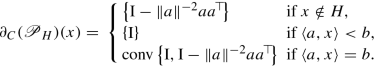
• d. Boxes. for some ℓ, u ∈ [−∞, ∞]ⁿ.

  We have

  

  and since the corresponding indicator function δ _D is separable, every element of $\partial _C(\operatorname {\mathscr P}_D)(x)$ is diagonal with (cf. Section §15.6.1a)

  

• e. Unit simplex. .

  By writing down the optimality conditions for the corresponding projection problem, one can easily see that

  $$\displaystyle \begin{aligned} \operatorname{\mathscr P}_D(x)=[x-\lambda\mathbf{1}]_+, \end{aligned} $$

  (15.106)

  where λ solves 〈1, [x − λ 1]₊〉 = 1. Since the unit simplex is a polyhedral set, we are dealing with a special case of Section §15.6.2b, where , b = 1, C = −I, and d = 0. Therefore, in order to calculate an element of the generalized Jacobian of the projection, we first compute $\operatorname {\mathscr P}_D(x)$ and then determine the set of active indices . An element $P\in \partial _B(\operatorname {\mathscr P}_D)(x)$ is given by

  

  (15.107)

  where |J| denotes the cardinality of the set J. Notice that P is block diagonal after a permutation of rows and columns.

• f. Euclidean unit ball. .

  We have

  

  and

  

  where w: = x∕∥x∥.

• g. Second-order cone. .

  Let $x\mathrel{\mathop:}= (x_0,\bar x)$, and for $w\in \mathbb {R}^n$ and $\alpha \in \mathbb {R}$ define

  

  (15.108)

  Then, $\partial _C(\operatorname {\mathscr P}_{\mathcal K})(x) {}={} \operatorname {conv}(\partial _B(\operatorname {\mathscr P}_{\mathcal K})(x))$ where, for $\bar w\mathrel{\mathop:}= {\bar x}/{\|\bar x\|}$ and $\bar \alpha \mathrel{\mathop:}= -{x_0}/{\|\bar x\|}$, we have [30, Lem. 2.6]

  

  (15.109)

• h. Positive semidefinite cone. $\mathcal S_+=\operatorname {S}_+(\mathbb {R}^{n\times n})$.

  For any symmetric matrix M it holds that

  

  (15.110)

  where is any spectral decomposition of M. This coincides with (15.93), as $\operatorname {\delta }_{\mathcal S_+}$ can be expressed as in (15.89), where h has the separable form (15.91) with $g=\delta _{\mathbb {R}_+}$, so that for $r\in \mathbb {R}$ we have

  

  (15.111)

  An element of $\partial _B\operatorname {\mathscr P}_{\operatorname {S}_+(\mathbb {R}^{n\times n})}(X)$ is thus given by (15.94).

15.6.3 Norms

• a. ℓ ₁ norm. g(x) = ∥x∥₁.

  The proximal mapping is the well-known soft-thresholding operator

  $$\displaystyle \begin{aligned} (\operatorname{prox}_{\gamma g}(x))_i {}={} \operatorname{{\mathrm{sign}}}(x_i)[|x_i|-\gamma]_+, \quad i=1,\ldots,n. \end{aligned} $$

  (15.112)

  Function g is separable, and thus every element of $\partial _B(\operatorname {prox}_{\gamma g})$ is a diagonal matrix, cf. Section §15.6.1a. Specifically, the nonzero elements are

  

  (15.113)

  We could also arrive to the same conclusion by applying the Moreau decomposition of Section §15.6.1b to the function of Section §15.6.2d with u = −ℓ = 1 _n, since the ℓ ₁ norm is the conjugate of the indicator of the ℓ _∞-norm ball.

• b. ℓ _∞ norm. g(x) = ∥x∥_∞.

  Function g is the convex conjugate of the indicator of the unit simplex D analyzed in Section §15.6.2e. From the Moreau decomposition, see Section §15.6.1b, we obtain

  $$\displaystyle \begin{aligned} \partial_C(\operatorname{prox}_{\gamma g})(x) {}={} \mathrm{I}-\partial_C(\operatorname{\mathscr P}_D)(\nicefrac x\gamma). \end{aligned} $$

  (15.114)

  Then, $\operatorname {\mathscr P}_D(\nicefrac x\gamma ) {}={} [\nicefrac x\gamma -\lambda \mathbf {1}]_+$ where $\lambda \in \mathbb {R}$ solves 〈1, [x∕γ − λ 1]₊〉 = 1. Let , then an element of $\partial _B(\operatorname {prox}_{\gamma g})(x)$ is given by

  

  (15.115)

• c. Euclidean norm. g(x) = ∥x∥.

  The proximal mapping is given by

  

  (15.116)

  Since $\operatorname {prox}_{\gamma g}$ is a PC ¹ mapping, its B-subdifferential can be computed by simply computing the Jacobians of its smooth pieces. Specifically, denoting w = x∕∥x∥ we have

  

  (15.117)

• d. Sum of Euclidean norms. $g(x)=\sum _{s\in \mathcal S}\|x_s\|$, where $\mathcal S$ is a partition of .

  Differently from the ℓ ₁-norm which induces sparsity on the whole vector, this function serves as regularizer to induce group sparsity [81]. For $s\in \mathcal S$, the components of the proximal mapping indexed by s are

  $$\displaystyle \begin{aligned} (\operatorname{prox}_{\gamma g}(x))_s {}={} (1-\gamma\|x_s\|{}^{-1})_+x_s.\end{aligned} $$

  (15.118)

  Any $P\in \partial _B(\operatorname {prox}_{\gamma g})(x)$ is block diagonal with the s-block equal to

  

  (15.119)

• e. Matrix nuclear norm. G(X) = ∥X∥_⋆ for $X\in \mathbb {R}^{m\times n}$.

  The nuclear norm returns the sum of the singular values of a matrix $X\in \mathbb {R}^{m\times n}$, i.e., $G(X)=\sum _{i=1}^m\sigma _i(X)$ (for simplicity we are assuming that m ≤ n). It serves as a convex surrogate for the rank, and has found many applications in systems and control theory, including system identification and model reduction [20,21,22, 41, 61]. Other fields of application include matrix completion problems arising in machine learning [62, 68] and computer vision [52, 76], and nonnegative matrix factorization problems arising in data mining [18].

  The nuclear norm can be expressed as G(X) = h(σ(X)), where h(x) = ∥x∥₁ is absolutely symmetric and separable. Specifically, it takes the form (15.91) with g = |⋅|, for which g(0) = 0 and 0 ∈ ∂g(0), and whose proximal mapping is the soft-thresholding operator. In fact, since the case of interest here is x ≥ 0 (because σ _i(X) ≥ 0), we have $\operatorname {prox}_{\gamma g}(x)=[x-\gamma ]_+$, cf. (15.116). Consequently, the proximal mapping of ∥X∥_⋆ is given by (15.98) with

  $$\displaystyle \begin{aligned} \varSigma_g(X)=\operatorname{diag}([\sigma_1(X)-\gamma]_+,\ldots,[\sigma_m(X)-\gamma]_+).\end{aligned} $$

  (15.120)

  For $x\in \mathbb {R}_+$ we have that

  

  (15.121)

  then $\partial _B(\operatorname {prox}_{\gamma G})(X)$ takes the form as in (15.99).

15.7 Conclusions

A forward-backward truncated-Newton method ( FBTN ) is proposed that minimizes the sum of two convex functions one of which Lipschitz continuous and twice continuously differentiable. Our approach is based on the forward-backward envelope (FBE), a continuously differentiable tight lower bound to the original (nonsmooth and extended-real valued) cost function sharing minima and minimizers. The method requires forward-backward steps, Hessian evaluations of the smooth function and Clarke Jacobians of the proximal map of the nonsmooth term. Explicit formulas of Clarke Jacobians of a wide variety of useful nonsmooth functions are collected from the literature for the reader’s convenience. The higher-order operations are needed for the computation of symmetric and positive semidefinite matrices that serve as surrogate for the Hessian of the FBE, allowing for a generalized (regularized, truncated-) Newton method for its minimization. The algorithm exhibits global Q-linear convergence under an error bound condition, and Q-superlinear or even Q-quadratic if an additional semismoothness assumption at the limit point is satisfied.

Appendix: Auxiliary Results

Lemma 1

Any proper lsc convex function with nonempty and bounded set of minimizers is level bounded.

Proof

Let h be such function; to avoid trivialities we assume that $\operatorname {{\mathrm {dom}}} h$ is unbounded. Fix $x_\star \in \operatorname *{\mathrm {argmin}} h$ and let R > 0 be such that . Since $\operatorname {{\mathrm {dom}}} h$ is closed, convex, and unbounded, it holds that h attains a minimum on the compact set $\operatorname {bdry} B$, be it m, which is strictly larger than h(x _⋆) (since $\operatorname {dist}( \operatorname *{\mathrm {argmin}} h,\operatorname {bdry} B)>0$ due to compactness of $\operatorname *{\mathrm {argmin}} h$ and openness of B). For x∉B, let $s_x=x_\star +R\tfrac {x-x_\star }{\|x-x_\star \|}$ denote its projection onto $\operatorname {bdry} B$, and let $t_x\mathrel{\mathop:}= \tfrac {\|x-x_\star \|}{R}\geq 1$. Then,

$$\displaystyle \begin{aligned} h(x) {}={} & h\big(x_\star+t_x(s_x-x_\star)) {}\geq{} h(x_\star)+t_x\big(h(s_x)-h(x_\star)\big) {}\geq{} h(x_\star)+t_x\big(m-h(x_\star)\big) \end{aligned} $$

where in the first inequality we used the fact that t _x ≥ 1. Since m − h(x _⋆) > 0 and t _x →∞ as ∥x∥→∞, we conclude that h is coercive, and thus level bounded. □

Lemma 2

Let $H\in \operatorname {S}_+(\mathbb {R}^n)$ with λ _max(H) ≤ 1. Then $H-H^2\in \operatorname {S}_+(\mathbb {R}^n)$ with

(15.122)

Proof

Consider the spectral decomposition for some orthogonal matrix S and diagonal D. Then, where $\tilde D=D-D^2$. Apparently, $\tilde D$ is diagonal, hence the eigenvalues of H − H ² are exactly . The function λ↦λ − λ ² is concave, hence the minimum in $\operatorname {eigs}(\tilde H)$ is attained at one extremum, that is, either at λ = λ _min(H) or λ = λ _max(H), which proves the claim. □

Lemma 3

For any γ ∈ (0, 2∕L _f) the forward-backward operator (15.22) is nonexpansive (in fact, $\frac {2}{4-\gamma L_f}$ -averaged), and the residual is Lipschitz continuous with modulus $\frac {4}{\gamma (4-\gamma L_f)}$.

Proof

By combining [2, Prop. 4.39 and Cor. 18.17] it follows that the gradient descent operator is γL _f∕2-averaged. Moreover, since the proximal mapping is 1∕2-averaged [2, Prop. 12.28] we conclude from [2, Prop. 4.44] that the forward-backward operator T _γ is α-averaged with $\alpha =\frac {2}{4-\gamma L_f}$, thus nonexpansive [2, Rem. 4.34(i)]. Therefore, by definition of α-averagedness there exists a 1-Lipschitz continuous operator S such that $T_\gamma =(1-\alpha )\operatorname {id}+\alpha S$ and consequently the residual is (2α∕γ)-Lipschitz continuous. □