A Data Science Approach to Predict the Impact of Collateralization on Systemic Risk

Abstract

In this chapter, we simulate and analyze the impact of financial regulations concerning the collateralization of derivative trades on systemic risk—a topic that has been vigorously discussed since the financial crisis in 2007/08. Experts often disagree on the efficacy of these regulations. Compounding this problem, banks regard their trade data required for a full analysis as proprietary. We adapt a simulation technology combining advances in graph theory to randomly generate entire financial systems sampled from realistic distributions with a novel open-source risk engine to compute risks in financial systems under different regulations. This allows us to consistently evaluate, predict, and optimize the impact of financial regulations on all levels—from a single trade to systemic risk—before it is implemented. The resulting data set is accessible to contemporary data science techniques like data mining, anomaly detection, and visualization. We find that collateralization reduces the costs of resolving a financial system in crisis, yet it does not change the distribution of those costs and can have adverse effects on individual participants in extreme situations.

1 Introduction

Counterparty credit risk (CCR) is the risk of suffering a loss when a contracting party defaults before satisfying its obligations. While banks and financial institutions have been well aware of the CCR in classical business lines like loans for centuries, the credit risk component in derivative trades has gained recent attention. Since the 2008 crisis, markets can no longer assume that the credit risk in a derivative with a bank is zero—even if it is AAA rated. As the volume of the over-the-counter (OTC) derivative business alone exceeds $20,701 billions of the US dollars,¹ it has been suggested that the inherent credit risk now poses a significant threat to the system. Indeed, a number of financial regulations have been enacted aimed at reducing this credit risk. A key feature of these regulations is that they provide strong incentives (and increasingly the obligation) to collateralize derivative trades, i.e., post and receive capital.

It is obvious that a counterparty² that receives collateral for its derivative trades has a lower CCR exposure than a counterparty that does not. However, it is less obvious to show that the introduction of collateralization reduces the systemic risk in a financial system as a whole. Since the turmoil following the collapse of Lehman Brothers in the 07/08 crisis, there has been a vibrant discussion on how to improve financial regulation to avoid another crisis in the future. This crisis has not only questioned the soundness of the current regulation but also the process on how to decide what regulations to implement. Although a decade has passed by now, there is still little consensus on how to evaluate, predict, and optimize financial regulation, that is:

• 1. Evaluate: Has the regulation implemented since the financial crises reduced systemic risk or not?

• 2. Predict: How can we predict the impact of a financial regulation before it is implemented on the real financial system?

• 3. Optimize: How can we find the best possible financial regulation?

Data science provides new solutions to measuring and predicting systemic risk in financial systems. It is the aim of this article to use these new technologies to develop a framework in which these questions can be answered quantitatively and systematically and to apply this technology to prominent regulations regarding the collateralization of derivative trades.

The rest of this chapter is organized as follows: In Sect. 2, we provide a framework to coherently extend enterprise-level risk metrics to a systemic level using a graph model, in which the nodes represent individual banks and the links represent trade relations. We present a purely graph theoretic technique on how to aggregate the risks arising in those trades to a counterparty and to a systemic level employing a weighted multivariate version of the in/out degree. In Sect. 3, we present in detail our data science approach to predict the impact of a regulation on systemic risk using recent advances in random graph generation and a novel open-source risk engine (ORE). We present our results in Sect. 4 and conclude with further research plans in Sect. 5.

The analysis validates that collateralization does indeed reduce systemic risk; it does not, however, change the distribution of risk in a system. The analysis also illustrates that validation depends on the metric chosen to quantify systemic risk. We find that while on a macro-level, the impact of collateralization is unambiguously risk reducing, and it can increase the risk stemming from individual netting sets in extreme cases.

1.1 State of the Art

One of the main methods currently used to evaluate financial regulation is expert judgment (of course based on quantitative studies providing a snapshot of data of the current financial system). The main disadvantage of expert judgment is that different experts have different opinions. If experts do not even agree in their judgment on whether or not the changes in regulations so far are improvements, there is little hope to answer the question of how to find an optimal financial regulation with that method.

Data science and ultimately machine learning offer a viable alternative by tackling some of the root causes why experts fail to agree:

• 1. Micro- vs. Macro-regulation: In financial economics, the impact of a financial regulation is currently studied either on the micro-prudential level, which considers only a single individual bank with its trades in all its detail, but ignores systemic effects, or on the macro-prudential level, which considers only systemic effects, but ignores most of the implications on individual banks, see Fig. 1. As financial regulations heavily affect the financial system on both levels—sometimes in opposite ways—this gap makes it very difficult to arrive at consistent answers.

• 2. Inconsistent metrics and unclear definitions: This gap is particularly visible when reviewing risk metrics. On the micro-prudential level, there are very well-defined types of risk, for instance market risk (suffering a loss due to adverse market movements), counterparty credit risk (suffering a loss due to a default of a business partner), liquidity risk (running out of money), or model risk (models used to quantify any of the previous risks are wrong). Furthermore, there are standardized metrics to measure them like Value-at-Risk, Effectivized Expected Positive Exposure (EEPE), Liquidity Coverage Ratio, or a Basel Traffic Light Test. Not only are these metrics standardized, their use is enforced globally by regulators.

  On the macro-prudential level, there is not even a clear definition on what systemic risk means or how it should be measured. In [7], the US Office for Financial Research discusses 31 metrics of systemic risk. Most of these metrics focus on the analysis of market data like housing prices or government bonds and their correlations. For instance, [6] use principal components analysis (PCA) and Granger causality to study the correlations between the returns of banks, asset managers, and insurances. Unfortunately, most of those macro-prudential metrics are unsuited to guide decision-making bodies or regulatory interventions—precisely because their micro-prudential nature remains unclear (with CoVaR, which relies on a quantile of correlated asset losses, being a notable exception, see [1]).

  This incoherence in metrics yields to incompatible views when evaluating the impact of financial regulations. One of the key strengths of a data science approach is that it enforces a consistent quantification of features and transparent evaluation metrics.

• 3. Lack of Data: While macro-economic data of the financial markets is easily available, even macro-economic data on the financial system is often not publicly available, Cont et al. were able to obtain macro-level data of aggregate interbank exposures of the Brazilian banking system during 2007/08 from the Brazilian Central Bank and adopt a graph model to describe the interconnectedness of the system and to estimate the impact that an increase in capital requirements has on those interbank exposures, see [10].

  While those analyses are very interesting on a macro-prudential level, they cannot predict the impact of financial regulations on a micro-prudential level, because their impacts depend on a banks’ individual trades. However, all banks regard their trade data as proprietary.

Fig. 1

Using data science to close the gap between micro- and macro-prudential regulation

1.2 Method and Approach

The lack of data is a nontrivial practical problem for the calibration and backtesting of any model of systemic risk. Notice that even if one would obtain the trade data of the entire financial system as of today and test the impact of a regulation with the aim of guiding a decision-making process, this would still not guarantee that its implementation has the desired effects. The regulations regarding Initial Margin are a consequence of the financial crisis in 2007/08, but the last phase-in date for Initial Margin is currently set at 2020. A lot of the trades that existed in 2007 will have matured in 2020. Therefore, it is imperative to make sure that the regulation is future proof and has the desired effect not only on the current financial system but ideally also on all possible future versions of it.

Our approach is to randomly generate financial systems sampled from realistic distributions and simulate their future evolution under different regulatory regimes. The key tool is a systemic risk engine, which combines a novel open-source risk engine with graph theoretic models. This allows us to consistently calculate the risks of all individual banks and the system as a whole, hence bridging the gap between micro- and macro-prudential economics.³

The systemic risk engine uses the following key components and steps, see also Fig. 2:

• 1. Graph Model—Trade Relations: Any financial system at a fixed point in time can be modeled using an undirected graph, where the nodes represent the banks and the links represent the trade relations between them, see Definition 1 for details and Fig. 3 for a simplified example.⁴

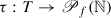
• 2. Graph Model—Risk Metrics: The exposures stemming from the trade relations in a financial system can be represented as a directed graph where the nodes again represent the same banks and the arrows represent the risk induced from the tail to the head, see Definition 2 for the details and Fig. 4 for an example. The standardized micro-prudential metrics give rise to weight functions on the arrows, which quantify the risks stemming from the trade relations, for instance EEPE for counterparty credit risk. These can then be aggregated consistently to systemic versions using weighted in and out degrees, see Definition 3 and Definition 4 for details.

• 3. Financial System Generation: We randomly generate trade relation graphs G ₁, …, G _s, of financial systems sampling from the distributions found in [10], see Fig. 5 for an example. This is achieved using the configuration erase model from the Python library networkx based on [5, 8, 16], see component I in Fig. 2.

• 4. Systemic Risk Engine: In order to compute the individual risks in each banks’ portfolio, we propose to use ORE, a novel open-source risk engine, see [19], which is based on QuantLib and implemented in C++. We extend this to a systemic risk engine, which computes not only the risk of any individual bank in the system but also aggregated systemic risk metrics, see component IV in Fig. 2. The main task is to automate entering all the generated financial systems into OREs XML configuration files, which is done using the Python library lxml.

• 5. Risk Graph Generation: Technically, a financial regulation can be implemented into the systemic risk engine as part of its input configuration, see component III of Fig. 2. Therefore, we can simulate the impact of a proposed financial regulation $R_{ \operatorname {\mathrm {prop}}}$ compared to a base regulation $R_{ \operatorname {\mathrm {base}}}$ by running the systemic risk engine on each of the financial systems G ₁, …, G _s under regulation $R_{ \operatorname {\mathrm {base}}}$ as well as $R_{ \operatorname {\mathrm {prop}}}$, see components IV and V of Fig. 2.

• 6. Classification, Data Mining, and Visualization: In a last step, we aggregate the generated data to allow hypothesis testing on whether or not the impact of $R_{ \operatorname {\mathrm {prop}}}$ over $R_{ \operatorname {\mathrm {base}}}$ has reduced systemic risk, see component VI of Fig. 2. In addition, we use this raw data for data mining techniques such as anomaly detection to identify corner cases, in which $R_{ \operatorname {\mathrm {prop}}}$ has adverse effects or fails.

Fig. 2

IT architecture of data science solution

Fig. 3

Trade relations: the nodes represent the banks, the links represent the trade relations, and the labels on the links represent the trade or portfolio IDs

Fig. 4

Exposures: the nodes represent the same banks as in Fig. 3, the arrows represent that risk is induced from the bank on the tail onto the bank on the head, the weights on the arrows quantify that risk, and the percentages in the nodes represent the share of risk induced by that bank

Fig. 5

A randomly generated trade relation graph

It seems obvious to bridge the gap between micro- and macro-prudential regulation by understanding the macro-prudential impact of a financial regulation via an aggregation of all the micro-prudential impacts on all banks, see again Fig. 1. The complexity of the system and of each of its banks as well as the large number of banks has made such an approach intractable for the traditional methods in financial economics. We believe that the current level of data science and risk management technology makes this bottom-up approach feasible for the first time. The approach has the advantage that it allows to understand the micro-prudential impact not only on one entity but on all of them simultaneously and systematically.

Notice that bridging a gap between a micro-perspective and a macro-perspective using data science to understand the macro-perspective as an aggregation of all micro-perspectives and organizing them in a graph model could in principle be applied to other domains as well, for instance payment systems, elections, or sentiment analysis.

2 A Graph Model of Financial Systems and Systemic Risk Metrics

A financial system can be modeled as a graph,⁵ where the nodes represent the counterparties. Two counterparties are connected by an (undirected) edge if and only if they are conducting business with each other. The nodes as well as the edges can be enriched with additional data regarding the counterparties or the trade relations.

2.1 Trade Relation Graph

We capture this by the following formal definition, see Fig. 3.

Definition 1 (Financial System)

A financial system $\operatorname {\mathrm {FS}}=(B, T, \tau )$ is an undirected graph G = (B, T) called trade relation graph together with a trade data function τ, where:

• B is the set of nodes in the graph representing the banks.

• T is the set of (undirected) edges in the graph representing the trade relations between the banks. Two banks b ₁ ∈ B and b ₂ ∈ B are connected by an edge if and only if they have at least one trade with each other.

• τ : T → Y  is a trade data function, which to each trade relation t assigns additional trade relation data τ(t) (for instance a list of trade IDs) in some data space Y .

Optionally, this can be enriched to (B, T, β, τ), where:

• β : B → X is a node data function, which assigns each bank b ∈ B additional data β(b) (for instance its core capital) in some data space X.

In Fig. 3, we see an example of a financial system, where six banks (labeled A–F here) are trading bilaterally with each other in five trade relations. The trade data function τ assigns to each trade relation t the ID of a trade (IRS1 for instance stands for an Interest Rate Swap). While in this example, every trade relation only consists of one trade, banks often have many trades with each other.⁶ While it is possible (both mathematically and technically) to assign more data than just a list of trade IDs to a trade relation, we stick to this simple trade data function for now. Optionally, one can supply this example with a node data function β, which is not shown in Fig. 3. A meaningful example of a function β is to assign to each bank b its core capital (or core capital ratio).

2.2 Risk Graph

Each trade in a trade relation imposes various types of risks (as well as rewards) on potentially both banks, which can be computed in various metrics by means of mathematical finance. By computing a fixed set of risk metrics for all trade relations in a trade relation graph, we obtain a graph that captures the risks between all the various banks in the system, see Fig. 4. Formally, we define this as follows:

Definition 2 (Risk Graph)

Let $\operatorname {\mathrm {FS}}=(B, T, \tau )$ be a financial system as in Definition 1 (optionally enriched by a node data function β). A weighted directed graph is called a risk graph associated to $\operatorname {\mathrm {FS}}$, where:

• B is the set of nodes in the graph representing the banks (i.e., $\operatorname {\mathrm {FS}}$ and have identical nodes).

• A is the set of directed edges (often called arrows) in the graph . We add an arrow from a bank b ₁ ∈ B to a bank b ₂ ∈ B if and only if b ₂ is exposed to some form of risk from b ₁ as a consequence of their trades.

• is a multivariate weight function on the arrows quantifying the risks attached to each arrow measured in k metrics.

While the nodes in the trade relation graph and in the risk graph are the same, the edges are not. Each undirected edge in $\operatorname {\mathrm {FS}}$ gives rise to one or two edges in . This is because there are trades like Interest Rate Swaps that induce risk from one counterparty to another and vice versa. In this case, we see two arrows between the counterparties that go in opposite directions, which in Fig. 4 is the case for all trade relations. Notice that there are also trades like FX Options where risk is induced in one direction only. On the arrows in Fig. 4, we only see one number, so k = 1, and the weight function chosen here is , i.e., if a = (b ₁, b ₂), then w(a) denotes the $\operatorname {\mathrm {EEPE}}$ that b ₂ receives from b ₁. Another example could be the $\operatorname {\mathrm {PFE}}$ over a certain time horizon at a fixed quantile α (analogous to the US stress testing). Here, $\operatorname {\mathrm {EEPE}}$ stands for Effectivized Expected Positive Exposure and $\operatorname {\mathrm {PFE}}$ for Potential Future Exposure. These are standardized metrics to express risks in derivative portfolios, see [17, Sect. III] for a detailed discussion.

The weight function w in the risk graph associates a weight to the arrows. As banks often trade with many counterparties, we want to aggregate this information into a weight function on the nodes, i.e., the banks themselves. There is a purely graph theoretic procedure that extends a weight function on arrows to a weight function on nodes. As this method is less standard, we give the following definition.

Definition 3 (Weighted In/Out Degree)

Let G = (V, E, w) be a directed graph with nodes V , edges E, and a weight function . In case k = 1, for each vertex v ∈ V , the quantities:

$$\displaystyle \begin{aligned} w^{-}(v) := \sum_{\substack{e \in E \\ e\text{ ends at }v}}{w(e)}, && w^{+}(v) := \sum_{\substack{e \in E \\ e\text{ starts at }v}}{w(e)} \end{aligned} $$

(1)

are called the weighted in/out degree. Let w(G) :=∑_{e ∈ E}w(e) be the total weight in the system. The quantities:

(2)

are called weighted relative in/out degree. In case the weight function is multivariate, the weighted in/out degree and the relative weighted in/out degree are defined using Eqs. (1) and (2) in each component.

Intuitively, w ^±(v) is the total weight received respectively induced by v into the graph G. Notice that in case k = 1 and w ≡ 1, we have w ^±(v) =deg^±(v), i.e., the weighted in/out degree is the ordinary in/out degree, which just counts the number of incoming respectively outgoing edges. Any of the quantities:

(3)

are -real-valued metrics that capture the total amount of weight in the graph and its concentration.

2.3 Systemic Risk

Applying these graph theoretic concepts to systemic risk is straightforward.

Definition 4 (Systemic Risk)

Let be a risk graph as in Definition 2. Extend the weight function on the arrows to a weight function using the weighted in/out degree from Eq. (1). We also define via Eq. (2). We regard any of the quantities in Eq. (3) as a metric of systemic risk.

As any metric that measures risk in a trade relation between two counterparties can be used as a weight function in a risk graph, we have produced a general procedure how to construct a systemic risk metric from that.

An example for such a metric is $w= \operatorname {\mathrm {EEPE}}$. In that case for each bank b, the quantity $\operatorname {\mathrm {EEPE}}^+(b)$ can be thought of as the cost of resolution if b defaults (like a loss given failure, but not a probability of failure). The quantities ρ ⁺(b) are a metric that quantifies the concentration of these costs of resolution in the system.

3 Simulation Technology

In order to predict the impact of a financial regulation on systemic risk, we randomly generate financial systems as trade relation graphs, like the one shown in Fig. 3. For all netting sets containing all the trades in all the financial systems, we then compute risk metrics under different regulations. Using this data, we populate risk graphs like Fig. 4 for each regulation. Finally, we aggregate all these graphs to come to a conclusion on how a regulation impacts systemic risk. An overview of the technologies used in these various steps and their interactions is shown in Fig. 2. We will discuss the key challenges in this section.

3.1 Generation of Random Trade Relation Graphs

In order to generate random trade relation graphs like Fig. 3, various distributional choices have to be made.

3.1.1 Nodes

Generating the number of nodes is straightforward by choosing either a fixed value or drawing from a uniform distribution between an upper and lower bound.

3.1.2 Edges

How to randomly generate the edges such that the resulting trade relation graph forms a realistic financial system? Ideally, one should sample those from empirical data, but the trade relations in the real financial system are top secret. However, in [10] a statistical analysis of the macro-exposures in the Brazilian banking system has been performed using aggregated anonymized data provided by the Brazilian central bank. Due to this analysis, it is known that the degrees of the nodes in the trade relation graph follow approximately a Pareto distribution. Therefore, the problem can be split up into sampling a Pareto distributed sequence {d ₁, …, d _n}, where n is the number of nodes in the graph, and second by creating a graph out of this sequence. While the first step is straightforward, the second is not.

Generating random graphs with a degree sequence prescribed from a given distribution is a hard problem in discrete mathematics. For Poisson distributed degree sequences, a solution has been developed by Erdős and Rényi in the 1960, see [12, 13]. With the advances of the WWW and social networks, generating random graphs with degree sequence sampled from an arbitrary given distribution became a useful tool. Therefore, substantial theoretical work as well as the search for efficient algorithms has been invested into this problem. We use the erased configuration model as implemented in the Python library networkx and described in [16]. Further details can also be found in [5, 8]. For random number generation, we use the Python library numpy.random.

3.1.3 Trades

Once a trade relation has been generated, the portfolio between the banks attached to this relation has to be populated with trades. For the purpose of this text, we keep it simple and choose a number k of trades, uniformly distributed between a fixed upper and lower bound, and then draw k times without replacement from a list of trade IDs. To generate the trades behind these IDs, we start with an FX Forward (EUR vs. USD) with a uniformly distributed maturity of up to 5 years, a uniformly distributed domestic amount between 100k and 100mn and a log-normally distributed strike rate, and also with an Interest Rate Swap (fixed vs. floating) with a uniformly distributed maturity of up to 10 years, a uniformly distributed notional between 100k and 100mn, and a uniformly distributed fixed rate between 0.01% and 5%. The choice between a Forward and the Swap as well as the sides of the trades are Bernoulli distributed with probability 0.5. We assume that all trades between two counterparties are in precisely one netting set.

3.2 The Open-Source Risk Engine (ORE)

Computing the exposure in even in just a single netting set of derivative trades is a hard problem in mathematical finance. The risk department of a bank invests substantial resources into developing and maintaining a risk management system capable of computing the banks exposure—in particular, if the bank chooses to use its own internal models. As those risk management systems are proprietary, they cannot be used for the purpose of this text.

Therefore, we use the Open-Source Risk Engine (ORE), an open-source software, which performs risk management computations like a production system in a bank. It has been released by Quaternion Risk Management in 2015 as part of the Open-Source Risk initiative, see [19]. ORE models the risk in a derivative trade from the perspective of a single bank. Given the banks’ portfolio, market data, and some additional configuration files, it projects the value of the trades into the future using a Monte Carlo simulation based on complex stochastic modeling of the risk factors. A detailed description of these risk factor models can be found in [14]. In case of a collateralized netting set, ORE also consumes parameters that specify the details of a netting agreement and simulates the value of collateral. This is a nontrivial matter. In particular, forecasting the IM is still subject to current research, see [3, 9, 11, 15].

3.3 Configuration and Aggregation

Each generated trade relation graph and each regulation has to be entered into OREs XML configuration before a run can be kicked off. This is realized via a Python script using lxml. After the run, OREs output consists of csv files containing all the risk metrics. We use pandas to extract those from the files and populate the risk graphs like Fig. 4. This puts us in a position to compute statistics on the risk metrics in the various graphs under various regulations.

4 Results: Impact of Collateralization on Systemic Risk

In this section, we apply the simulation technology described in Sect. 3 to study the impact of various collateralization regulations on systemic risk. The value of a derivative contract stems from future cashflows, which are not yet settled. If no collateral is exchanged, both parties are fully exposed to each other’s credit risk (REG_1). To mitigate that risk, parties can exchange Variation Margin (VM) to cover the current exposure, i.e., the immediate loss suffered by the surviving counterparty on default (REG_3). This still does not reduce the exposure to zero as the surviving counterparty will need some time to close out the position. To mitigate the potential exposure caused by this gap, parties can exchange Initial Margin (IM) on top of the Variation Margin (REG_4). A detailed description of these three regulatory regimes can be found in [17, Sect. II].

In [17, Sect. V], we presented a case study, which analyzes the impact of these three different regulatory regimes on the financial system with the structure depicted in Fig. 3. We found while increasing collateralization decreases systemic risk measured in $\operatorname {\mathrm {EEPE}}$ (respectively, $\operatorname {\mathrm {EEPE}}+$, see Definition 3), i.e., the total cost of resolving a failed system decreases with the amount of collateral. However, collateralization has only little effect on the concentration of these costs (i.e., the associated ρ +  does not change much).

We now use the simulation technology described in Sect. 3.1 to generate 10 financial systems with 30–50 counterparties and trade relations, which are approximately Pareto distributed. This results in 2360 trades in total. These are faced from two sides, which yields 4720 technical trades in 1378 netting sets in ORE. We compute the $\operatorname {\mathrm {EEPE}}$ under the regulatory regimes 1), 3), and 4) using 500 Monte Carlo paths. Regulatory regime 2) is omitted, because if one sets a global threshold, the result would depend on an arbitrary choice on whether or not the netting set exposures are distributed above or below that threshold, which is unrealistic. In Fig. 6, we can see that under regime 3), i.e., the full VM collateralization, the total $\operatorname {\mathrm {EEPE}}$ reduction is at about 71%, and under regime 4), i.e., the VM & IM collateralization, the reduction is at about 93%. The average does not exhibit any outliers among the 10 financial systems analyzed, see Fig. 7.

Fig. 6

Total reduction of $\operatorname {\mathrm {EEPE}}$

Fig. 7

Average relative reduction of total $\operatorname {\mathrm {EEPE}}$ in the various financial systems

On a macro-level, these numbers confirm unambiguously that the impact of any collateralization yields to a reduction in risk. As a byproduct of the simulation, we obtain exposure data of 1378 netting sets, which we can now mine to gain insight into all micro-impacts of the various regulations.

In Fig. 8, we see the distribution of relative reductions in $\operatorname {\mathrm {EEPE}}$ of the various netting sets when comparing REG_1 (uncollateralized) with REG_3 (VM collateralized). While most of the netting sets show a significant relative reduction in exposure, we can see that some of them also show a significant relative increase in exposure. The explanation for this is as follows: Assume that bank A has trades in a netting set with bank B. These trades are deeply out of the money for bank A, meaning that the markets have moved into bank B’s favor. Then, the uncollateralized exposure for bank A is very low.⁷ Under VM collateralization however, as the trades are deeply in the money for bank B, bank B will call bank A for variation margin. Bank A will then pay the variation margin to bank B, where it is exposed to the default risk of B, because B might rehypothecate this variation margin. In some situations, this is resulting in higher exposure under VM collateralization than under no collateralization. We see that on a micro-level, VM collateralization can have an adverse effect in rare cases of netting sets, which are deeply out of the money.

Fig. 8

Histogram of relative reduction in $\operatorname {\mathrm {EEPE}}$ over all netting sets (197 out of 1378 have more than 150% increase and are not shown, 29 of those have zero uncollateralized $\operatorname {\mathrm {EEPE}}$). Mean:− 57.42%, SD: 38.33%

Initial Margin cannot be rehypothecated and therefore, posted Initial Margin is not treated as being at risk.⁸ In Fig. 9, we see the relative reductions in $\operatorname {\mathrm {EEPE}}$ of the various netting sets when comparing REG_3 (VM collateralization) vs. REG_4 (VM & IM collateralization). Here, we can see that the effect of the additional IM overcollateralization unambiguously reduces the exposure further.

Fig. 9

Histogram of relative reduction in $\operatorname {\mathrm {EEPE}}$ over all netting sets (0 out of 1378 have more than 150% increase and are not shown, 0 of those have zero VM collateralized $\operatorname {\mathrm {EEPE}}$). Mean: − 85.78%, SD: 20.76%

When comparing REG_1 (uncollateralized) vs. REG_4 (VM & IM collateralization) directly, we can see in Fig. 10 that the reduction in exposure is larger and distributed more narrowly compared with just the VM collateralization, see Fig. 8. There are still some netting sets left, which show an increase which is due to posted variation margin. However, this increase is smaller as under REG_3 as it is mitigated by the additional IM collateral.

Fig. 10

Histogram of relative reduction in $\operatorname {\mathrm {EEPE}}$ over all netting sets (69 out of 1378 have more than 150% increase and are not shown, 29 of those have zero uncollateralized $\operatorname {\mathrm {EEPE}}$). Mean: − 83.83%, SD: 34.44%

It should be noted that while the increases in exposure we see in Figs. 8 and 10 are large in relative terms, they are actually quite small in absolute terms, see Fig. 11, where we compute the total increases and decreases in $\operatorname {\mathrm {EEPE}}$ of all the netting sets separately.

Fig. 11

Total increases and decreases in $\operatorname {\mathrm {EEPE}}$ of all netting sets between the various regimes

4.1 Jupyter Dashboard

To interactively explore the above results further, we developed a Jupyter dashboard,⁹ see Fig. 12, using the jupyter_dashboards extension. Data on various financial systems and effects from various collateralization regulations outputted from the systemic risk engine is imported using pandas. The data is manipulated into proper forms for graphing purposes primarily using pandas and numpy. The trade relations and risk graphs are assembled using the erased configuration model from networkx and visualized using the visJS2jupyter module. The size of each node corresponds to the share of risk induced by the counterparty, while the width of the in-edges and out-edges quantifies the risk received respectively induced by the counterparty.

Fig. 12

Visualization of data outputted from systemic risk engine in Jupyter notebook dashboard. Depicts trade relations and risk graphs for various financial systems/regimes (top left) along with impact on risk within system (top right) and on individual counterparties measured in absolute terms (bottom left) and relative terms (bottom right). Can be configured and visualized with different regulations imposed

The remaining graphs are plotted using bqplot. The interactive menu is created using elements from the ipywidgets module that interact directly with elements within the notebook. The various financial systems and regulations can be chosen using dropdown menus with the option to switch between the trade relation and risk graphs. Javascript is employed to allow for dynamic execution of cells within the notebook and recreation of the graphs. Animations built into bqplot allow for seamless transitions across configurations, while the networkx graphs are regenerated upon each execution.

5 Synopsis

Our results can be summarized as follows:

• 1. Collateralization reduces the costs of resolution drastically,¹⁰ see Fig. 6. In that sense, it reduces systemic risk.

• 2. The case study however suggests that collateralization does not change the distribution of these costs in the system, see [17, Sect. V].

• 3. The data mining exercise makes visible that in rare cases of netting sets, which are deeply out of the money, VM collateralization can actually cause an increase in exposure, which can be large in relative terms, but is small in absolute terms, see Figs. 8 and 11.

Notice that these results are an interplay of the aggregated macro-exposures and a systematic analysis of all micro-exposures, which would not be possible outside of the present framework.

Regarding practical applicability of this research, any bank b knows its own $\operatorname {\mathrm {EEPE}}^-(b)$ and has to report this quantity to the regulator. It is reasonable to assume that it also knows its $\operatorname {\mathrm {EEPE}}(b,b')$ for any other counterparty b′ it does business with. (Especially for large complex banks, it is reasonable to assume that they can compute their own $\operatorname {\mathrm {EEPE}}^+(b)$ as well.) A regulator who would collect this information from all banks in the system could actually compute a graph like Fig. 4 representing the exposures in the real financial system as of today.

The research outlined in this chapter can be expanded into several directions.

Large-Scale Simulation

The results from Sect. 4 we obtained by running the simulation technology described in Sect. 3 on a client desktop machine. We plan to deploy this on a cold environment and run a larger-scale simulation.

Capitalization and Central Clearing

The $\operatorname {\mathrm {EEPE}}^+(b)$ of a bank b should be thought of as a measure of loss given failure, not a probability of failure. A bank with a large $\operatorname {\mathrm {EEPE}}^+(b)$ can actually still be very safe, if it has also large capital reserves. The key to take this into account is to add a capital adequacy ratio function as a node data function in Definition 1 and to add as an additional risk metric to the edges of the risk graph in Definition 2 (and then also to the nodes via the procedure described in Definition 4). The core capital of each bank can then be computed from that. This allows us to model a bank failure due to market risk, for instance by using the criterion:

$$\displaystyle \begin{aligned} \operatorname{\mathrm{CC}}(b) < \operatorname{\mathrm{VaR}}_{q}(b), \end{aligned} $$

(4)

where $\operatorname {\mathrm {VaR}}_q$ is the Value at Risk at some confidence level q. It also allows us to model a bank failure due to credit risk, for instance using the criterion:

$$\displaystyle \begin{aligned} \operatorname{\mathrm{CC}}(b_1) < \operatorname{\mathrm{EEPE}}((b_1,b_2)). \end{aligned} $$

(5)

By increasing the confidence level q further and further and labeling a bank as defaulted if either Eqs. (4) or (5) is satisfied, one can study the collapse of the whole system. In particular, one can study how a default of one counterparty causes chain reaction of defaults. The values of q at which default events occur can be interpreted as p-values of the hypothesis that the system is safe. We believe this framework to be particularly suited to study the regulation around central clearing in a similar fashion.

Agents-Based Creation of Trade Relation Graphs

Recall from Sect. 3.1 that we are currently generating the trade relations such that the degrees are approximately Pareto distributed, because this is in line with empirical data from [10]. If we prescribe the degrees, we obviously cannot get any insight into why those trade relations are formed. Therefore, we propose to enhance this by adding a trading strategy to the node data in Definition 1 for each bank. During the simulation, the banks would then trade based on that strategy and the evolution of the market and form those trade relations dynamically. It would be interesting to study under what conditions this produces Pareto distributed trade relations. As a byproduct, this enables studying the systemic market risks in trading strategies. What happens for example if everybody is trend following?

Derivative Market vs. Money Market

In the current example, only the derivative business is considered. However, there is also an inherent credit risk in the classical money market. The financial regulation on collateralization has a significant impact on the interplay between the two: Unlike Variation Margin, the Initial Margin cannot usually be rehypothecated (that means you cannot reuse the Initial Margin you receive from one counterparty to post your Initial Margin to another). Raising the necessary funds to post Initial Margin will increase the business in the money markets and it would be interesting to test the hypothesis that this increases the systemic credit risk in the money market in a similar fashion. In that case the trade-off between the reduction of credit risk in the derivative market and the increase of credit risk in the money market should be further examined. Imagine a situation where a counterparty A hedges a trade it has sold to counterparty B by buying a reversed trade from counterparty C. Although A has zero market risk, it has to post Initial Margin twice, namely to B and C. If A borrows this Initial Margin directly or indirectly from B or C, the reduction in overall credit risk across both markets will be a lot lower.

Initial Margin and Funding Costs

The reduction in EEPE in the derivative business comes at the cost of funding the collateral, in particular the Initial Margin. It is to be expected that these costs will be significant. On the other hand, the reduction in $\operatorname {\mathrm {EEPE}}$ yields to a reduction in , which yields to a reduction in the cost of capital. Therefore, it would be interesting to study the trade-off between the reduction in the cost of capital and the increase in funding costs. There are already various standardized metrics, called XVAs, to measure funding costs. In particular, the Margin Value Adjustment (MVA), which captures the additional funding costs due to Initial Margin, contributes significantly. Studying the levels, evolution, and distribution of Variation Margin and Initial Margin and the associated XVAs as part of a case study as well as systemic versions of that would enable a quantitative evaluation of the trade-off.

Credit Risk vs. Liquidity Risk vs. Market Risk vs. Model Risk

While the reduction of credit risk in Fig. 6 is very convincing, one should keep in mind that EEPE, the metric we use to quantify systemic risk, is a metric that captures Counterparty Credit Risk only. However, this is not the only source of risk in a financial system. Therefore, it would be more precise to say that collateralization reduces systemic credit risk. It is very reasonable to assume that pulling large amounts of money out of a financial system due to Initial Margin increases the liquidity risk in that system. Therefore, testing the hypothesis that collateralization increases systemic liquidity risk in a similar fashion and again study the trade-off between the two would be enlightening. We believe that the key to understand the link between credit risk and liquidity risk lies in a detailed analysis of the XVAs. While quantifying liquidity risk is difficult, it should be pointed out that value at risk (VaR), a standard metric to measure market risk—the most obvious source of risk—has a systemic analogue, namely CoVaR, see [1]. Finally, model risk can be added as well. This would allow us to study if for instance the increasing standardization of models increases or decreases the risk of system-wide model failures. What happens if everybody uses the same model and there exists a market condition under which it fails at one bank? It would be prudent to have a comprehensive simulation that studies the impact of collateralization on all these sources of risk and systemic risk.

References

Adrian, T., Brunnermeier, M.K.: CoVaR. Am. Econ. Rev. 106(7), 1705–1741 (2016)
Andersen, L., Pykhtin, M., Sokol, A.: Does Initial Marign Eliminate Counterparty Risk?, risk.net (May 2017)
Anfuso, F., Aziz, D., Giltinan, P., Loukopoulos, K.: A Sound Modelling and Backtesting Framework for Forecasting Initial Margin Requirements, SSRN Pre-print (2016)
Bales, M., Johnson, S.: Graph theoretic modeling of large-scale semantic networks. J. Biomed. Inform. 39(4), 451–464 (2006)
Bayati, M., Kim, J.-H., Saberi, A.: A sequential algorithm for generating random graphs. Algorithmica 58(4), 860–910 (2010)
Billio, M., Getmansky, M., Lo, A.W., Pelizzon, L.: Econometric Measures of Systemic Risk in the Finance and Insurance Sectors. NBER Working Paper 16223, NBER (2010)
Bisias, D., Flood, M., Lo, A.W., Valavanis, S.: A Survey of Systemic Risk Analytics. Office of Financial Research, Working Paper #0001 (January 5, 2012)
Britton, T., Deijfen, M., Martin-Löf, A.: Generating simple random graphs with prescribed degree distribution. J. Stat. Phys. 124(6), 1377–1397 (2006)
Caspers, P., Lichters, R.: Initial Margin Forecast–Bermudan Swaption Methodology and Case Study (February 27, 2018). Available at SSRN: https://ssrn.com/abstract=3132008
Cont, R., Moussa, A., Santos, E.: Network structure and systemic risk in banking systems. In Fouque, J., Langsam, J. (ed.): Handbook on Systemic Risk, pp. 327–368. Cambridge University Press, Cambridge (2013). https://doi.org/10.1017/CBO9781139151184.018
Caspers, P., Giltinan, P., Lichters, R., Nowaczyk, N.: Forecasting initial margin requirements–a model evaluation. J. Risk Manage. Financ. Inst. 10(4), 365–394 (2017)
Erdős, P., Rényi, A.: On random graphs. Publ. Math. 6, 290–297 (1959)
Erdőos, P., Rényi, A. On the evolution of random graphs. Publ. Math. Inst. Hung. Acad. Sci. 5, 17–61 (1960)
Lichters, R., Stamm, R., Gallagher, D.: Modern Derivatives Pricing and Credit Exposure Analysis: Theory and Practice of CVA and XVA Pricing, Exposure Simulation and Backtesting (Applied Quantitative Finance), Palgrave Macmillan, Basingstoke (2015)
McWalter, T., Kienitz, J., Nowaczyk, N., Rudd, R., Acar, S.K.: Dynamic Initial Margin Estimation Based on Quantiles of Johnson Distributions, Working Paper (2018) Available at SSRN: https://ssrn.com/abstract=3147811
Newman, M.E.J.: The structure and function of complex networks. SIAM Rev. 45(2), 167–256 (2003)
O’Halloran, S., Nowaczyk, N., Gallagher, D.: Big data and graph theoretic models: simulating the impact of collateralization on a financial system. Proceedings of the 2017 IEEE/ACM International Conference on Advances in Social Networks Analysis and Mining 2017, ASONAM ’17, pp. 1056–1064. (2017)
O’Halloran, S., Nowaczyk, N., Gallagher, D.: Big data and graph theoretic models: simulating the impact of collateralization on a financial system. In Proceedings of the 2017 IEEE/ACM International Conference on Advances in Social Networks Analysis and Mining 2017, ASONAM ’17, pp. 1056–1064. ACM, New York (2017). https://doi.org/10.1145/3110025.3120989
Open Source Risk Engine. www.opensourcerisk.org. First release in October 2016
Author information
Authors and Affiliations
Corresponding author
Editor information
Editors and Affiliations
Rights and permissions
Copyright information
© 2019 Springer Nature Switzerland AG
About this chapter
Cite this chapter
O’Halloran, S., Nowaczyk, N., Gallagher, D., Subramaniam, V. (2019). A Data Science Approach to Predict the Impact of Collateralization on Systemic Risk. In: Karampelas, P., Kawash, J., Özyer, T. (eds) From Security to Community Detection in Social Networking Platforms. ASONAM 2017. Lecture Notes in Social Networks. Springer, Cham. https://doi.org/10.1007/978-3-030-11286-8_8
Download citation
DOI: https://doi.org/10.1007/978-3-030-11286-8_8
Published:
Publisher Name: Springer, Cham
Print ISBN: 978-3-030-11285-1
Online ISBN: 978-3-030-11286-8
eBook Packages: Computer ScienceComputer Science (R0)