Synthesis of Polynomial Functions

Abstract

This chapter addresses the fundamental question: what functions can stochastic logic compute? We show that, given stochastic inputs, any combinational circuit computes a polynomial function. Conversely, we show that, given any polynomial function, we can synthesize stochastic logic to compute this function. The only restriction is that we must have a function that maps the unit interval [0, 1] to the unit interval [0, 1], since the stochastic inputs and outputs are probabilities. Our approach is both general and efficient in terms of area. It can be used to synthesize arbitrary polynomial functions. Through polynomial approximations, it can also be used to synthesize non-polynomial functions.

Introduction

First introduced by Gaines [1] and Poppelbaum [2, 3] in the 1960s, the field of stochastic computing has seen widespread interest in recent years. Much of the work, both early and recent, has had more of an applied than a theoretical flavor. The work of Gaines, Poppelbaum, Brown & Card [4], as well as recent papers pertaining to image processing [5] and neural networks [6] all demonstrate how to compute specific functions for particular applications.

This chapter has a more theoretical flavor. It addresses the fundamental question: can we characterize the class of functions that stochastic logic can compute? Given a combinational circuit, that is to say a circuit with no memory elements, the answer is rather easy: given stochastic inputs, we show such a circuit computes a polynomial function. Since the stochastic inputs and outputs are probabilities, this polynomial function maps inputs from the unit interval [0, 1] to outputs in the unit interval [0, 1].

The converse question is much more challenging: given a target polynomial function, can we synthesize stochastic logic to compute it? The answer is yes: we prove that there exists a combinational circuit that computes any polynomial function that maps the unit interval to the unit interval. So the characterization of stochastic logic is complete. Our proof method is constructive: we describe a synthesis methodology for polynomial functions that is general and efficient in terms of area. Through polynomial approximations, it can also be used to synthesize non-polynomial functions.

Characterizing What Stochastic Logic Can Compute

Consider basic logic gates. Table 1 describes the functions that they implement given stochastic inputs. These are all straight-forward to derive algebraically. For instance, given a stochastic input x representing the probability of seeing a 1 in a random stream of 1s and 0s, a NOT gate implements the function

$$\displaystyle \begin{aligned} \mathrm{NOT}(x) = 1 - x. \end{aligned} $$

(1)

Given inputs x, y, an AND gate implements the function:

$$\displaystyle \begin{aligned} \mathrm{AND}(x, y) = x y. \end{aligned} $$

(2)

An OR gate implements the function:

$$\displaystyle \begin{aligned} \mathrm{OR}(x, y) = x + y - x y. \end{aligned} $$

(3)

An XOR gate implements the functions

$$\displaystyle \begin{aligned} \mathrm{XOR}(x,y) = x + y - 2 xy. \end{aligned} $$

(4)

Table 1 Stochastic function implemented by basic logic gates

It is well known that any Boolean function can be expressed in terms of AND and NOT operations (or entirely in terms of NAND operations). Accordingly, the function of any combinational circuit can be expressed as a nested sequence of multiplications and 1 − x type operations. It can easily be shown that this nested sequence results in a polynomial function. (Note that special treatment is needed for any reconvergent paths.)

We will make the argument based upon truth tables. Here we will consider only univariate functions, that is to say stochastic logic that receives multiple independent copies of a single variable t. (Technically, t is the Bernoulli coefficient of a random variable X _i, where t = [Pr(X _i = 1)].) Please see [7] for a generalization to multivariate polynomials.

Consider a combinational circuit computing a function f(X ₁, X ₂, X ₃) with the truth table shown Table 2. Now suppose that each variable has independent probability t of being 1:

$$\displaystyle \begin{aligned} \begin{array}{rcl} &\displaystyle [{\text Pr}(X_1) = 1] = &\displaystyle t \end{array} \end{aligned} $$

(5)

$$\displaystyle \begin{aligned} \begin{array}{rcl} &\displaystyle [{\text Pr}(X_2) = 1] = &\displaystyle t \end{array} \end{aligned} $$

(6)

$$\displaystyle \begin{aligned} \begin{array}{rcl} &\displaystyle [{\text Pr}(X_3) = 1] = &\displaystyle t \end{array} \end{aligned} $$

(7)

The probability that the function evaluates to 1 is equal to the sum probabilities of occurrence of each row that evaluates to 1. The probability of each row, in turn, is obtained from the assignments to the variables, as shown in Table 3. Summing up the rows that evaluate to 1, we obtain

$$\displaystyle \begin{aligned} \begin{array}{rcl} &\displaystyle &\displaystyle (1 - t)^2 t + (1 - t)t^2 + t(1-t)t + t^2(1-t) + t^3 \end{array} \end{aligned} $$

(8)

$$\displaystyle \begin{aligned} \begin{array}{rcl} &\displaystyle = &\displaystyle (1 - t)^2 t +3 (1 - t)t^2 + t^3 \end{array} \end{aligned} $$

(9)

$$\displaystyle \begin{aligned} \begin{array}{rcl} &\displaystyle = &\displaystyle t + t^2 - t^3 \end{array} \end{aligned} $$

(10)

Generalizing from this example, suppose we are given any combination circuit with n inputs that each evaluate to 1 with independent probability t. We conclude that the probability that the output of the circuit evaluates to 1 is equal to the sum of terms of the form t ⁱ(1 − t)^j, where 0 ≤ i ≤ n, 0 ≤ j ≤ n, i + j = n, corresponding to rows of the truth table of the circuit that evaluate to 1. Expanding out this expression, we always obtain a polynomial in t.

Table 2 Truth table for a combinational circuit

Table 3 Probabilities of each row in Table 2, assuming each variable has independent probability t

We note that the analysis here was presented as early as 1975 in [8]. Algorithmic details for such analysis were first fleshed out by the testing community [9]. They have also found mainstream application for tasks such as timing and power analysis [10, 11].

Synthesizing any Polynomial Function

In this chapter, we will explore the more challenging task of synthesizing logical computation on stochastic bit streams that implements the functionality that we want. Naturally, since we are mapping probabilities to probabilities, we can only implement functions that map the unit interval [0, 1] onto the unit interval [0, 1]. Consider the behavior of a multiplexer, shown in Fig. 1. It implements scaled addition: with stochastic inputs a, b and a stochastic select input s, it computes a stochastic output c:

$$\displaystyle \begin{aligned} c = s a + (1 - s) b. \end{aligned} $$

(11)

(We use the convention of upper case letters for random variables and lower case letters for the corresponding probabilities.)

Fig. 1

Scaled addition on stochastic bit streams, with a multiplexer (MUX). Here the inputs are 1∕8, 5∕8, and 2∕8. The output is 2∕8 × 1∕8 + (1 − 2∕8) × 5∕8 = 4∕8, as expected

Based on the constructs for multiplication (an AND gate) and scaled addition (a multiplexer), we can readily implement polynomial functions of a specific form, namely polynomials with non-negative coefficients that sum up to a value no more than one:

$$\displaystyle \begin{aligned} g(t) = \sum_{i=0}^n a_i t^i \end{aligned}$$

where, for all i = 0, …, n, a _i ≥ 0 and $\sum _{i=0}^n a_i \le 1$.

For example, suppose that we want to implement the polynomial g(t) = 0.3t ² + 0.3t + 0.2. We first decompose it in terms of multiplications of the form a ⋅ b and scaled additions of the form sa + (1 − s)b, where s is a constant:

$$\displaystyle \begin{aligned} g(t) = 0.8(0.75(0.5t^2 + 0.5t) + 0.25 \cdot 1). \end{aligned}$$

Then, we reconstruct it with the following sequence of multiplications and scaled additions:

$$\displaystyle \begin{aligned} &w_1 = t \cdot t, \\ &w_2 = 0.5 w_1 + (1-0.5)t, \\ &w_3 = 0.75 w_2 + (1-0.75) \cdot 1, \\ &w_4 = 0.8 \cdot w_3. \end{aligned} $$

The circuit implementing this sequence of operations is shown in Fig. 2. In the figure, the inputs are labeled with the probabilities of the bits of the corresponding stochastic streams. Some of the inputs have fixed probabilities and the others have variable probabilities t. Note that the different lines with the input t are each fed with independent stochastic streams with bits that have probability t.

Fig. 2

Computation on stochastic bit streams implementing the polynomial g(t) = 0.3t ² + 0.3t + 0.2

What if the target function is a polynomial that is not decomposable this way? Suppose that it maps the unit interval onto the unit interval but it has some coefficients less than zero or some greater than one. For instance, consider the polynomial $g(t) = \frac {3}{4} - t + \frac {3}{4} t^2$. It is not apparent how to construct a network of stochastic multipliers and adders to implement it.

We propose a general method for synthesizing arbitrary univariate polynomial functions on stochastic bit streams. A necessary condition is that the target polynomial maps the unit interval onto the unit interval. We show that this condition is also sufficient: we provide a constructive method for implementing any polynomial that satisfies this condition. Our method is based on some novel mathematics for manipulating polynomials in a special form called a Bernstein polynomial [12,13,14,15]. In [16] we showed how to convert a general power-form polynomial into a Bernstein polynomial with coefficients in the unit interval. In [17] we showed how to realize such a polynomial with a form of “generalized multiplexing.”

We illustrate the basic steps of our synthesis method with the example of $g(t) = \frac {3}{4} - t + \frac {3}{4} t^2$. (We define Bernstein polynomials in the section “Bernstein Polynomials”. We provide further details regarding the synthesis method in the section “Synthesizing Polynomial Functions”.)

• 1. Convert the polynomial into a Bernstein polynomial with all coefficients in the unit interval:

  $$\displaystyle \begin{aligned} g(t) = \frac{3}{4} \cdot [(1-t)^2] + \frac{1}{4} \cdot [2t(1-t)] + \frac{1}{2} \cdot [t^2]. \end{aligned}$$

  Note that the coefficients of the Bernstein polynomial are $\frac {3}{4}, \frac {1}{4}$ and $\frac {1}{2}$, all of which are in the unit interval.

• 2. Implement the Bernstein polynomial with a multiplexing circuit, as shown in Fig. 3. The block labeled “+ ” counts the number of ones among its two inputs; this is either 0, 1, or 2. The multiplexer selects one of its three inputs as its output according to this value. Note that the inputs with probability t are each fed with independent stochastic streams with bits that have probability t.

  Fig. 3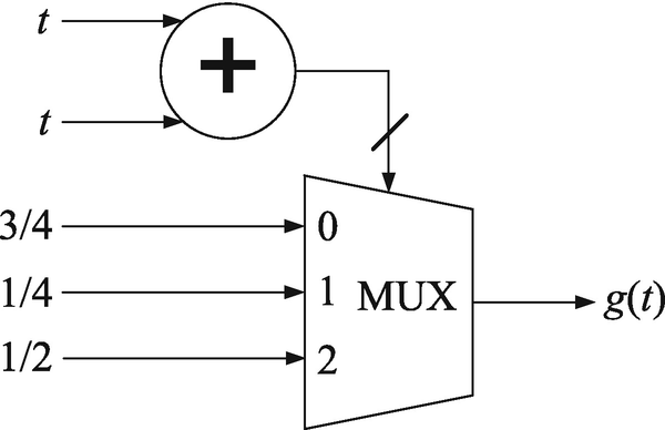

  

  A generalized multiplexing circuit implementing the polynomial $g(t) = \frac {3}{4} - t + \frac {3}{4} t^2$

Bernstein Polynomials

In this section, we introduce a specific type of polynomial that we use, namely Bernstein polynomials [12, 13].

Definition 1

A Bernstein polynomial of degree n, denoted as B _n(t), is a polynomial expressed in the following form [15]:

$$\displaystyle \begin{aligned} \sum_{k=0}^n \beta_{k,n} b_{k,n}(t), \end{aligned} $$

(12)

where each β _k,n, k = 0, 1, …, n,¹ is a real number and

$$\displaystyle \begin{aligned} b_{k,n}(t) = \binom{n}{k} t^k (1-t)^{n-k}. \end{aligned} $$

(13)

The coefficients β _k,n are called Bernstein coefficients and the polynomials b _0,n(t), b _1,n(t), …, b _n,n(t) are called Bernstein basis polynomials of degree n. $\square$

We list some pertinent properties of Bernstein polynomials.

• 1. The positivity property:For all k = 0, 1, …, n and all t in [0, 1], we have

  $$\displaystyle \begin{aligned} b_{k,n}(t) \ge 0.\end{aligned} $$

  (14)

• 2. The partition of unity property:The binomial expansion of the left-hand side of the equality (t + (1 − t))ⁿ = 1 shows that the sum of all Bernstein basis polynomials of degree n is the constant 1, i.e.,

  $$\displaystyle \begin{aligned} \sum_{k=0}^n b_{k,n}(t)=1.\end{aligned} $$

  (15)

• 3. Converting power-form coefficients to Bernstein coefficients:The set of Bernstein basis polynomials b _0,n(t), b _1,n(t), …, b _n,n(t) forms a basis of the vector space of polynomials of real coefficients and degree no more than n [14]. Each power basis function t ^j can be uniquely expressed as a linear combination of the n + 1 Bernstein basis polynomials:

  $$\displaystyle \begin{aligned} t^j = \sum_{k = 0}^n \sigma_{jk} b_{k, n}(t),\end{aligned} $$

  (16)

  for j = 0, 1, …, n. To determine the entries of the transformation matrix σ, we write

  $$\displaystyle \begin{aligned} t^j = t^j (t + (1-t))^{n-j} \end{aligned}$$

  and perform a binomial expansion on the right hand side. This gives

  $$\displaystyle \begin{aligned} t^j = \sum_{k=j}^n \frac{\binom{k}{j}}{\binom{n}{j}} b_{k,n}(t), \end{aligned}$$

  for j = 0, 1, …, n. Therefore, we have

  $$\displaystyle \begin{aligned} \sigma_{jk} = \begin{cases} \binom{k}{j} \binom{n}{j}^{-1}, &\text{for}\,\, j \le k \\ 0, &\text{for}\,\, j > k. \end{cases} \end{aligned} $$

  (17)

  Suppose that a power-form polynomial of degree no more than n is

  $$\displaystyle \begin{aligned} g(t) = \sum_{k = 0}^n a_{k, n} t^k \end{aligned} $$

  (18)

  and the Bernstein polynomial of degree n of g is

  $$\displaystyle \begin{aligned} g(t) = \sum_{k = 0}^n \beta_{k, n} b_{k,n}(t). \end{aligned} $$

  (19)

  Substituting Eqs. (16) and (17) into Eq. (18) and comparing the Bernstein coefficients, we have

  $$\displaystyle \begin{aligned} \beta_{k,n} = \sum_{j = 0}^n a_{j,n} \sigma_{jk} = \sum_{j = 0}^k \binom{k}{j} \binom{n}{j}^{-1} a_{j,n}. \end{aligned} $$

  (20)

  Equation (20) provide a means for obtaining Bernstein coefficients from power-form coefficients.

• 4. Degree elevation:

  Based on Eq. (13), we have that for all k = 0, 1, …, m,

  $$\displaystyle \begin{aligned} \begin{aligned} &\frac{1}{\binom{m+1}{k}} b_{k,m+1}(t) + \frac{1}{\binom{m+1}{k+1}} b_{k+1,m+1}(t) \\ = &t^k (1-t)^{m+1-k} + t^{k+1} (1-t)^{m-k} \\ = &t^k (1-t)^{m-k} = \frac{1}{\binom{m}{k}} b_{k,m}(t), \end{aligned} \end{aligned}$$

  or

  $$\displaystyle \begin{aligned} \begin{aligned} b_{k,m}(t) &= \frac{\binom{m}{k}}{\binom{m+1}{k}} b_{k,m+1}(t) + \frac{\binom{m}{k}}{\binom{m+1}{k+1}} b_{k+1,m+1}(t) \\ &= \frac{m+1-k}{m+1} b_{k,m+1}(t) + \frac{k+1}{m+1} b_{k+1,m+1}(t). \end{aligned} \end{aligned} $$

  (21)

  Given a power-form polynomial g of degree n, for any m ≥ n, g can be uniquely converted into a Bernstein polynomial of degree m. Suppose that the Bernstein polynomials of degree m and degree m + 1 of g are $\displaystyle {\sum _{k=0}^{m} \beta _{k,m} b_{k,m}(t)}$ and $\displaystyle {\sum _{k=0}^{m+1} \beta _{k,m+1} b_{k,m+1}(t)}$, respectively. We have

  $$\displaystyle \begin{aligned} \sum_{k=0}^{m} \beta_{k,m} b_{k,m}(t) = \sum_{k=0}^{m+1} \beta_{k,m+1} b_{k,m+1}(t). \end{aligned} $$

  (22)

  Substituting Eq. (21) into the left-hand side of Eq. (22) and comparing the Bernstein coefficients, we have

  $$\displaystyle \begin{aligned} \beta_{k, m+1} = \begin{cases} \beta_{0,m}, &\text{for}\,\, k = 0 \\ \frac{k}{m+1} \beta_{k-1, m} + \left(1 - \frac{k}{m+1}\right) \beta_{k,m}, &\text{for}\,\, 1 \le k \le m \\ \beta_{m,m}, &\text{for}\,\, k = m+1. \end{cases} \end{aligned} $$

  (23)

  Equation (23) provides a means for obtaining the coefficients of the Bernstein polynomial of degree m + 1 of g from the coefficients of the Bernstein polynomial of degree m of g. We will call this procedure degree elevation.

Uniform Approximation and Bernstein Polynomials with Coefficients in the Unit Interval

In this section, we present two of our major mathematical findings on Bernstein polynomials. The first result pertains to uniform approximation with Bernstein polynomials. We show that, given a power-form polynomial g, we can obtain a Bernstein polynomial of degree m with coefficients that are as close as desired to the corresponding values of g evaluated at the points $0, \frac {1}{m}, \frac {2}{m}, \ldots , 1$, provided that m is sufficiently large. This result is formally stated by the following theorem.

Theorem 1

Let g be a polynomial of degree n ≥ 0. For any 𝜖 > 0, there exists a positive integer M ≥ n such that for all integers m ≥ M and k = 0, 1, …, m, we have

$$\displaystyle \begin{aligned} \left|\beta_{k,m} - g\left(\frac{k}{m}\right)\right| < \epsilon, \end{aligned}$$

where β _0,m, β _1,m, …, β _m,m satisfy $\displaystyle {g(t) = \sum _{k=0}^m \beta _{k,m} b_{k,m}(t)}$. $\square$

Please see [7] for the proof of the above theorem.

The second result pertains to a special type of Bernstein polynomials: those with coefficients that are all in the unit interval. We are interested in this type of Bernstein polynomial since we can show that it can implemented by logical computation on stochastic bit streams

Definition 2

Define U to be the set of Bernstein polynomials with coefficients that are all in the unit interval [0, 1]:

$$\displaystyle \begin{aligned} \begin{array}{rcl} U &\displaystyle =&\displaystyle \Bigg\{ p(t) \ | \ \exists \ n \ge 1, 0 \le \beta_{0, n}, \beta_{1, n}, \ldots, \beta_{n,n} \le 1, \text{ such }\ \text{that }\Bigg.\\ &\displaystyle &\displaystyle \Bigg.p(t) = \sum_{k=0}^n \beta_{k,n} b_{k,n}(t) \Bigg\}. \ \square \end{array} \end{aligned} $$

The question we are interested in is: which (power-form) polynomials can be converted into Bernstein polynomials in U?

Definition 3

Define the set V to be the set of polynomials which are either identically equal to 0 or equal to 1, or map the open interval (0, 1) into (0, 1) and the points 0 and 1 into the closed interval [0, 1], i.e.,

$$\displaystyle \begin{aligned} \begin{aligned} V = \{ p(t) \ | &\ p(t) \equiv 0\text{, or } p(t) \equiv 1, \\ &\text{or } 0 < p(t) < 1, \forall t \in (0, 1) \ \text{ and } \ 0 \le p(0), p(1) \le 1 \}. \ \square \end{aligned} \end{aligned}$$

We prove that the set U and the set V are equivalent, thus giving a clear characterization of the set U.

Theorem 2

$$\displaystyle \begin{aligned} V = U. \qquad \square \end{aligned}$$

The proof of the above theorem utilizes Theorem 1. Please see [7] for the proof.

We end this section with two examples illustrating Theorem 2. In what follows, we will refer to a Bernstein polynomial of degree n converted from a polynomial g as “the Bernstein polynomial of degree n of g”. When we say that a polynomial is of degree n, we mean that the power-form of the polynomial is of degree n.

Example 1

Consider the polynomial $g(t) = \frac {5}{8} - \frac {15}{8} t + \frac {9}{4} t^2$. It maps the open interval (0, 1) into (0, 1) with $g(0) = \frac {5}{8}$ and g(1) = 1. Thus, g is in the set V . Based on Theorem 2, we have that g is in the set U. We verify this by considering Bernstein polynomials of increasing degree.

• The Bernstein polynomial of degree 2 of g is

  $$\displaystyle \begin{aligned} g(t) = \frac{5}{8} \cdot b_{0,2} (t) + \left(-\frac{5}{16}\right) \cdot b_{1, 2}(t) + 1 \cdot b_{2, 2}(t). \end{aligned}$$

  Note that the coefficient $\beta _{1,2} =- \frac {5}{16} < 0$.

• The Bernstein polynomial of degree 3 of g is

  $$\displaystyle \begin{aligned} g(t) = \frac{5}{8} \cdot b_{0,3}(t) + 0 \cdot b_{1,3}(t) + \frac{1}{8} \cdot b_{2,3}(t) + 1 \cdot b_{3,3}(t). \end{aligned}$$

  Note that all the coefficients are in [0, 1].

Since the Bernstein polynomial of degree 3 of g satisfies Definition 2, we conclude that g is in the set U. $\square$

Example 2

Consider the polynomial $g(t) = \frac {1}{4} - t + t^2$. Since g(0.5) = 0, thus g is not in the set V . Based on Theorem 2, we have that g is not in the set U. We verify this. By contraposition, suppose that there exist n ≥ 1 and 0 ≤ β _0,n, β _1,n, …, β _n,n ≤ 1 such that

$$\displaystyle \begin{aligned} g(t) = \sum_{k=0}^n \beta_{k,n} b_{k,n}(t). \end{aligned}$$

Since g(0.5) = 0, therefore, $\displaystyle {\sum _{k=0}^n \beta _{k,n} b_{k,n}(0.5) = 0}$. Note that for all k = 0, 1, …, n, b _k,n(0.5) > 0. Thus, we have that for all k = 0, 1, …, n, β _k,n = 0. Therefore, g(t) ≡ 0, which contradicts the original assumption about g. Thus, g is not in the set U. $\square$

Synthesizing Polynomial Functions

Computation on stochastic bit streams generally implements a multivariate polynomial F(x ₁, …, x _n) with integer coefficients. The degree of each variable is at most one, i.e., there are no terms with variables raised to the power of two, three or higher. If we associate some of the x _i’s of the polynomial F(x ₁, …, x _n) with real constants in the unit interval and the others with a common variable t, then the function F becomes a real-coefficient univariate polynomial g(t). With different choices of the original Boolean function f and different settings of the probabilities of the x _i’s, we get different polynomials g(t).

Example 3

Consider the function implemented by a multiplexer operating on stochastic bit streams, A, B, and S. It is a multivariate polynomial, g(a, b, s) = sa + (1 − s)b = b + sa − sb. The polynomial has integer coefficients. The degree of each variable is at most one. If we set s = a = t and b = 0.8 in the polynomial, then we get a univariate polynomial g(t) = 0.8 − 0.8t + t ². $\square$

The first question that arises is: what kind of univariate polynomials can be implemented by computation on stochastic bit streams? In [16], we proved the following theorem stating a necessary condition on the polynomials. The theorem essentially says that, given inputs that are probability values—that is to say, real values in the unit interval—the polynomial must also evaluate to a probability value. There is a caveat here: if the polynomial is not identically equal to 0 or 1, then it must evaluate to a value in the open interval (0, 1) when the input is also in the open interval (0, 1).

Theorem 3

If a polynomial g(t) can be implemented by logical computation on stochastic bit streams, then

• 1. g(t) is identically equal to 0 or 1 (g(t) ≡ 0 or 1), or

• 2. g(t) maps the open interval (0, 1) to itself (g(t) ∈ (0, 1), for all t ∈ (0, 1)) and 0 ≤ g(0), g(1) ≤ 1. $\square$

For instance, as shown in Example 3, the polynomial g(t) = 0.8 − 0.8t + t ² can be implemented by logical computation on stochastic bit streams. It is not hard to see that g(t) satisfies the necessary condition. In fact, g(0) = 0.8, g(1) = 1 and 0 < g(t) < 1, for all 0 < t < 1.

The next question that arises is: can any polynomial satisfying the necessary condition be implemented by logical computation on stochastic bit streams? If so, how? We propose a synthesis method that solves this problem; constructively, we show that, provided that a polynomial satisfies the necessary condition, we can implement it. First, in the section “Synthesizing Bernstein Polynomials with Coefficients in the Unit Interval”, we show how to implement a Bernstein polynomial with coefficients in the unit interval. Then, in the section “Synthesis of Power-Form Polynomials”, we describe how to convert a general power-form representation into such a polynomial.

Synthesizing Bernstein Polynomials with Coefficients in the Unit Interval

If all the coefficients of a Bernstein polynomial are in the unit interval, i.e., 0 ≤ b _i,n ≤ 1, for all 0 ≤ i ≤ n, then we can implement it with the construct shown in Fig. 4.

Fig. 4

Combinational logic that implements a Bernstein polynomial $B_n(t) = \sum _{i = 0}^n b_{i,n} B_{i,n}(t)$ with all coefficients in the unit interval

The block labeled “ + ” in Fig. 4 has n inputs X ₁, …, X _n and ⌈log₂(n + 1)⌉ outputs. It consists of combinational logic that computes the weight of the inputs, that is to say, it counts the number of ones in the n Boolean inputs X ₁, …, X _n, producing a binary radix encoding of this count. We will call this an n-bit Boolean “weight counter.” The multiplexer (MUX) shown in the figure has “data” inputs Z ₀, …, Z _n and the ⌈log₂(n + 1)⌉ outputs of the weight counter as the selecting inputs. If the binary radix encoding of the outputs of the weight counter is k (0 ≤ k ≤ n), then the output Y of the multiplexer is set to Z _k.

Figure 5 gives a simple design for an 8-bit Boolean weight counter based on a tree of adders. An n-bit Boolean weight counter can be implemented in a similar way.

Fig. 5

The implementation of an 8-bit Boolean weight counter

In order to implement the Bernstein polynomial

$$\displaystyle \begin{aligned} B_n(t) = \sum_{i = 0}^n b_{i,n} B_{i,n}(t),\end{aligned} $$

we set the inputs X ₁, …, X _n to be independent stochastic bit streams with probability t. Equivalently, X ₁, …, X _n can be viewed as independent random Boolean variables that have the same probability t of being one. The probability that the count of ones among the X _i’s is k (0 ≤ k ≤ n) is given by the binomial distribution:

$$\displaystyle \begin{aligned} P\left(\sum_{i=1}^n X_i = k\right) = \binom{n}{k} t^k (1-t)^{n-k} = B_{k,n}(t). \end{aligned} $$

(24)

We set the inputs Z ₀, …, Z _n to be independent stochastic bit streams with probability equal to the Bernstein coefficients b _0,n, …, b _n,n, respectively. Notice that we can represent b _i,n with stochastic bit streams because we assume that 0 ≤ b _i,n ≤ 1. Equivalently, we can view Z ₀, …, Z _n as n + 1 independent random Boolean variables that are one with probabilities b _0,n, …, b _n,n, respectively.

The probability that the output Y is one is

$$\displaystyle \begin{aligned} \begin{aligned} y &= P(Y=1) \\ &= \sum_{k = 0}^n \left(P \left(Y=1 | \sum_{i=1}^n X_i = k\right) P \left(\sum_{i=1}^n X_i = k\right) \right).\vspace{2pt} \end{aligned} \end{aligned} $$

(25)

Since the multiplexer sets Y equal to Z _k, when $\sum _{i=1}^n X_i = k$, we have

$$\displaystyle \begin{aligned} P\left(Y=1 | \sum_{i=1}^n X_i = k\right) = P(Z_k = 1) = b_{k,n}.\end{aligned} $$

(26)

Thus, from Eqs. (13), (24), (25), and (26), we have

$$\displaystyle \begin{aligned} y = \sum_{k = 0}^n b_{k,n} B_{k,n}(t) = B_n(t).\end{aligned} $$

(27)

We conclude that the circuit in Fig. 4 implements the given Bernstein polynomial with all coefficients in the unit interval. We have the following theorem.

Theorem 4

If all the coefficients of a Bernstein polynomial are in the unit interval, i.e., 0 ≤ b _i,n ≤ 1, for 0 ≤ i ≤ n, then we can synthesize logical computation on stochastic bit streams to implement it. $\square$

Example 4

The polynomial $\displaystyle {g_1(t) = \frac {1}{4} + \frac {9}{8} t - \frac {15}{8} t^2 + \frac {5}{4} t^3}$ can be converted into a Bernstein polynomial of degree 3:

$$\displaystyle \begin{aligned} g_1(t) = \frac{2}{8} B_{0,3}(t) + \frac{5}{8} B_{1,3}(t) + \frac{3}{8} B_{2,3}(t) + \frac{6}{8} B_{3,3}(t). \qquad \square\end{aligned} $$

Figure 6 shows a circuit that implements this Bernstein polynomial. The function is evaluated at t = 0.5. The stochastic bit streams X ₁, X ₂ and X ₃ are independent, each with probability t = 0.5. The stochastic bit streams Z ₀, …, Z ₃ have probabilities $\frac {2}{8}$, $\frac {5}{8}$, $\frac {3}{8}$, and $\frac {6}{8}$, respectively. As expected, the computation produces the correct output value: g ₁(0.5) = 0.5. $\square$

Fig. 6

Computation on stochastic bit streams that implements the Bernstein polynomial $g_1(t) = \frac {2}{8} B_{0,3}(t) + \frac {5}{8} B_{1,3}(t) + \frac {3}{8} B_{2,3}(t) + \frac {6}{8} B_{3,3}(t)$ at t = 0.5

Synthesis of Power-Form Polynomials

In the previous section, we saw that we can implement a polynomial through logical computation on stochastic bit streams if the polynomial can be represented as a Bernstein polynomial with coefficients in the unit interval. A question that arises is: what kind of polynomials can be represented in this form? Generally, we seek to implement polynomials given to us in power form. In [16], we proved that any polynomial that satisfies Theorem 3—so essentially any polynomial that maps the unit interval onto the unit interval—can be converted into a Bernstein polynomial with all coefficients in the unit interval.² Based on this result and Theorem 4, we can see that the necessary condition shown in Theorem 3 is also a sufficient condition for a polynomial to be implemented by logical computation on stochastic bit streams.

Example 5

Consider the polynomial g ₂(t) = 3t − 8t ² + 6t ³ of degree 3, Since g ₂(t) ∈ (0, 1), for all t ∈ (0, 1) and g ₂(0) = 0, g ₂(1) = 1, it satisfies the necessary condition shown in Theorem 3. Note that

$$\displaystyle \begin{aligned} \begin{aligned} g_2(t) &= B_{1,3}(t) - \frac{2}{3} B_{2,3}(t) + B_{3,3}(t) \\ &= \frac{3}{4} B_{1,4}(t) + \frac{1}{6} B_{2,4}(t) - \frac{1}{4} B_{3,4}(t) + B_{4,4}(t) \\ &= \frac{3}{5} B_{1,5}(t) + \frac{2}{5} B_{2,5}(t) + B_{5,5}(t). \end{aligned} \end{aligned}$$

Thus, the polynomial g ₂(t) can be converted into a Bernstein polynomial with coefficients in the unit interval. The degree of such a Bernstein polynomial is 5, greater than that of the original power form polynomial. $\square$

Given a power-form polynomial $g(t) = \sum _{i=0}^{n} a_{i,n} t^i$ that satisfies the condition of Theorem 3, we can synthesize it in the following steps:

• 1. Let m = n. Obtain b _0,m, b _1,m, …, b _m,m from a _0,n, a _1,n, …, a _n,n by Eq. (16).

• 2. Check to see if 0 ≤ b _i,m ≤ 1, for all i = 0, 1, …, m. If so, go to step 4.

• 3. Let m = m + 1. Calculate b _0,m, b _1,m, …, b _m,m from b _0,m−1, b _1,m−1, …, b _m−1,m−1 based on Eq. (13). Go to step 2.

• 4. Synthesize the Bernstein polynomial

  $$\displaystyle \begin{aligned} B_m(t) = \sum_{i=0}^m b_{i,m} B_{i,m}(t) \end{aligned}$$

  with the generalized multiplexing construct in Fig. 4.

Synthesizing Non-Polynomial Functions

In real applications, we often encounter non-polynomial functions, such as trigonometric functions. In this section, we discuss the implementation of such functions; further details are given in [18]. Our strategy is to approximate them by Bernstein polynomials with coefficients in the unit interval. In the previous section, we saw how to implement such Bernstein polynomials.

We formulate the problem of implementing an arbitrary function g(t) as follows. Given g(t), a continuous function on the unit interval, and n, the degree of a Bernstein polynomial, find real numbers b _i,n, i = 0, …, n, that minimize

$$\displaystyle \begin{aligned} \int_0^1 (g(t) - \sum_{i=0}^n b_{i,n} B_{i,n}(t))^2 \,\mathrm{d} t, \end{aligned} $$

(28)

subject to

$$\displaystyle \begin{aligned} 0 \le b_{i,n} \le 1, \text{for all}\,\, i =0, 1, \ldots, n. \end{aligned} $$

(29)

Here we try to find the optimal approximation by minimizing an objective function, Eq. (28), that measures the approximation error. This is the square of the L ² norm on the difference between the original function g(t) and the Bernstein polynomial $B_n(t) = \sum _{i=0}^n b_{i,n} B_{i,n}(t)$. The integral is on the unit interval because t, representing a probability value, is always in the unit interval. The constraints in Eq. (29) guarantee that the Bernstein coefficients are all in the unit interval. With such coefficients, the construct in Fig. 4 computes an optimal approximation of the function.

The optimization problem is a constrained quadratic programming problem [18]. Its solution can be obtained using standard techniques.

Example 6

Consider the non-polynomial function g ₃(t) = t ^0.45. We approximate this function by a Bernstein polynomial of degree 6. By solving the constrained quadratic optimization problem, we obtain the Bernstein coefficients:

$$\displaystyle \begin{aligned} &b_{0,6} = 0.0955, b_{1,6} = 0.7207, b_{2,6} = 0.3476, b_{3,6} = 0.9988, \\ &b_{4,6} = 0.7017, b_{5,6} = 0.9695, b_{6,6} = 0.9939. \qquad \square \end{aligned} $$

Discussion

This chapter presented a necessary and sufficient condition for synthesizing stochastic functions with combinational logic: the target function must be a polynomial that maps the unit interval [0, 1] to the unit interval [0, 1]. The “necessary” part was easy: given stochastic inputs, any combinational circuits produces a polynomial. Since the inputs and outputs are probabilities, this polynomial maps the unit interval to the unit interval.

The “sufficient” part entailed some mathematics. First we showed that any polynomial given in power form can be transformed into a Bernstein polynomial. This was well known [13]. Next we showed that, by elevating the degree of the Bernstein polynomial, we always obtain a Bernstein polynomial with coefficients in the unit interval. This was a new result, published in [16]. Finally, we showed that any Bernstein polynomial with coefficients in the unit interval can be implemented by a form of “general multiplexing”. These results were published in [17, 18].

The synthesis method is both general and efficient. For a wide variety of applications, it produces stochatic circuits that have remarkably small area, compared to circuits that operate on a conventional binary positional encodings [18]. We note that our characterization applies only to combinational circuits, that is to say logic circuits without memory elements. Dating back to very interesting work by Brown & Card [4], researchers have explored stochastic computing with sequential circuits, that is to say logic circuits with memory elements. With sequential circuits, one can implement a much larger class of functions than polynomials. For instance, Brown & Card showed that a sequential circuit can implement the tanh function. A complete characterization of what sort of stochastic functions can be computed by sequential circuits has not been established. However, we point the reader to recent work on the topic: [19,20,21,22].

References

B. Gaines, “Stochastic computing systems,” in Advances in Information Systems Science. Plenum Press, 1969, vol. 2, ch. 2, pp. 37–172.
W. J. Poppelbaum, A. Dollas, J. B. Glickman, and C. Otoole, “Statistical processors,” in Advances in Computers, M. C. Yovits, Ed., 1976, vol. 17, pp. 187–230.
——, “Unary processing,” in Advances in Computers, M. C. Yovits, Ed., 1987, vol. 26, pp. 48–89.
B. Brown and H. Card, “Stochastic neural computation I: Computational elements,” IEEE Transactions on Computers, vol. 50, no. 9, pp. 891–905, 2001.
P. Li, D. J. Lilja, W. Qian, K. Bazargan, and M. D. Riedel, “Computation on stochastic bit streams: Digital image processing case studies,” IEEE Transactions on VLSI Systems, vol. 22, pp. 449–462, 2014.
A. Ardakani, F. Leduc-Primeau, N. Onizawa, T. Hanyu, and W. J. Gross, “Vlsi implementation of deep neural network using integral stochastic computing,” IEEE Transactions on Very Large Scale Integration (VLSI) Systems, vol. 25, no. 10, pp. 2688–2699, Oct 2017.
W. Qian, “Digital yet deliberately random: Synthesizing logical computation on stochastic bit streams,” Ph.D. dissertation, University of Minnesota, 2011.
K. P. Parker and E. J. McCluskey, “Probabilistic treatment of general combinational networks,” IEEE Transactions on Computers, vol. 24, no. 6, pp. 668–670, 1975.
J. Savir, G. Ditlow, and P. H. Bardell, “Random pattern testability,” IEEE Transactions on Computers, vol. 33, no. 1, pp. 79–90, 1984.
J.-J. Liou, K.-T. Cheng, S. Kundu, and A. Krstic, “Fast statistical timing analysis by probabilistic event propagation,” in Design Automation Conference, 2001, pp. 661–666.
R. Marculescu, D. Marculescu, and M. Pedram, “Logic level power estimation considering spatiotemporal correlations,” in International Conference on Computer-Aided Design, 1994, pp. 294–299.
S. N. Bernstein, “Démonstration du théorème de Weierstrass fondée sur le calcul des probabilités,” Communications of the Kharkov Mathematical Society, vol. 13, pp. 1–2, 1912.
G. Lorentz, Bernstein Polynomials. University of Toronto Press, 1953.
R. Farouki and V. Rajan, “On the numerical condition of polynomials in Bernstein form,” Computer Aided Geometric Design, vol. 4, no. 3, pp. 191–216, 1987.
J. Berchtold and A. Bowyer, “Robust arithmetic for multivariate Bernstein-form polynomials,” Computer-Aided Design, vol. 32, no. 11, pp. 681–689, 2000.
W. Qian, M. D. Riedel, and I. Rosenberg, “Uniform approximation and Bernstein polynomials with coefficients in the unit interval,” European Journal of Combinatorics, vol. 32, no. 3, pp. 448–463, 2011.
W. Qian and M. D. Riedel, “The synthesis of robust polynomial arithmetic with stochastic logic,” in Design Automation Conference, 2008, pp. 648–653.
W. Qian, X. Li, M. D. Riedel, K. Bazargan, and D. J. Lilja, “An architecture for fault-tolerant computation with stochastic logic,” IEEE Transactions on Computers, vol. 60, no. 1, pp. 93–105, 2011.
P. Li, W. Q. M. D. Riedel, K. Bazargan, and D. J. Lilja, “The synthesis of linear finite state machine-based stochastic computational elements,” in Asia and South Pacific Design Automation Conference, 2012, pp. 757–762.
P. Li, D. Lilja, W. Qian, K. Bazaragan, and M. D. Riedel, “The synthesis of complex arithmetic computation on stochastic bit streams using sequential logic,” in International Conference on Computer-Aided Design, 2012, pp. 480–487.
P. Li, D. J. Lilja, W. Qian, M. D. Riedel, and K. Bazargan, “Logical computation on stochastic bit streams with linear finite state machines,” IEEE Transactions on Computers, 2013.
N. Saraf and K. Bazargan, “Sequential logic to transform probabilities,” in International Conference on Computer-Aided Design, 2013.
Author information
Authors and Affiliations
Corresponding author
Editor information
Editors and Affiliations
Rights and permissions
Copyright information
© 2019 Springer Nature Switzerland AG
About this chapter
Cite this chapter
Riedel, M., Qian, W. (2019). Synthesis of Polynomial Functions. In: Gross, W., Gaudet, V. (eds) Stochastic Computing: Techniques and Applications. Springer, Cham. https://doi.org/10.1007/978-3-030-03730-7_5
Download citation
DOI: https://doi.org/10.1007/978-3-030-03730-7_5
Published:
Publisher Name: Springer, Cham
Print ISBN: 978-3-030-03729-1
Online ISBN: 978-3-030-03730-7
eBook Packages: EngineeringEngineering (R0)