Geometric Flow Equations

Abstract

In this minicourse, we study hypersurfaces that solve geometric evolution equations. More precisely, we investigate hypersurfaces that evolve with a normal velocity depending on a curvature function like the mean curvature or Gauß curvature. In three lectures, we address

• hypersurfaces, principal curvatures and evolution equations for geometric quantities like the metric and the second fundamental form.

• the convergence of convex hypersurfaces to round points. Here, we will also show some computer algebra calculations.

• the evolution of graphical hypersurfaces under mean curvature flow.

1 Overview and Plan for the Summer School

We consider flow equations that deform hypersurfaces according to their curvature.

If $X_0:M^n\to {\mathbb {R}}^{n+1}$ is an embedding of an n-dimensional manifold, we can define principal curvatures (λ _i)_1≤i≤n and a normal vector ν. We deform the embedding vector X according to

$$\displaystyle \begin{aligned}\begin{cases} {\frac{d}{dt}} X=-F\nu,&\\ X(\cdot,0)=X_0,& \end{cases}\end{aligned} $$

where F is a symmetric function of the principal curvatures, e.g. the mean curvature H = λ ₁ + ⋯ + λ _n. In this way, we obtain a family X(⋅, t) of embeddings and study their behaviour especially near singularities and for large times. We consider hypersurfaces that contract to a point in finite time and, after appropriate rescaling, to a round sphere. Graphical solutions are shown to exist for all times or to disappear to infinity.

Classical results in this direction were obtained by Huisken [20] and Ecker and Huisken [11] for mean curvature flow.

Remark 1

• (i) We will use geometric flow equations as a tool to deform a manifold.

• (ii) The flow equations considered are parabolic equations like the heat equation.

• (iii) In order to control the behaviour of the flow, we will look for properties of the manifold that are preserved under the flow. For that purpose, we will also look for quantities that are monotone and have geometric significance, i.e. their boundedness implies geometric properties of the evolving manifold.

We wish to thank Ben Lambert and Wolfgang Maurer for corrections and Wolfgang Maurer for carefully preparing the figures.

1.1 Plan for the Summer School

These notes first cover some necessary background material. We will then derive evolution equations for geometric quantities and study two geometric problems. More precisely, our plan is to study the following:

• Geometric prerequisites and evolution equations of geometric quantities.

• Convex surfaces contracting to a round point and an estimate for Gauß curvature flow, Theorem 6, measuring the deviation from being umbilic.

• Mean curvature flow of complete graphs and local C ¹-bounds, Theorem 16.

2 Differential Geometry of Submanifolds

We will only consider hypersurfaces in Euclidean space.

We use $X=X(x,\,t)=\left (X^\alpha \right )_{1\le \alpha \le n+1}$ to denote the time-dependent embedding vector of a manifold M ⁿ into ${\mathbb {R}}^{n+1}$ and ${\frac {d}{dt}} X=\dot X$ for its total time derivative. Set $M_t:=X(M,\,t)\subset {\mathbb {R}}^{n+1}$. We will often identify an embedded manifold with its image. We will assume that X is smooth. Assume furthermore that M ⁿ is smooth, orientable, connected, complete and ∂M ⁿ = ∅. We choose $\nu =\nu (x)=\left (\nu ^\alpha \right )_{1\le \alpha \le n+1}$ to be the outer (or downward pointing) unit normal vector to M _t at x ∈ M _t. The embedding X(⋅, t) induces at each point on M _t a metric (g _ij)_1≤i,j≤n and a second fundamental form (h _ij)_1≤i,j≤n. Let (g ^ij) denote the inverse of (g _ij). These tensors are symmetric. The principal curvatures (λ _i)_1≤i≤n are the eigenvalues of the second fundamental form with respect to that metric. That is, at p ∈ M, for each principal curvature λ _i, there exists $0\neq \xi \in T_pM\cong {\mathbb {R}}^n$ such that

$$\displaystyle \begin{aligned}\lambda_i\sum\limits_{l=1}^n g_{kl}\xi^l=\sum\limits_{l=1}^n h_{kl}\xi^l\quad \text{or, equivalently,}\quad \lambda_i\xi^l=\sum\limits_{k,r=1}^n g^{lk}h_{kr}\xi^r.\end{aligned}$$

As usual, eigenvalues are listed according to their multiplicity. A hypersurface is called strictly convex, if all principal curvatures are strictly positive. The inverse of the second fundamental form is denoted by $\big (\tilde h^{ij}\big )_{1\le i,\,j\le n}$.

Latin indices range from 1 to n and refer to geometric quantities on the hypersurface, Greek indices range from 1 to n + 1 and refer to components in the ambient space ${\mathbb {R}}^{n+1}$. In ${\mathbb {R}}^{n+1}$, we will always choose Euclidean coordinates. We use the Einstein summation convention for repeated upper and lower indices. Latin indices are raised and lowered with respect to the induced metric or its inverse $\left (g^{ij}\right )$, for Greek indices we use the flat metric $(\overline g_{\alpha \beta })_{1\le \alpha ,\beta \le n+1} =(\delta _{\alpha \beta })_{1\le \alpha ,\beta \le n+1}$ of ${\mathbb {R}}^{n+1}$. So the defining equation for the principal curvatures becomes λ _i g _kl ξ ^l = h _kl ξ ^l.

Denoting by 〈⋅, ⋅〉 the Euclidean scalar product in ${\mathbb {R}}^{n+1}$, we have

$$\displaystyle \begin{aligned}g_{ij}=\left\langle X_{,\,i},\,X_{,\,j}\right\rangle =X^\alpha_{,\,i}\delta_{\alpha\beta}X^\beta_{,\,j}\,,\end{aligned}$$

where we used indices, preceded by commas, to denote partial derivatives. We write indices, preceded by semi-colons, e.g. h _{ij; k} or v _;k, to indicate covariant differentiation with respect to the induced metric. Later, we will also drop the commas and semi-colons, if the meaning is clear from the context. We set $X^\alpha _{;i}\equiv X^\alpha _{,i}$ and

$$\displaystyle \begin{aligned} X^\alpha_{;\,ij}=X^\alpha_{,\,ij}-\varGamma^k_{ij}X^\alpha_{,\,k}, \end{aligned} $$

(1)

where

$$\displaystyle \begin{aligned}\varGamma^k_{ij}=\tfrac12g^{kl}(g_{il,\,j}+g_{jl,\,i}-g_{ij,\,l})\end{aligned}$$

are the Christoffel symbols of the metric (g _ij). Therefore, $X^\alpha _{;ij}$ becomes a tensor.

The Gauß formula relates covariant derivatives of the position vector to the second fundamental form and the normal vector

$$\displaystyle \begin{aligned} X^\alpha_{;\,ij}=-h_{ij}\nu^\alpha. \end{aligned} $$

(2)

The Weingarten equation allows to compute derivatives of the normal vector

$$\displaystyle \begin{aligned} \nu^\alpha_{;\,i}=h^k_iX^\alpha_{;\,k}. \end{aligned} $$

(3)

We can use the Gauß formula (2) or the Weingarten equation (3) to compute the second fundamental form.

Symmetric functions of the principal curvatures are well-defined, we will use the mean curvature H = λ ₁ + … + λ _n, the square of the norm of the second fundamental form $|A|{ }^2=\lambda _1^2+\ldots +\lambda _n^2$, $\operatorname {\mathrm {tr}} A^k= \lambda _1^k +\ldots +\lambda _n^k$, and the Gauß curvature K = λ ₁ ⋅… ⋅ λ _n. It is often convenient to choose coordinate systems such that, at a fixed point, the metric tensor equals the Kronecker delta, g _ij = δ _ij, and (h _ij) is diagonal, $(h_{ij})= \operatorname {\mathrm {diag}}(\lambda _1,\ldots ,\lambda _n)$, e.g.

$$\displaystyle \begin{aligned}\sum\lambda_k h_{ij;k}^2=\sum_{i,\,j,\,k=1}^n \lambda_k h_{ij;k}^2 =h^{kl}h^i_{j;\,k}h^j_{i;\,l} =h_{rs}h_{ij;\,k}h_{ab;\,l}g^{ia}g^{jb}g^{rk}g^{sl}.\end{aligned}$$

Whenever we use this notation, we will also assume that we have fixed such a coordinate system.

A normal velocity F can be considered as a function of (λ ₁, …, λ _n) or (h _ij, g _ij). If F(λ _i) is symmetric and smooth, then F(h _ij, g _ij) is also smooth [17, Theorem 2.1.20]. We set $F^{ij}={\frac {\partial F}{\partial h_{ij}}}$, $F^{ij,\,kl}={\frac {\partial ^2F}{\partial h_{ij}\partial h_{kl}}}$. Note that in coordinate systems with diagonal h _ij and g _ij = δ _ij as mentioned above, F ^ij is diagonal. For F = |A|², we have F ^ij = 2h ^ij = 2λ _i g ^ij, and for F = K ^α, α > 0, we have $F^{ij}=\alpha K^{\alpha }\tilde h^{ij}= \alpha K^{\alpha }\lambda _i^{-1}g^{ij}$.

The Gauß equation expresses the Riemannian curvature tensor of the hypersurface in terms of the second fundamental form

$$\displaystyle \begin{aligned} R_{ijkl}=h_{ik}h_{jl}-h_{il}h_{jk}. \end{aligned} $$

(4)

As we use only Euclidean coordinate systems in ${\mathbb {R}}^{n+1}$, h _{ij; k} is symmetric in all three indices according to the Codazzi equations.

The Ricci identity allows to interchange covariant derivatives. We will use it for the second fundamental form

$$\displaystyle \begin{aligned} h_{ik;\,lj}=h_{ik;\,jl}+h^a_kR_{ailj}+h^a_iR_{aklj}. \end{aligned} $$

(5)

For tensors A and B, A _ij ≥ B _ij means that (A _ij − B _ij) is positive semi-definite.

Finally, we use c to denote universal, estimated constants.

2.1 Graphical Submanifolds

Lemma 1

Let $u:{\mathbb {R}}^n\to {\mathbb {R}}$ be smooth. Then $\operatorname {\mathrm {graph}} u$ is a submanifold in ${\mathbb {R}}^{n+1}$ . The metric g _ij , the lower unit normal vector ν, the second fundamental form h _ij , the mean curvature H, and the Gauß curvature K are given by

$$\displaystyle \begin{aligned} g_{ij}=&\,\delta_{ij}+u_iu_j,\\ g^{ij}=&\,\delta^{ij}-\frac{u^iu^j}{1+|Du|{}^2},\\ \nu=&\,\frac{((u_i),-1)}{\sqrt{1+|Du|{}^2}}\equiv\frac{((u_i),-1)} {\mathrm{v}},\\ h_{ij}=&\,\frac{u_{ij}}{\sqrt{1+|Du|{}^2}}\equiv \frac{u_{ij}}{\mathrm{v}},\\ H=&\,\operatorname{\mathrm{div}}\left(\frac{Du}{\sqrt{1+|Du|{}^2}}\right), \end{aligned} $$

and

$$\displaystyle \begin{aligned} K=&\,\frac{\det D^2u}{\left(1+|Du|{}^2\right)^{\frac{n+2}2}}, \end{aligned} $$

where $u_i\equiv {\frac {\partial u}{\partial x^i}}$ , u ⁱ = u _j δ ^ji and $u_{ij}={\frac {\partial ^2u}{\partial x^i\partial x^j}}$ . Note that in Euclidean space, we often do not distinguish between Du and ∇u.

Proof

• (i) We use the embedding vector X(x) := (x, u(x)), $X:{\mathbb {R}}^n\to {\mathbb {R}}^{n+1}$. The induced metric is the pull-back of the Euclidean metric in ${\mathbb {R}}^{n+1}$, $g:=X^*g_{{\mathbb {R}}^{n+1}_{\text{Eucl.}}}$. We have X _,i = (e _i, u _i). Hence

  $$\displaystyle \begin{aligned}g_{ij}=X_{,i}^\alpha\delta_{\alpha\beta}X^\beta_{,j} =\langle X_{,i},X_{,j}\rangle =\langle(e_i,u_i),(e_j,u_j)\rangle =\delta_{ij}+u_iu_j.\end{aligned}$$

• (ii) It is easy to check, that g ^ij is the inverse of g _ij. Note that u ⁱ := δ ^ij u _j, i.e., we lift the index with respect to the flat metric.

• (iii) The vectors X _,i = (e _i, u _i) are tangent to $\operatorname {\mathrm {graph}} u$. The vector ((−u _i), 1) ≡ (−Du, 1) is orthogonal to these vectors, hence, up to normalization, a unit normal vector.

• (iv) We combine (1), (2) and compute the scalar product with ν to get

  $$\displaystyle \begin{aligned} h_{ij} =&\,-\langle X_{;ij},\nu\rangle =-\langle X_{,ij}-\varGamma^k_{ij}X_{,k},\nu\rangle =-\langle X_{,ij},\nu\rangle\\ =&\,-\left\langle(0,u_{ij}), \frac{((u_i),-1)}{\mathrm{v}}\right\rangle =\frac{u_{ij}}{\mathrm{v}}. \end{aligned} $$

• (v) We obtain

  $$\displaystyle \begin{aligned} H =&\,\sum_{i=1}^n\lambda_i=g^{ij}h_{ij} =\left(\delta^{ij}-\frac{u^iu^j}{1+|Du|{}^2}\right) \frac{u_{ij}}{\sqrt{1+|Du|{}^2}}\\ =&\,\frac{\delta^{ij}u_{ij}}{\sqrt{1+|Du|{}^2}} -\frac{u^iu^ju_{ij}}{\left(1+|Du|{}^2\right)^{3/2}}\\ =&\,\frac{\varDelta u}{\sqrt{1+|Du|{}^2}} -\frac{u^iu^ju_{ij}}{\left(1+|Du|{}^2\right)^{3/2}} \end{aligned} $$

  and, on the other hand,

  $$\displaystyle \begin{aligned} \operatorname{\mathrm{div}}\left(\frac{Du}{\sqrt{1+|Du|{}^2}}\right) =&\,\sum_{i=1}^n{\frac{\partial }{\partial x^i}}\frac{u_i}{\sqrt{1+|Du|{}^2}}\\ =&\,\sum_{i=1}^n\frac{u_{ii}}{\sqrt{1+|Du|{}^2}} -\sum_{i,j=1}^n \frac{u_iu_ju_{ji}}{\left(1+|Du|{}^2\right)^{3/2}}\\ =&\,H. \end{aligned} $$

• (vi) From the defining equation for the principal curvatures and $\det g_{ij}=1+|Du|{ }^2$, we obtain

  $$\displaystyle \begin{aligned} K=&\,\prod_{i=1}^n\lambda_i =\det\,\left(g^{ij}h_{jk}\right) =\det g^{ij}\cdot\det h_{ij} =\frac{\det h_{ij}}{\det g_{ij}}\\ =&\,\frac{\mathrm{v}^{-n}\det u_{ij}}{\mathrm{v}^2} =\frac{\det D^2u}{\left(1+|Du|{}^2\right)^{\frac{n+2}2}}. \end{aligned} $$

□

These formulae extend to the situation, in which u is defined on an open subset of ${\mathbb {R}}^n$.

Exercise 1 (Spheres)

The lower hemisphere of radius R is locally given as $\operatorname {\mathrm {graph}} u$ with $u:B_R(0)\to {\mathbb {R}}$ defined by $u(x):=-\sqrt {R^2-|x|{ }^2}$. Compute all the quantities mentioned in Lemma 1 and the principal curvatures explicitly for this example.

Exercise 2

Give a geometric definition of the (principal) curvature of a curve in ${\mathbb {R}}^2$ in terms of a circle approximating that curve in an optimal way.

Use the min-max characterization of eigenvalues to extend that geometric definition to n-dimensional hypersurfaces in ${\mathbb {R}}^{n+1}$.

Exercise 3 (Rotationally Symmetric Graphs)

Assume that the function $u:{\mathbb {R}}^n\to {\mathbb {R}}$ is smooth and u(x) = u(y), if |x| = |y|. Then u(x) = f(|x|) for some $f:{\mathbb {R}}_+\to {\mathbb {R}}$. Compute once again all the geometric quantities mentioned in Lemma 1.

3 Evolving Submanifolds

3.1 General Assumption

We will only consider the evolution of manifolds of dimension n embedded into ${\mathbb {R}}^{n+1}$, i.e. the evolution of hypersurfaces in Euclidean space. (Mean curvature flow is also considered for manifolds of arbitrary codimension. Another generalisation is to study flow equations of hypersurfaces immersed into Riemannian or Lorentzian manifolds.)

Definition 1

Let M ⁿ denote an orientable manifold of dimension n. Let $X(\cdot ,t):M^n\to {\mathbb {R}}^{n+1}$, 0 ≤ t ≤ T < ∞, be a smooth family of smooth embeddings. Let ν denote one choice of the normal vector field along X(M ⁿ, t). Then X or (M _t)_0≤t<T with M _t := X(M ⁿ, t) is said to move with normal velocity F, if

$$\displaystyle \begin{aligned}{\frac{d}{dt}} X=-F\nu\quad \text{in }M^n\times[0,T).\end{aligned}$$

Remark 2

In codimension 1, we often do not need to assume that M ⁿ is orientable: Let X : M ⁿ → N ⁿ⁺¹ be a C ²-immersion and $H_1(N;{\mathbb {Z}}/2{\mathbb {Z}})=0$. Assume that X is proper, X ⁻¹(∂N) = ∂M, and X is transverse to ∂N. Then N ∖ X(M) is not connected [13]. Hence, if M ⁿ is closed and embedded in ${\mathbb {R}}^{n+1}$, M ⁿ is orientable.

3.2 Evolution of Graphs

Lemma 2

Let $u:{\mathbb {R}}^n\times [0,\infty )\to {\mathbb {R}}$ be a smooth function such that $\operatorname {\mathrm {graph}} u$ evolves according to ${\frac {d}{dt}} X=-F\nu$ . Then

$$\displaystyle \begin{aligned}\dot u=\sqrt{1+|Du|{}^2}\cdot F.\end{aligned}$$

This result also holds, if u is defined on an open subset of ${\mathbb {R}}^n\times [0,\infty )$.

Proof

Beware of assuming that the (n + 1)-st component in the evolution equation ${\frac {d}{dt}} X=-F\nu$ were equal to $\dot u$ as a hypersurface evolving according to ${\frac {d}{dt}} X=-F\nu$ does not only move in vertical direction but also in horizontal direction.

Let p denote a point on the abstract manifold embedded via X into ${\mathbb {R}}^{n+1}$. As our embeddings are graphical, we see that

$$\displaystyle \begin{aligned}X(p,t)=(x(p,t),u(x(p,t),t)).\end{aligned}$$

We consider the scalar product of both sides of the evolution equation with ν and obtain

$$\displaystyle \begin{aligned}F=\langle F\nu,\nu\rangle=\left\langle-{\frac{d}{dt}} X,\nu\right\rangle =-\left\langle\left(\left(\dot x^k\right),u_i\dot x^i+\dot u\right),\frac{((u_i),-1)}{\sqrt{1+|Du|{}^2}}\right\rangle =\frac{\dot u}{\sqrt{1+|Du|{}^2}}.\end{aligned}$$

□

Corollary 1

Let $u:{\mathbb {R}}^n\times [0,\infty )\to {\mathbb {R}}$ be a smooth function such that $\operatorname {\mathrm {graph}} u$ solves mean curvature flow ${\frac {d}{dt}} X=-H\nu$ . Then

$$\displaystyle \begin{aligned}\dot u=\sqrt{1+|Du|{}^2}\cdot \operatorname{\mathrm{div}}\left(\frac{Du}{\sqrt{1+|Du|{}^2}}\right).\end{aligned}$$

Exercise 4 (Rotationally Symmetric Translating Solutions)

Let $u:={\mathbb {R}}^n\times {\mathbb {R}}\to {\mathbb {R}}$ be rotationally symmetric. Assume that $\operatorname {\mathrm {graph}} u$ is a translating solution to mean curvature flow ${\frac {d}{dt}} X=-H\nu$, i.e. a solution such that $\dot u$ is constant.

Similar to Exercise 3, derive an ordinary differential equation for translating rotationally symmetric solutions to mean curvature flow.

Why does it suffice to consider the case $\dot u=1$?

Remark 3

Consider a physical system consisting of a domain $\varOmega \subset {\mathbb {R}}^3$. Assume that the energy of the system is proportional to the surface area of ∂Ω. Then, up to a transformation t↦μt for some μ > 0, the L ²-gradient flow for the area is mean curvature flow. We check that in a model case for graphical solutions in Lemma 3.

Lemma 3

Let $u:{\mathbb {R}}^n\times [0,\infty )\to {\mathbb {R}}$ be smooth. Assume that u(x, t) ≡ 0 for |x|≥ R. Then the surface area is maximally reduced among all normal velocities F with given L ² -norm, if the normal velocity of $\operatorname {\mathrm {graph}} u$ is given by H, i.e. if $\dot u=\sqrt {1+|Du|{ }^2}\cdot H$.

Note that in general, soluIons to $\dot u = \sqrt {1+|Du|{ }^2}\cdot H$ do not have compact support.

Proof

The area of $\operatorname {\mathrm {graph}} u(\cdot ,t)|{ }_{B_R}$ is given by

$$\displaystyle \begin{aligned}A(t)=\int\limits_{B_R}\sqrt{1+|Du|{}^2}\,dx.\end{aligned}$$

Define the induced area element dμ by $d\mu :=\sqrt {1+|Du|{ }^2}\,dx$. We obtain using integration by parts

$$\displaystyle \begin{aligned} \left.{\frac{d}{dt}} A(t)\right|{}_{t=0}=&\,\left.\int\limits_{B_R}{\frac{d}{dt}} \sqrt{1+|Du|{}^2}\,dx\,\right|{}_{t=0} =\left.\int\limits_{B_R(0)}\frac{1}{\sqrt{1+|Du|{}^2}} \langle Du,D\dot u\rangle\,\right|{}_{t=0}\\ =&\,-\left.\int\limits_{B_R} \operatorname{\mathrm{div}}\left(\frac{Du} {\sqrt{1+|Du|{}^2}}\right)\frac{\dot u}{\mathrm{v}}\cdot \mathrm{v}\,dx\,\right|{}_{t=0} =-\left.\int\limits_{B_R}H\,F\,d\mu\,\right|{}_{t=0}\\ \ge&\,-\left.\left(\;\int\limits_{B_R}H^2\,d\mu\right)^{1/2} \left(\;\int\limits_{B_R}F^2\,d\mu\right)^{1/2}\right|{}_{t=0}. \end{aligned} $$

Here, we have used Hölder’s inequality $\|ab\|{ }_{L^1} \le \|a\|{ }_{L^2} \cdot \|b\|{ }_{L^2}$. There, we get equality precisely if a and b differ only by a multiplicative constant. Hence the surface area is reduced most efficiently among all normal velocities F with $\|F\|{ }_{L^2}=\|H\|{ }_{L^2}$, if we choose F = H. In this sense, mean curvature flow is the L ²-gradient flow for the area integral. □

3.3 Examples

Lemma 4

Consider mean curvature flow, i.e. the evolution equation ${\frac {d}{dt}} X=-H\nu$ , with M ₀ = ∂B _R(0). Then a smooth solution exists for $0\le t<T:=\frac {1}{2n}R^2$ and is given by M _t = ∂B _r(t)(0) with $r(t)=\sqrt {2n(T-t)}=\sqrt {R^2-2nt}$.

Proof

The mean curvature of a sphere of radius r(t) is given by $H=\frac n{r(t)}$. Hence we obtain a solution to mean curvature flow, if r(t) fulfills

$$\displaystyle \begin{aligned}\dot r(t)=\frac{-n}{r(t)}.\end{aligned}$$

A solution to this ordinary differential equation is given by $r(t)=\sqrt {2n(T-t)}$.

(The theory of partial differential equations implies that this solution is actually unique and hence no solutions exist that are not spherical.) □

Exercise 5

Find a solution to mean curvature flow with $M_0=\partial B_{R}(0)\times {\mathbb {R}}^k\subset {\mathbb {R}}^l\times {\mathbb {R}}^k$. This includes in particular cylinders. Note that for k ≥ 1, it is not obvious, whether these solutions are unique.

Exercise 6

Find solutions for ${\frac {d}{dt}} X=-|A|{ }^2\nu$, ${\frac {d}{dt}} X=-K\nu$, ${\frac {d}{dt}} X=\frac {1}{H}\nu$, and ${\frac {d}{dt}} X=\frac {1}{K}\nu$ if $M_0=\partial B_R(0)\subset {\mathbb {R}}^{n+1}$, especially for n = 2.

Remark 4 (Level-Set Flow for F > 0)

Let M _t be a family of smooth embedded hypersurfaces in ${\mathbb {R}}^{n+1}$ that move according to ${\frac {d}{dt}} X=-F\nu$ with F > 0. Impose the global assumption that each point $x\in {\mathbb {R}}^{n+1}$ belongs to at most one hypersurface M _t. Then we can (at least locally) define a function $u:{\mathbb {R}}^{n+1}\to {\mathbb {R}}$ by setting u(x) = t, if x ∈ M _t. That is, u(x) is the time, at which the hypersurface passes through the point x. We differentiate the identity t = u(X(p, t)), use that for closed shrinking hypersurfaces, Du is a negative multiple of the outer unit normal ν and get

$$\displaystyle \begin{aligned}1={\frac{d}{dt}} u(X(p,t)) =\left\langle Du,{\frac{d}{dt}} X\right\rangle =\langle Du,-F\nu\rangle =F\cdot|Du|.\end{aligned}$$

We obtain the equation F ⋅|Du| = 1.

If F < 0, Du is a positive multiple of ν and we get F ⋅|Du| = −1.

This formulation is used to describe weak solutions, where singularities in the classical formulation occur. See for example [21], where the inverse mean curvature flow $F=-\frac {1}{H}$ is considered to prove the Riemannian Penrose inequality. Note that $H= \operatorname {\mathrm {div}} \left (\frac {Du}{|Du|}\right )$ as the outer unit normal vector to a closed expanding hypersurface M _t = {u = t} is given by $\frac {Du}{|Du|}$. According to (3), the divergence of the unit normal yields the mean curvature as the derivative of the unit normal in the direction of the unit normal vanishes. Hence the evolution equation ${\frac {d}{dt}} X=\frac {1}{H}\nu$ can be rewritten as

$$\displaystyle \begin{aligned}\operatorname{\mathrm{div}}\left(\frac{Du}{|Du|}\right)=|Du|.\end{aligned}$$

For contracting hypersurfaces under mean curvature flow with H > 0, the outer unit normal is given by $-\frac {Du}{|Du|}$ and $H=- \operatorname {\mathrm {div}}\left (\frac {Du}{|Du|}\right )$. Hence mean curvature flow can be rewritten as $|Du|\cdot \operatorname {\mathrm {div}}\left (\frac {Du}{|Du|}\right )=-1$.

Exercise 7

Verify the formula for the mean curvature in the level-set formulation. Compute level-set solutions to the flow equations ${\frac {d}{dt}} X=-H\nu$ and ${\frac {d}{dt}} X=\frac {1}{H}\nu$, where u depends only on |x|, i.e. the hypersurfaces M _t are spheres centered at the origin. Compare the result to your earlier computations.

We will use the level-set formulation to study a less trivial solution to mean curvature flow which can be written down in closed form.

Exercise 8 (Paper-Clip Solution)

Let v ≠ 0. Consider the set

$$\displaystyle \begin{aligned}M_t:=\left\{(x,y)\in{\mathbb{R}}^2:e^{\mathrm{v}^2t}\cosh(\mathrm{v} y)=\cos{}(\mathrm{v} x)\right\}.\end{aligned}$$

Show that M _t solves mean curvature flow. Describe the shape of M _t for t →−∞ and for (after appropriate rescaling).

Compare this to Theorem 3.

Note that you may also rewrite solutions equivalently (on an appropriate domain) as

$$\displaystyle \begin{aligned}y_{\pm} := \frac{1}{\mathrm{v}} \log\left(\cos{}(\mathrm{v} x) \pm\sqrt{\cos^2(\mathrm{v} x)-e^{2\mathrm{v}^2t}} \right)-\mathrm{v} t.\end{aligned}$$

Hint: You should obtain $t_x=u_x=-\frac {\sin {}(\mathrm {v} x)}{\mathrm {v}\cos {}(\mathrm {v} x)}$ and $u_y=-\frac {\sinh (\mathrm {v} y)}{\mathrm {v}\cosh (\mathrm {v} y)}$.

Remark 5 (Level-Set Flow)

If a hypersurface moves with velocity F, where F is not necessarily positive, we cannot use the level-set formulation from above. Instead, we can use a function $u\colon {\mathbb {R}}^n\times [0,\infty )\to {\mathbb {R}}$ such that for each $c\in {\mathbb {R}}$, the set $M_t:=\{x\in {\mathbb {R}}^n\colon u(x,t)=c\}$ (if it is a smooth hypersurface) is an embedded hypersurface that moves with velocity F.

We fix the unit normal $\nu =\frac {Du}{|Du|}$. Recall that $\dot X=-F\nu$. If u is as described above, we have u(X(p, t), t) = c along the flow. Differentiating this equation yields $0=\dot u+Du\cdot \dot X =\dot u+Du\cdot (-\nu )\cdot F=\dot u-|Du|\cdot F$.

For mean curvature flow, we obtain

$$\displaystyle \begin{aligned}\dot u=|Du|\cdot\operatorname{\mathrm{div}}\left(\frac{Du}{|Du|}\right) =\left(\delta^{ij} -\frac{u^iu^j}{|Du|{}^2}\right)u_{ij}.\end{aligned}$$

We leave it as an exercise that the converse implication is also true if the level sets are regular in the sense that Du ≠ 0, i.e. that {x: u(x, t) = c} evolves with normal velocity F if $\dot u=|Du|\cdot F$ and Du ≠ 0 along {x: u(x, t) = c}.

3.4 Short-Time Existence and Avoidance Principle

In the case of closed initial hypersurfaces, short-time existence is guaranteed by the following

Theorem 1 (Short-Time Existence)

Let $X_0:M^n\to {\mathbb {R}}^{n+1}$ be an embedding describing a smooth closed hypersurface. Let F = F(λ _i) be smooth, symmetric, and ${\frac {\partial F}{\partial \lambda _i}}>0$ everywhere on X(M ⁿ) for all i. Then the initial value problem

$$\displaystyle \begin{aligned}\begin{cases} {\frac{d}{dt}} X=-F\nu,\\ X(\cdot,0)=X_0 \end{cases}\end{aligned}$$

has a smooth solution on some (short) time interval [0, T), T > 0.

Proof (Idea of Proof)

Represent potential solutions locally as graphs in a tubular neighbourhood of X ₀(M ⁿ). Then ${\frac {\partial F}{\partial \lambda _i}}>0$ ensures that the evolution equation for the height function in this coordinate system is strictly parabolic. Linear theory and the implicit function theorem guarantee that there exists a solution on a short time interval.

For more details see [22, Theorem 3.1]. □

Exercise 9

• (i) Check, for which initial data the conditions in Theorem 1 are fulfilled if F = H, K, |A|²,  − 1∕H,  − 1∕K.

• (ii) Find examples of closed hypersurfaces such that

  • a) H > 0,

  • b) K > 0,

  • c) H is not positive everywhere,

  • d) H > 0, but K changes sign.

• (iii) Show that on every smooth closed hypersurface $M^n\subset {\mathbb {R}}^{n+1}$, there is a point, where M ⁿ is strictly convex, i.e. λ _i > 0 is fulfilled for every i.

On the other hand, starting with a closed hypersurface gives rise to solutions that exist at most on a finite time interval. This is a consequence of the avoidance principle. We will only consider the avoidance principle for mean curvature flow:

Theorem 2 (Avoidance Principle)

Let $M^1_t$ and $M^2_t\subset {\mathbb {R}}^{n+1}$ be two embedded closed hypersurfaces and smooth solutions to ${\frac {d}{dt}} X=-H\nu$ on a common time interval [0, T). If $M^1_0$ and $M^2_0$ are disjoint, then $M^1_t$ and $M^2_t$ are also disjoint.

In particular, if $M^1_0$ is contained in a bounded component of ${\mathbb {R}}^{n+1}\setminus M^2_0$ , then $M^1_t$ is contained in a bounded component of ${\mathbb {R}}^{n+1}\setminus M^2_t$.

Proof

Suppose not. Then there would be some minimal t ₀ > 0 such that $M^2_{t_0}$ touches $M^1_{t_0}$ at some point $p\in {\mathbb {R}}^{n+1}$. We get for the normals ν ¹ = ±ν ² at p. Observe that if we change ν to − ν, H also changes sign and Hν remains unchanged. Therefore it does not matter for mean curvature flow, which normal we choose and we may assume without loss of generality that ν ¹ = ν ² at p. Writing $M^i_t$ locally as $\operatorname {\mathrm {graph}} u^i$ over the common tangent hyperplane $T_pM^i_{t_0}\subset {\mathbb {R}}^{n+1}$, we see that the functions u ⁱ fulfill

$$\displaystyle \begin{aligned}\dot u^i=\sqrt{1+\left|Du^i\right|{}^2} \cdot\operatorname{\mathrm{div}}\left({\frac{\displaystyle Du^i}{\displaystyle \sqrt{1+\left|Du^i\right|{}^2}}}\right) \equiv F\left(D^2u^i,Du^i\right).\end{aligned}$$

We may assume that u ¹ > u ² for t < t ₀. The evolution equation for the difference w := u ¹ − u ² fulfills w > 0 for t < t ₀ locally in space-time and w(0, t ₀) = 0, if we have p = (0, 0) in our coordinate system. The evolution equation for w can be computed as follows

$$\displaystyle \begin{aligned} \dot w=&\,\dot u^1-\dot u^2 =F\left(D^2u^1,Du^1\right) -F\left(D^2u^2,Du^2\right)\\ =&\,\int\limits_0^1\frac{d}{d\tau} F\left(\tau D^2u^1+(1-\tau)D^2u^2, \tau Du^1+(1-\tau)Du^2\right)\,d\tau\\ =&\,\int\limits_0^1{\frac{\partial F}{\partial r_{ij}}}(\ldots)\,d\tau\cdot \left(u^1-u^2\right)_{ij} +\int\limits_0^1{\frac{\partial F}{\partial p_i}}(\ldots)\,d\tau\cdot \left(u^1-u^2\right)_i\\ \equiv&\,a^{ij}w_{ij}+b^iw_i. \end{aligned} $$

Hence we can apply the parabolic Harnack inequality or the strong parabolic maximum principle and see that it is impossible that w(x, t) > 0 for small |x| and t < t ₀, but w(0, t ₀) = 0. Hence $M^1_t$ cannot touch $M^2_t$ in a point, where ν ¹ = ν ². The theorem follows. □

Remark 6

The avoidance principle also extends to other normal velocities.

However, if Fν is not invariant under changing ν to − ν, we have to ensure that the normals do not point in opposite directions, e.g. by assuming that one hypersurface encloses the other initially.

Usually, the normal velocity F, considered as a function of the principal curvatures, is defined on a convex cone $\varGamma \subset {\mathbb {R}}^n$. However, this does not ensure in general that F, considered as a function of $\left (D^2u,Du\right )$, is also defined on a convex set. Therefore we recommend in those cases to interpolate between the principal curvatures instead.

Exercise 10

Show that the normal velocities as considered in Exercise 9 can be represented (in an appropriate domain) as smooth functions of $\left (D^2u,Du\right )$ for hypersurfaces that are locally represented as $\operatorname {\mathrm {graph}} u$.

Corollary 2 (Finite Existence Time)

Let M ₀ be a smooth closed embedded hypersurface in ${\mathbb {R}}^{n+1}$ . Then a smooth solution M _t to ${\frac {d}{dt}} X=-H\nu$ can only exist on some finite time interval [0, T), T < ∞.

Proof

Choose a large sphere that encloses M ₀. According to Lemma 4, that sphere shrinks to a point in finite time. Thus the solution M _t can exist smoothly at most up to that time. □

Exercise 11

Deduce similar corollaries for the normal velocities in Exercise 9. You may use Exercise 6.

Remark 7 (Maximal Existence Time)

Consider T maximal such that a smooth solution M _t as in Corollary 2 exists on [0, T). Then the embedding vector X is uniformly bounded according to Theorem 2. Then some spatial derivative of the embedding X(⋅, t) has to become unbounded as . For otherwise we could apply Arzelà-Ascoli and obtain a smooth limiting hypersurface M _T such that M _t converges smoothly to M _T as . This, however, is impossibly, as Theorem 1 would allow to restart the flow from M _T. In this way, we could extend the flow smoothly all the way up to T + ε for some ε > 0, contradicting the maximality of T.

It can often be shown that extending a solution beyond T is possible provided that $\Vert X(\cdot ,t)\Vert _{C^2}$ is uniformly bounded. For mean curvature flow, this follows from explicit estimates. For other normal velocities, additional assumptions (the principal curvatures stay in a region, where F has nice properties) and Krylov-Safonov-estimates may be used to show such a result.

4 Evolution Equations for Submanifolds

In this chapter, we will compute evolution equations of geometric quantities, see e.g. [20, 22, 27].

For a family M _t of hypersurfaces solving the evolution equation

$$\displaystyle \begin{aligned} {\frac{d}{dt}} X=-F\nu \end{aligned} $$

(6)

with F = F(λ _i), where F is a smooth symmetric function, we have the following evolution equations.

Lemma 5

The metric g _ij evolves according to

$$\displaystyle \begin{aligned} {\frac{d}{dt}} g_{ij}=-2Fh_{ij}. \end{aligned} $$

(7)

Proof

By definition, $g_{ij}=\langle X_{,i}, X_{,j}\rangle =X^\alpha _{,i} \delta _{\alpha \beta }X^\beta _{,j}$. We differentiate with respect to time. Derivatives of δ _αβ vanish. The term $X^\alpha _{,i}$ involves only partial derivatives. We obtain

$$\displaystyle \begin{aligned} &\qquad \qquad \qquad {\frac{d}{dt}} g_{ij}=\,\left(\dot X^\alpha\right)_{,i} \delta_{\alpha\beta}X^\beta_{,j} +X^\alpha_{,i}\delta_{\alpha\beta} \left(\dot X^\beta\right)_{,j}\\ &\text{(we may exchange partial spatial and time derivatives)}\\ &\qquad \qquad \qquad \ \ \qquad =\,\left(-F\nu^\alpha\right)_{,i}\delta_{\alpha\beta}X^\beta_{,j} +X^\alpha_{,i}\delta_{\alpha\beta}\left(-F\nu^\beta\right)_{,j}\\ &\text{(in view of the evolution equation }{\frac{d}{dt}} X=-F\nu)\\ &\qquad \qquad \ \ \qquad \qquad =\,-F\nu^\alpha_{;i}\delta_{\alpha\beta}X^\beta_{,j} -X^\alpha_{,i}\delta_{\alpha\beta}F\nu_{;j}\\ & \text{(terms involving derivatives of }F\text{ vanish as }\nu\text{ and }X^\alpha_{,i} \text{ are orthogonal to each other; as the background metric }\overline g_{\alpha\beta}=\delta_{\alpha\beta}\text{ is flat, covariant and partial derivatives of }\nu\text{ coincide)}\\ &\qquad \qquad \ \ \qquad \qquad =\,-Fh_i^kX^\alpha_{,k}\delta_{\alpha\beta}X^\beta_{,j} -FX^\alpha_{,i}\delta_{\alpha\beta}h_j^kX^\beta_{,k}\\ &\text{(in view of the Weingarten equation (3))}\\ &\qquad \qquad \ \ \qquad \qquad =\,-Fh_i^kg_{kj}-Fg_{ik}h_j^k\\ &\text{(by the definition of the metric)}\\ &\qquad \qquad \ \ \qquad \qquad =\,-2Fh_{ij}\\ &\text{(by the definition of }h^i_j:=h_{jk}g^{ki}).\end{aligned} $$

The lemma follows. □

Corollary 3

The evolution equation of the volume element $d\mu :=\sqrt {\det g_{ij}}\,dx$ is given by

$$\displaystyle \begin{aligned} {\frac{d}{dt}} d\mu=-FH\,d\mu. \end{aligned} $$

(8)

Proof

Exercise. Recall the formula for differentiating the determinant. □

Lemma 6

The unit normal ν evolves according to

$$\displaystyle \begin{aligned} {\frac{d}{dt}}\nu^\alpha=g^{ij}F_{;\,i}X^\alpha_{;\,j}. \end{aligned} $$

(9)

Proof

By definition, the unit normal vector ν has length one,

$$\displaystyle \begin{aligned}\langle\nu,\nu\rangle=1=\nu^\alpha\delta_{\alpha\beta}\nu^\beta.\end{aligned}$$

Differentiating yields

$$\displaystyle \begin{aligned}0=\dot\nu^\alpha \delta_{\alpha\beta} \nu^\beta.\end{aligned}$$

Hence it suffices to show that the claimed equation is true if we take on both sides the scalar product with an arbitrary tangent vector. The vectors X _,i (which we will also denote henceforth by X _i as there is no danger of confusion; we will also use this convention in other situations if partial and covariant derivatives of some quantity coincide) form a basis of the tangent plane at a fixed point. We differentiate the relation

$$\displaystyle \begin{aligned}0=\langle\nu,X_i\rangle=\nu^\alpha\delta_{\alpha\beta}X^\beta_i\end{aligned}$$

and obtain

$$\displaystyle \begin{aligned} 0=&\,{\frac{d}{dt}}\nu^\alpha\delta_{\alpha\beta}X^\beta_i +\nu^\alpha\delta_{\alpha\beta}{\frac{d}{dt}} X^\beta_i\\ =&\,{\frac{d}{dt}}\nu^\alpha\delta_{\alpha\beta}X^\beta_i +\nu^\alpha\delta_{\alpha\beta}\left({\frac{d}{dt}} X^\beta\right)_i\\ =&\,{\frac{d}{dt}}\nu^\alpha\delta_{\alpha\beta}X^\beta_i -\nu^\alpha\delta_{\alpha\beta}\left(F\nu^\beta\right)_i. \end{aligned} $$

Hence

$$\displaystyle \begin{aligned} {\frac{d}{dt}}\nu^\alpha\delta_{\alpha\beta}X^\beta_i =&\,\nu^\alpha\delta_{\alpha\beta}\nu^\beta F_i +F\nu^\alpha\delta_{\alpha\beta}\nu^\beta_i\\ =&\,F_i+F\tfrac12\langle\nu,\nu\rangle_i=F_i \end{aligned} $$

and the lemma follows as taking the scalar product of the claimed evolution equation with X _k, i.e. multiplying it with $\delta _{\alpha \beta }X^\beta _k$, yields

$$\displaystyle \begin{aligned}{\frac{d}{dt}}\nu^\alpha\delta_{\alpha\beta}X^\beta_k =g^{ij}F_iX^\alpha_j\delta_{\alpha\beta}X^\beta_k =g^{ij}F_ig_{jk} =\delta^i_kF_i=F_k.\end{aligned}$$

□

Lemma 7

The second fundamental form h _ij evolves according to

$$\displaystyle \begin{aligned} {\frac{d}{dt}} h_{ij}=F_{;\,ij}-Fh_i^kh_{kj}. \end{aligned} $$

(10)

Proof

The Gauß formula (2) implies that $h_{ij}=-X^\alpha _{;ij}\nu _\alpha$. Differentiating yields

$$\displaystyle \begin{aligned} {\frac{d}{dt}} h_{ij}=&\,-{\frac{d}{dt}}\langle X_{;ij},\nu\rangle\\ =&\,-\left\langle{\frac{d}{dt}} X_{;ij},\nu\right\rangle -\left\langle-h_{ij}\nu,{\frac{d}{dt}}\nu\right\rangle\\ =&\,-\left\langle{\frac{d}{dt}} X_{;ij},\nu\right\rangle +h_{ij}\left\langle\nu,{\frac{d}{dt}}\nu\right\rangle\\ =&\,-\left\langle{\frac{d}{dt}} X_{;ij},\nu\right\rangle\\ =&\,-{\frac{d}{dt}}\left(X^\alpha_{,ij}-\varGamma^k_{ij}X^\alpha_k\right) \nu_\alpha\\ =&\,-\left({\frac{d}{dt}} X^\alpha\right)_{,ij}\nu_\alpha +\varGamma^k_{ij}\left({\frac{d}{dt}} X^\alpha\right)_{,k}\nu_\alpha \end{aligned} $$

(where no time derivatives of $\varGamma ^k_{ij}$ show up as $X^\alpha _k\nu _\alpha =0$)

$$\displaystyle \begin{aligned}\\ {} =&\,(F\nu^\alpha)_{,ij}\nu_\alpha -\varGamma^k_{ij}(F\nu^\alpha)_{,k}\nu_\alpha \end{aligned} $$

(in view of the evolution equation)

$$\displaystyle \begin{aligned}\\ {} =&\,F_{,ij}\nu^\alpha\nu_\alpha +F_{,i}\nu^\alpha_{,j}\nu_\alpha +F_{,j}\nu^\alpha_{,i}\nu_\alpha +F\nu_{,ij}^\alpha\nu_\alpha -\varGamma^k_{ij}F_{,k}\nu^\alpha\nu_\alpha -\varGamma^k_{ij}F\nu^\alpha_{,k}\nu_\alpha\\ =&\,F_{;ij}+F\nu^\alpha_{,ij}\nu_\alpha \end{aligned} $$

as $F_{;ij}=F_{,ij}-\varGamma ^k_{ij}F_{,k}$ and $\nu ^\alpha _{,j}\nu _\alpha =\frac {1}{2}(\nu ^\alpha \nu _\alpha )_j=0$. It remains to show that $\nu ^\alpha _{,ij}\nu _\alpha =-h_i^kh_{kj}$. We obtain

$$\displaystyle \begin{aligned} \nu^\alpha_{,ij}\nu_\alpha=&\,\nu^\alpha_{;i,j}\nu_\alpha\end{aligned} $$

(as $\nu ^\alpha _i=\nu ^\alpha _{;i}$)

$$\displaystyle \begin{aligned}\vspace{-9pt} =&\,\nu^\alpha_{;ij}\nu_\alpha\end{aligned} $$

($\nu ^\alpha _{;ij}=(\nu ^\alpha _{;i})_{,j} -\varGamma ^k_{ij}\nu ^\alpha _k$ and $0=\nu ^\alpha _k\nu _\alpha$)

$$\displaystyle \begin{aligned}\vspace{-3pt} =&\,\left(h^k_iX^\alpha_k\right)_{;j}\nu_\alpha\end{aligned} $$

(according to the Weingarten equation (3))

$$\displaystyle \begin{aligned}\vspace{-6pt} =&\,h^k_i(-h_{kj}\nu^\alpha)\nu_\alpha \end{aligned} $$

(due to the Gauß equation (2) and the orthogonality $X^\alpha _k\nu _\alpha =0$)

$$\displaystyle \begin{aligned} =&\,-h^k_ih_{kj} \end{aligned} $$

as claimed. The Lemma follows. □

Lemma 8

The normal velocity F evolves according to

$$\displaystyle \begin{aligned} {\frac{d}{dt}} F-F^{ij}F_{;ij}=FF^{ij}h_i^kh_{kj}. \end{aligned} $$

(11)

Proof

We have, see [26, Lemma 5.4], the proof of [17, Theorem 2.1.20], or check this explicitly for the normal velocity considered,

$$\displaystyle \begin{aligned}{\frac{\partial F}{\partial g_{kl}}}=-F^{il}h^k_i\end{aligned} $$

and compute the evolution equation of the normal velocity F

$$\displaystyle \begin{aligned} {\frac{d}{dt}} F-F^{ij}F_{;ij}=&-F^{il}h^k_i{\frac{d}{dt}} g_{kl} +F^{ij}{\frac{d}{dt}} h_{ij}-F^{ij}F_{;\,ij}\\ =&FF^{ij}h^k_ih_{kj}, \end{aligned} $$

where we used (7) and (10). □

We will need more explicit evolution equations for geometric quantities $\boxplus$ involving ${\frac {d}{dt}}\boxplus -F^{ij}\boxplus _{;ij}$.

Lemma 9

The second fundamental form h _ij evolves according to

$$\displaystyle \begin{aligned} \begin{aligned} {\frac{d}{dt}} h_{ij}-F^{kl}h_{ij;\,kl}=&\,F^{kl}h^a_kh_{al}\cdot h_{ij} -F^{kl}h_{kl}\cdot h^a_ih_{aj}\\ &\,-Fh^k_ih_{kj}+F^{kl,\,rs}h_{kl;\,i}h_{rs;\,j}. \end{aligned} \end{aligned} $$

(12)

Proof

Direct calculations yield

$$\displaystyle \begin{aligned} {\frac{d}{dt}} h_{ij}-F^{kl}h_{ij;\,kl} =&\,F_{;ij}-Fh^k_ih_{kj}-F^{kl}h_{ij;kl}&& \text{by (10)}\\ =&\,F^{kl}h_{kl;\,ij} +F^{kl,\,rs}h_{kl;\,i}h_{rs;\,j}&&\\ &\,-Fh^k_ih_{kj}-F^{kl}h_{ij;\,kl}&&\\ =&\,F^{kl}h_{ik;\,lj} +F^{kl,\,rs}h_{kl;\,i}h_{rs;\,j}&&\\ &\,-Fh^k_ih_{kj}-F^{kl}h_{ik;\,jl}&&\text{by Codazzi}\\ =&\,F^{kl}\left(h^a_kR_{ailj}+h^a_iR_{aklj}\right) -Fh^k_ih_{kj}\\ &\,+F^{kl,\,rs}h_{kl;\,i}h_{rs;\,j} &&\text{by (5)}\\ =&\,F^{kl}h^a_kh_{al}h_{ij}-F^{kl}h^a_kh_{aj}h_{il}\\ &\,+F^{kl}h^a_ih_{al}h_{kj}-F^{kl}h^a_ih_{aj}h_{kl}\\ &\,-Fh^k_ih_{kj}+F^{kl,\,rs}h_{kl;\,i}h_{rs;\,j}&& \text{by (4)}\\ =&\,F^{kl}h^a_kh_{al}h_{ij}-F^{kl}h^a_ih_{aj}h_{kl}\\ &\,-Fh^k_ih_{kj}+F^{kl,\,rs}h_{kl;\,i}h_{rs;\,j}.&& \end{aligned} $$

□

Remark 8

A direct consequence of (6) and (2) is

$$\displaystyle \begin{aligned} {\frac{d}{dt}} X^\alpha-F^{ij}X^\alpha_{;\,ij} =&\left(F^{ij}h_{ij}-F\right)\nu^\alpha. {} \end{aligned} $$

(13)

Hence

$$\displaystyle \begin{aligned} {\frac{d}{dt}}\left\lvert X\right\rvert^2-F^{ij}\left(\left\lvert X\right\rvert^2\right)_{;ij} =&\, 2\left(F^{ij}h_{ij}-F\right)\langle X,\,\nu\rangle -2F^{ij}g_{ij}. \end{aligned} $$

Proof

We have

$$\displaystyle \begin{aligned} {\frac{d}{dt}}|X|{}^2-F^{ij}\left(|X|{}^2\right)_{;ij}=&\, 2\left\langle X,{\frac{d}{dt}} X\right\rangle-2F^{ij}\langle X_i,X_j\rangle -2F^{ij}\langle X,X_{;ij}\rangle\\ =&\,2\langle X,-F\nu\rangle-2F^{ij}g_{ij} -2F^{ij}\langle X,-h_{ij}\nu\rangle.\end{aligned} $$

□

Lemma 10

The evolution equation for the unit normal ν is

$$\displaystyle \begin{aligned} {\frac{d}{dt}}\nu^\alpha-F^{ij}\nu^\alpha_{;ij} =F^{ij}h^k_ih_{kj}\cdot\nu^\alpha.\end{aligned} $$

(14)

Proof

We compute

$$\displaystyle \begin{aligned} {\frac{d}{dt}}\nu^\alpha-F^{ij}\nu^\alpha_{;ij} =&\, g^{ij}F_{;\,i}X^\alpha_{;\,j} -F^{ij}\left(h^k_iX^\alpha_{;\,k}\right)_{;\,j} &&\text{by (9) and (3)}\\ =&\, g^{ij}F^{kl}h_{kl;\,i}X^\alpha_{;\,j} -F^{ij}h^k_{i;\,j}X^\alpha_{;\,k} -F^{ij}h^k_iX^\alpha_{;\,kj}&&\\ =&\, F^{ij}h^k_ih_{kj}\nu^\alpha&&\text{by (2).} \end{aligned} $$

□

Lemma 11

The evolution equation for the scalar product 〈X, ν〉 is

$$\displaystyle \begin{aligned} {\frac{d}{dt}}\langle X,\nu\rangle-F^{ij}\langle X,\nu\rangle_{;ij} =-F^{ij}h_{ij}-F+F^{ij}h^k_ih_{kj} \langle X,\,\nu\rangle. \end{aligned} $$

(15)

Proof

We obtain

$$\displaystyle \begin{aligned} {\frac{d}{dt}}\langle X,\,\nu\rangle-F^{ij}\langle X,\,\nu\rangle_{;ij}=&\, X^\alpha\delta_{\alpha\beta} \left({\frac{d}{dt}}\nu^\beta-F^{ij}\nu^\alpha_{;ij}\right)\\ &+\left({\frac{d}{dt}} X^\alpha-F^{ij}X^\alpha_{;\,ij}\right)\delta_{\alpha\beta} \nu^\beta\\ &-2F^{ij}X^\alpha_{;\,i}\delta_{\alpha\beta} \nu^{\beta}_{;\,j}\\ =&\, F^{ij}h^k_ih_{kj}\langle X,\,\nu\rangle +\left(F^{ij}h_{ij}-F\right)\langle\nu,\,\nu\rangle\\ &-2F^{ij}X^\alpha_{;\,i}\delta_{\alpha\beta}h^k_jX^\beta_{;\,k} \end{aligned} $$

by (3), (13), and (14)

$$\displaystyle \begin{aligned} =&\, F^{ij}h^k_ih_{kj}\langle X,\,\nu\rangle-F^{ij}h_{ij}-F. \end{aligned} $$

□

Lemma 12

Let (η _α)_α = −e _n+1 = (0, …, 0, −1). Then $\tilde {\mathrm {v}}:=\langle \eta ,\nu \rangle \equiv \eta _\alpha \nu ^\alpha$ fulfills

$$\displaystyle \begin{aligned} {\frac{d}{dt}}\tilde{\mathrm{v}} -F^{ij}\tilde{\mathrm{v}}_{;ij}=&\,F^{ij}h^k_ih_{kj}\tilde{\mathrm{v}} {} \end{aligned} $$

(16)

and $\mathrm {v}:=\tilde {\mathrm {v}}^{-1}$ fulfills

$$\displaystyle \begin{aligned} {\frac{d}{dt}} \mathrm{v}-F^{ij}\mathrm{v}_{;ij}=&\,-\mathrm{v} F^{ij}h^k_ih_{kj}-2\frac{1}{\mathrm{v}} F^{ij}\mathrm{v}_i\mathrm{v}_j. {} \end{aligned} $$

(17)

Proof

The evolution equation for $\tilde {\mathrm {v}}$ is a direct consequence of (14). For the proof of the evolution equation of v observe that

$$\displaystyle \begin{aligned} \mathrm{v}_i=&\,-\tilde{\mathrm{v}}^{-2}\tilde{\mathrm{v}}_i=-\mathrm{v}^2\tilde{\mathrm{v}}_i \end{aligned} $$

and

$$\displaystyle \begin{aligned} \mathrm{v}_{;ij}=&\,-\tilde{\mathrm{v}}^{-2}\tilde{\mathrm{v}}_{;ij}+2\tilde{\mathrm{v}}^{-3}\tilde{\mathrm{v}}_i\tilde{\mathrm{v}}_j=-\mathrm{v}^2\tilde{\mathrm{v}}_{;ij} +2\mathrm{v}^{-1}\mathrm{v}_i\mathrm{v}_j. \end{aligned} $$

□

5 Convex Hypersurfaces

5.1 Mean Curvature Flow

G. Huisken obtained the following theorem [20] for n ≥ 2. The corresponding result for curves by M. Gage, R. Hamilton, and M. Grayson is even better, see [15, 18]. It is only required that $M\subset {\mathbb {R}}^2$ is a closed embedded curve.

Theorem 3

Let $M\subset {\mathbb {R}}^{n+1}$ , n ≥ 2, be a smooth closed convex hypersurface. Then there exists a smooth family M _t of hypersurfaces solving

$$\displaystyle \begin{aligned}\begin{cases} {\frac{d}{dt}} X=-H\nu&\mathit{\text{for }}\,0\le t<T,\\ M_0=M \end{cases}\end{aligned}$$

for some T > 0.

As ,

• M _t → Q in Hausdorff distance for some $Q\in {\mathbb {R}}^{n+1}$ (convergence to a point),

• $(M_t-Q)\cdot (2n(T-t))^{-1/2}\to {\mathbb {S}}^n$ smoothly (convergence to a “round point”).

The key step in the proof of Theorem 3 (in the case n ≥ 2) is the following:

Theorem 4

Let $M_t\subset {\mathbb {R}}^{n+1}$ , n ≥ 2, be a family of convex closed hypersurfaces flowing according to mean curvature flow. Then there exists some δ > 0 such that

$$\displaystyle \begin{aligned}\max\limits_{M_t}\frac{n|A|{}^2-H^2}{H^{2-\delta}}\end{aligned}$$

is bounded above.

The proof involves complicated integral estimates.

Exercise 12

Prove Theorem 4 for δ = 0.

Hint: Use Kato’s inequality.

Theorem 5 (Kato’s Inequality)

We have

$$\displaystyle \begin{aligned}|\nabla|A||{}^2\le|\nabla A|{}^2.\end{aligned} $$

Proof

We prove this inequality if |A|≠ 0. In the exercise above, we only need that case. As ∇|A|² = 2|A|∇|A|, the claim is equivalent to $\frac {1}{4}\left |\nabla |A|{ }^2\right |{ }^2\le |A|{ }^2\cdot |\nabla A|{ }^2$. We choose a coordinate system such that in a fixed point g _ij = δ _ij and h _ij is diagonal with eigenvalues λ _i. We obtain there

$$\displaystyle \begin{aligned} \frac{1}{4}\left|\nabla|A|{}^2\right|{}^2 =&\,\frac{1}{4}\sum_k\left(\nabla_k|A|{}^2\right)^2 =\sum_{i,j,k} \lambda_ih_{ii;k}\lambda_jh_{jj;k}\\ \le&\, \sum_{i,j,k}\left(\frac{1}{2}\lambda_i^2h_{jj;k}^2 +\frac{1}{2}\lambda_j^2h_{ii;k}^2\right) =\sum_{i,j,k} \lambda_i^2h_{jj;k}^2 \le\sum_{i,j,k,l} h_{ij;k}^2\lambda_l^2\\ =&\,|A|{}^2\cdot|\nabla A|{}^2.\end{aligned} $$

□

Remark 9

For simplicity, we will illustrate the significance of the quantity considered in Theorem 4 only in the case n = 2. These considerations extend to higher dimensions.

As

$$\displaystyle \begin{aligned} 2|A|{}^2-H^2=&\,2(\lambda_1^2+\lambda_2^2)-(\lambda_1+\lambda_2)^2\\ =&\,2\lambda_1^2+2\lambda_2^2 -\lambda_1^2-2\lambda_1\lambda_2-\lambda_2^2\\ =&\,\lambda_1^2-2\lambda_1\lambda_2+\lambda_2^2\\ =&\,(\lambda_1-\lambda_2)^2,\end{aligned} $$

it measures the difference from being umbilic (λ ₁ = λ ₂) and vanishes precisely if M _t is a sphere. Here, we have used that, according to Codazzi, λ ₁ = λ ₂ everywhere implies that M _t is locally part of a sphere or hyperplane.

Assume that $\min \limits _{M_t}H\to \infty$ as . Assume also that λ ₁ ≤ λ ₂ and that the surfaces stay strictly convex, i.e. $\min \limits _{M_t}\lambda _1>0$. Then Theorem 4 implies for any ε that there exists t _ε, such that for t _ε ≤ t < T

$$\displaystyle \begin{aligned}{\varepsilon}\ge\max\limits_{M_t}H^{-\delta}\ge\frac{2|A|{}^2-H^2}{H^2} =\frac{(\lambda_1-\lambda_2)^2}{(\lambda_1+\lambda_2)^2} \ge\frac{(\lambda_1-\lambda_2)^2}{4\lambda_2^2} =\frac{1}{4}\left(\frac{\lambda_1}{\lambda_2}-1\right)^2.\end{aligned}$$

Hence $\frac {\lambda _1}{\lambda _2}\approx 1$ and thus this implies that M _t is, in terms of the principal curvatures λ _i, close to a sphere.

5.2 Gauß Curvature Flow and Other Normal Velocities

There are many results showing that convex hypersurfaces converge to round points under certain flow equations, see e.g. [1, 2, 6, 14,15,16, 23, 27, 28, 32].

Let us consider normal velocities of homogeneity bigger than one. In this case, the calculations, that lead to a theorem corresponding to Theorem 4 for mean curvature flow, are much simpler and rely only on the maximum principle.

Theorem 6 ( [2, Proposition 3])

Let M _t be a smooth family of closed strictly convex solutions to Gauß curvature flow ${\frac {d}{dt}} X=-K\nu$ . Then

$$\displaystyle \begin{aligned}t\mapsto\max\limits_{M_t}\,(\lambda_1-\lambda_2)^2\end{aligned}$$

is non-increasing.

Proof

Recall that H ² − 4K = (λ ₁ + λ ₂)² − 4λ ₁ λ ₂ = (λ ₁ − λ ₂)² =: w. For Gauß curvature flow, we have, according to Appendix 2,

$$\displaystyle \begin{aligned} F^{ij}=&\,K^{ij} ={\frac{\partial }{\partial h_{ij}}}\frac{\det h_{kl}}{\det g_{kl}} =\frac{\det h_{kl}}{\det g_{kl}}\tilde h^{ij} =K\tilde h^{ij},\\ F^{ij,kl}=&\,K\tilde h^{ij}\tilde h^{kl}-K\tilde h^{ik}\tilde h^{lj}, \end{aligned} $$

where $\left (\tilde h^{ij}\right )_{i,j}$ is the inverse of (h _ij)_i,j. Recall the evolution equations (7), (11), and (12) which become for Gauß curvature flow

$$\displaystyle \begin{aligned} {\frac{d}{dt}} g_{ij}=&\,-2Kh_{ij},\\ {\frac{d}{dt}} K-K\tilde h^{kl}K_{kl}=&\,KK\tilde h^{ij}h^k_ih_{kj} =K^2H, \end{aligned} $$

and

$$\displaystyle \begin{aligned} {\frac{d}{dt}} h_{ij}-K\tilde h^{kl}h_{ij;kl}=&\,K\tilde h^{kl}h^a_kh_{al}h_{ij} -K\tilde h^{kl}h_{kl}h^a_ih_{aj} -Kh^k_ih_{kj}\\ &\,+K\left(\tilde h^{kl}\tilde h^{rs} -\tilde h^{kr}\tilde h^{sl}\right)h_{kl;i}h_{rs;j}\\ =&\,KHh_{ij}-(n+1)Kh_i^ah_{aj} +K\left(\tilde h^{kl}\tilde h^{rs} -\tilde h^{kr}\tilde h^{sl}\right)h_{kl;i}h_{rs;j}, \end{aligned} $$

where n = 2. We have

$$\displaystyle \begin{aligned} {\frac{d}{dt}} H-K\tilde h^{ij}H_{;ij}=&\,-h_{ij}g^{ik}g^{jl}{\frac{d}{dt}} g_{kl} +g^{ij}\left({\frac{d}{dt}} h_{ij}-K\tilde h^{kl}h_{ij;kl}\right)\\ =&\,2K|A|{}^2+KH^2-3K|A|{}^2+Kg^{ij}\left(\tilde h^{kl}\tilde h^{rs} -\tilde h^{kr}\tilde h^{sl}\right)h_{kl;i}h_{rs;j}\\ =&\,K\left(H^2-|A|{}^2\right)+Kg^{ij}\left(\tilde h^{kl}\tilde h^{rs} -\tilde h^{kr}\tilde h^{sl}\right)h_{kl;i}h_{rs;j}\\ =&\,2K^2+Kg^{ij}\left(\tilde h^{kl}\tilde h^{rs} -\tilde h^{kr}\tilde h^{sl}\right)h_{kl;i}h_{rs;j}, \end{aligned} $$

hence

$$\displaystyle \begin{aligned} {\frac{d}{dt}} w-K\tilde h^{ij}w_{;ij}=&\, 2H\left({\frac{d}{dt}} H-K\tilde h^{ij}H_{;ij}\right) -2K\tilde h^{ij}H_iH_j\\ &\,-4\left({\frac{d}{dt}} K-K\tilde h^{ij}K_{;ij}\right)\\ =&\,2H\left(2K^2+Kg^{ij}\left(\tilde h^{kl}\tilde h^{rs} -\tilde h^{kr}\tilde h^{sl}\right)h_{kl;i}h_{rs;j}\right)\\ &\,-2K\tilde h^{ij}H_iH_j -4K^2H\\ =&\,2HKg^{ij}\left(\tilde h^{kl}\tilde h^{rs} -\tilde h^{kr}\tilde h^{sl}\right)h_{kl;i}h_{rs;j} -2K\tilde h^{ij}H_iH_j. \end{aligned} $$

In a coordinate system, such that g _ij = δ _ij and $h_{ij}= \operatorname {\mathrm {diag}}\,(\lambda _1,\lambda _2)$ in a fixed point, we obtain

$$\displaystyle \begin{aligned} &{\frac{d}{dt}} w-K\tilde h^{ij}w_{;ij}= 2KH\sum_{i,j,k=1}^2\frac{1}{\lambda_i\lambda_j}h_{ii;k}h_{jj;k} -2KH\sum_{i,j,k=1}^2\frac{1}{\lambda_i\lambda_j}h_{ij;k}^2\\ &\qquad \qquad \qquad \qquad \qquad -2K\sum_{i,j,k=1}^2\frac{1}{\lambda_k}h_{ii;k}h_{jj;k} \\ =&\,2KH\sum_{\genfrac{}{}{0pt}{}{i,j,k=1}{i\neq j}}^2 \frac{1}{\lambda_i\lambda_j}h_{ii;k}h_{jj;k} -2KH\sum_{\genfrac{}{}{0pt}{}{i,j,k=1}{i\neq j}}^2 \frac{1}{\lambda_i\lambda_j}h_{ij;k}^2 -2K\sum_{i,j,k=1}^2\frac{1}{\lambda_k}h_{ii;k}h_{jj;k} \\ =&\,\frac{4KH}{\lambda_1\lambda_2}\left(h_{11;1}h_{22;1}-h_{12;1}^2 +h_{11;2}h_{22;2}-h_{12;2}^2\right)\\ &\,-\frac{2K}{\lambda_{1}}(h_{11;1}+h_{22;1})^2 -\frac{2K}{\lambda_{2}}(h_{11;2}+h_{22;2})^2. \end{aligned} $$

From now on, we consider a positive spatial maximum of H ² − 4K. There, we get $2Hg^{ij}h_{ij;k}-4K\tilde h^{ij}h_{ij;k}=0$ for k = 1, 2. In a coordinate system as above, this (divided by 2) becomes

$$\displaystyle \begin{aligned} 0=&\,Hh_{11;k}+Hh_{22;k}-2\frac{K}{\lambda_{1}} h_{11;k}-2\frac{K}{\lambda_{2}} h_{22;k}\\ =&\,(\lambda_1+\lambda_2-2\lambda_2)h_{11;k}+(\lambda_1+\lambda_2-2\lambda_1)h_{22;k}\\ =&\,(\lambda_1-\lambda_2)(h_{11;k}-h_{22;k}). \end{aligned} $$

This enables us to replace h _11;2 in the evolution equation in a positive critical point by h _22;2: h _11;2 = h _22;2 and h _22;1 = h _11;1. Using also the Codazzi equations, we can rewrite the evolution equation in a positive critical point as

$$\displaystyle \begin{aligned} {\frac{d}{dt}} w-K\tilde h^{ij}w_{;ij}=&\, 4(\lambda_1+\lambda_2)\left(h_{11;1}^2-h_{22;2}^2+h_{22;2}^2-h_{11;1}^2\right)\\ &\,-\frac{2K}{\lambda_{1}}(h_{11;1}+h_{22;1})^2 -\frac{2K}{\lambda_{2}}(h_{11;2}+h_{22;2})^2\\ \le&\,0. \end{aligned} $$

Hence, by the parabolic maximum principle, see Theorem 18 for a version on a domain, the claim follows. □

A consequence of Theorem 6 is the following result, see [2, Theorem 1].

Theorem 7

Let $M\subset {\mathbb {R}}^3$ be a smooth closed strictly convex surface. Then there exists a smooth family of closed strictly convex hypersurfaces solving Gauß curvature flow ${\frac {d}{dt}} X=-K\nu$ for 0 ≤ t < T. As , M _t converges to a round point.

Proof (Sketch of Proof)

The main steps are

• (i) The convergence to a point is due to K. Tso [31]. There, the problem is rewritten in terms of the support function and considered in all dimensions. It is shown that a positive lower bound on the Gauß curvature is preserved during the evolution. This ensures that the surfaces stay convex. The evolution equation of

  $$\displaystyle \begin{aligned}\frac{K}{\langle X,\nu\rangle-\frac{1}{2}R}\end{aligned}$$

  is used to estimate K from above as long as the surface encloses B _R(0). Then, using further estimates, a bound on the principal curvatures follows. Parabolic Krylov-Safonov estimates imply bounds on higher derivatives.

• (ii) Theorem 6.

• (iii) Show that M _t is between spheres of radius r ₊(t) and r ₋(t) and center q(t) with $\frac {r_+(t)}{r_-(t)}\to 1$ as .

• (iv) Show that the quotient $\frac {K(p,t)}{K_{r(t)}}$ converges to 1 as . Here

  $$\displaystyle \begin{aligned}r(t)=(3(T-t))^{1/3}\end{aligned}$$

  is the radius of a sphere flowing according to Gauß curvature flow that becomes singular at t = T and K _r(t) = (3(T − t))^−2∕3 its Gauß curvature. This involves a Harnack inequality for the normal velocity.

• (v) Show that $\frac {\lambda _i}{(3(T-t))^{-1/3}}\to 1$ as .

• (vi) Obtain uniform a priori estimates for a rescaled version of the flow and hence smooth convergence to a round sphere.

□

Theorem 7 has recently been generalised to higher dimensions by other methods, see [3, 4].

5.3 The Tensor Maximum Principle

Often, the tensor maximum principle can be used to deduce a priori bounds.

We see directly from the parabolic maximum principle for tensors that a positive lower bound on the principal curvatures is preserved for surfaces moving with normal velocity |A|².

Lemma 13

For a smooth closed strictly convex surface M in ${\mathbb {R}}^3$ , flowing according to ${\frac {d}{dt}} X=-|A|{ }^2\nu$ , the minimum of the principal curvatures is non-decreasing.

Proof

We have F = |A|² = h _ij g ^jk h _kl g ^li, F ^ij = 2g ^ia h _ab g ^bj, and F ^{ij, kl} = 2g ^ik g ^jl. Consider M _ij = h _ij − εg _ij with ε > 0 so small that M _ij is positive semi-definite for some time t ₀. We wish to show that M _ij is positive semi-definite for t > t ₀. Using (7) and (12), we obtain

In the evolution equation for M _ij, we drop the positive definite terms involving derivatives of the second fundamental form

Let ξ be a zero eigenvalue of M _ij with $\left \lvert \xi \right \rvert =1$, M _ij ξ ^j = h _ij ξ ^j − εg _ij ξ ^j = 0. So we obtain in a point with M _ij ≥ 0

and the maximum principle for tensors, Theorem 19, stated in the case of a differential equation ${\frac {d}{dt}} M_{ij}=\ldots$, extends to the case of a differential inequality ${\frac {d}{dt}} M_{ij}\ge \ldots$ and implies the result. □

Exercise 13

Show that under mean curvature flow of closed hypersurfaces, the following inequalities are preserved during the flow.

• (i) H ≥ 0, H > 0,

• (ii) h _ij ≥ 0,

• (iii) εHg _ij ≤ h _ij ≤ βHg _ij for $0<{\varepsilon }\le \frac {1}{n}<\beta <1$.

Such estimates exist also for other normal velocities.

5.4 Two Dimensional Surfaces

Theorem 8 ( [27])

Let M _t be a family of closed strictly convex hypersurfaces evolving according to ${\frac {d}{dt}} X=-|A|{ }^2\nu$ . Then

$$\displaystyle \begin{aligned}t\mapsto \max\limits_{M_t} \frac{(\lambda_1+\lambda_2) (\lambda_1-\lambda_2)^2} {\lambda_1\lambda_2}\end{aligned}$$

is non-increasing.

Exercise 14

• (i) Prove Theorem 8.

  Hint: In a positive critical point of $w:=\frac {(\lambda _1+\lambda _2) (\lambda _1-\lambda _2)^2} {\lambda _1\lambda _2}$, for F = |A|², the evolution equation of w is given by

  $$\displaystyle \begin{aligned} {\frac{d}{dt}} w-F^{ij}w_{;ij}= &\,-4(\lambda_1-\lambda_2)^2\lambda_1\lambda_2\\ &\,-2\frac{5\lambda_1^8-4\lambda_1^7\lambda_2 +46\lambda_1^6\lambda_2^2 +48\lambda_1^5\lambda_2^3 +72\lambda_1^4\lambda_2^4} {\left(\lambda_1^2 +\lambda_1\lambda_2 +\lambda_2^2\right)^2\lambda_1^4}h_{11;1}^2\\ &\,-2\frac{44\lambda_1^3\lambda_2^5 +34\lambda_1^2\lambda_2^6 +8\lambda_1\lambda_2^7 +3\lambda_2^8}{\left(\lambda_1^2 +\lambda_1\lambda_2 +\lambda_2^2\right)^2\lambda_1^4}h_{11;1}^2\\ &\,-2\frac{5\lambda_2^8-4\lambda_2^7\lambda_1 +46\lambda_2^6\lambda_1^2 +48\lambda_2^5\lambda_1^3 +72\lambda_2^4\lambda_1^4} {\left(\lambda_2^2 +\lambda_2\lambda_1 +\lambda_1^2\right)^2\lambda_2^4}h_{22;2}^2\\ &\,-2\frac{44\lambda_2^3\lambda_1^5 +34\lambda_2^2\lambda_1^6 +8\lambda_2\lambda_1^7 +3\lambda_1^8}{\left(\lambda_2^2 +\lambda_2\lambda_1 +\lambda_1^2\right)^2\lambda_2^4}h_{22;2}^2. \end{aligned} $$

  (This is a longer calculation.)

• (ii) Show that the only closed strictly convex surfaces contracting self-similarly (by homotheties) under ${\frac {d}{dt}} X=-|A|{ }^2\nu$, are round spheres. A surface M _t is said to evolve by homotheties, if for all t ₁, t ₂, there exists $\lambda \in {\mathbb {R}}$ such that $M_{t_1}=\lambda M_{t_2}$.

• (iii) Show that for closed strictly convex initial data M, there exists some c > 0 such that $\frac {1}{c}\le \frac {\lambda _1}{\lambda _2} +\frac {\lambda _2}{\lambda _1}\le c$ for surfaces evolving according to ${\frac {d}{dt}} X=-|A|{ }^2\nu$ for all 0 ≤ t < T, where T is, as usual, the maximal existence time.

Similar results also exist for expanding surfaces

Theorem 9 ( [28])

Let M _t be a family of closed strictly convex hypersurfaces evolving according to ${\frac {d}{dt}} X=\frac {1}{K}\nu$ . Then

$$\displaystyle \begin{aligned}t\mapsto \max\limits_{M_t} \frac{(\lambda_1-\lambda_2)^2} {\lambda_1^2\lambda_2^2}\end{aligned}$$

is non-increasing.

Exercise 15

Prove Theorem 9 and deduce consequences similar to those in Exercise 14.

Hint: In a critical point of $w:=\frac {(\lambda _1-\lambda _2)^2}{\lambda _1^2\lambda _2^2}$, the evolution equation of w reads

$$\displaystyle \begin{aligned}{\frac{d}{dt}} w-F^{ij}w_{;ij}=-2\frac{(\lambda_1+\lambda_2)(\lambda_1-\lambda_2)^2}{\lambda_1^3\lambda_2^3} -\frac{8}{\lambda_1^6\lambda_2}h_{11;\,1}^2 -\frac{8}{\lambda_1\lambda_2^6}h_{22;\,2}^2.\end{aligned}$$

5.5 Calculations on a Computer Algebra System

For checking the monotonicity of

$$\displaystyle \begin{aligned}t\mapsto\max\limits_{M_t} \frac{(\lambda_1+\lambda_2)(\lambda_1-\lambda_2)^2}{\lambda_1\lambda_2},\end{aligned}$$

see Theorem 8, the calculations become quite long. In the following we describe how the calculations leading to this theorem can be done by a computer provided that you trust these machines.

• (i) Rewrite $w=\frac {(\lambda _1+\lambda _2)(\lambda _1-\lambda _2)^2}{\lambda _1\lambda _2}$ in terms of H and K, H and K in terms of g _ij and h _ij and finally g _ij and h _ij as a function of Du and D ² u, provided that the surface is locally described as $\operatorname {\mathrm {graph}} u$.

• (ii) Proceed similarly with the normal velocity $|A|{ }^2=F\left (Du,D^2u\right )$. Then u fulfills the partial differential equation

  $$\displaystyle \begin{aligned}\dot u=\sqrt{1+|Du|{}^2}\cdot F\left(Du,D^2u\right) \equiv \mathrm{v} F.\end{aligned}$$

• (iii) Differentiating this equation yields

  $$\displaystyle \begin{aligned}\dot u_k=\mathrm{v} F_{r_{ij}}u_{ijk} +\mathrm{v} F_{p_i}u_{ik} +\frac{u^i}{\mathrm{v}} F u_{ik},\end{aligned}$$

  where we have used F = F(p, r), and then dropping lower order terms suggests to consider the linearised operator

  $$\displaystyle \begin{aligned}LW:=\dot W-\mathrm{v} F_{r_{ij}}W_{ij},\end{aligned}$$

  where v and F are evaluated at $\left (Du,D^2u\right )$.

• (iv) We would like to show that w is non-increasing. This follows from the maximum principle if we can show that ${\frac {d}{dt}} w-F^{ij}w_{;ij}\equiv {\frac {d}{dt}} w-{\frac {\partial F}{\partial h_{ij}}}w_{;ij}\le 0$ in a positive maximum of w. By the chain rule, we get

  $$\displaystyle \begin{aligned}{\frac{\partial F}{\partial r_{ij}}} ={\frac{\partial F}{\partial h_{kl}}}\cdot{\frac{\partial h_{kl}}{\partial r_{ij}}} ={\frac{\partial F}{\partial h_{ij}}}\cdot\frac{1}{\mathrm{v}}.\end{aligned}$$

• (v) The considerations in the last paragraph do not depend on the coordinate system. We choose a coordinate system such that a positive maximum is attained at the origin and Du(0) = 0. We may assume in addition that D ² u(0) is diagonal. At the origin, both factors that distinguish covariant and partial derivatives in $w_{;ij}= w_{,ij}-\varGamma ^k_{ij}w_{,k}$ vanish. Hence it suffices to show that Lw|_x=0 ≤ 0. This can be carried out with the help of a computer.

The algorithm in words:

• 1. Write $w=w\left (Du,D^2u\right )$ and $F=F\left (Du,D^2u\right )$.

• 2. Compute the following derivatives in terms of derivatives of u: $F_{r_{ij}}$, $\dot w$, w _i, w _ij.

• 3. Combine those derivatives and get Lw =: N ₁ in terms of derivatives of u.

• 4. Use the relations obtained from differentiating $\dot u=\mathrm {v} F$, $\dot u_k=(\mathrm {v} F)_k$ and $\dot u_{kl}=(\mathrm {v} F)_{kl}$ to remove any time derivative from N ₁: Call the result N ₂.

• 5. As w is positive and maximal at the point we want to consider, we can solve w _k = 0 for u _11k and u _22k. We use this to replace the terms u ₁₁₂ and u ₂₂₁ in N ₂ and get N ₃.

• 6. Assume that Du(0) = 0 and in N ₃ to get N ₄.

• 7. N ₄ consists of three terms:

  $$\displaystyle \begin{aligned}N_4=A+Bu_{111}^2+Cu_{222}^2,\end{aligned}$$

  no terms involving u ₁₁₁ u ₂₂₂ show up. Observe that A, B and C do only depend on a and b and that B and C are equal up to interchanging a and b.

• 8. It is easy to see that A ≤ 0 and B ≤ 0 for a, b ≥ 0 in the situation of Theorem 8.

  If it is not obvious, whether these inequalities hold, Sturm’s algorithm [30] can be used to check the underlying polynomials for positivity.

• 9. Applying the steps above for different choices of w can be used to find monotone quantities, see [27, 28].

Two warnings:

• Do not use the simplifications valid at a single point, especially Du = 0, before differentiating.

• The computer might identify u ₁₂ and u ₂₁. Take this into account when computing $F_{r_{12}}$.

Exercise 16

Prove Theorem 8 based on computer algebra calculations.

6 Mean Curvature Flow of Entire Graphs

For mean curvature flow of entire graphs, K. Ecker and G. Huisken proved the following existence theorem [11, Theorem 5.1].

Theorem 10

Let $u_0:{\mathbb {R}}^n\to {\mathbb {R}}$ be locally Lipschitz continuous. Then there exists a function $u\in C^\infty \left ({\mathbb {R}}^n\times (0,\infty )\right )\cap C^0\left ({\mathbb {R}}^n\times [0,\infty )\right )$ solving

$$\displaystyle \begin{aligned}\begin{cases} \dot u=\sqrt{1+|Du|{}^2}\cdot\operatorname{\mathrm{div}} \left(\dfrac{ Du}{\sqrt{1+|Du|{}^2}}\right) &\mathit{\text{in }}{\mathbb{R}}^n\times(0,\infty),\\ u(\cdot,0)= u_0 &\mathit{\text{in }}{\mathbb{R}}^n. \end{cases}\end{aligned}$$

The key ingredient in the existence proof is the following localised gradient estimate.

Theorem 11

Let $u:B_R(0)\times [0,T]\to {\mathbb {R}}$ be a smooth solution to graphical mean curvature flow. Then

$$\displaystyle \begin{aligned}\sqrt{1+|Du|{}^2(0,t)}\le c(n)\sup\limits_{B_R(0)} \sqrt{1+|Du|{}^2(\cdot,0)}\cdot \exp\left(c(n)\,R^{-2}\left(\operatorname*{\mathrm{osc}}\limits_{B_R(0)\times[0,T]} u\right)^2\right).\end{aligned}$$

We do not prove this Theorem in this course. However, if we additionally assume that u(x, 0) →∞ as |x|→∞, Theorem 16, that is much easier to prove, can be used instead of Theorem 11.

Theorem 10 has been extended to continuous initial data by J. Clutterbuck [7] and T. Colding and W. Minicozzi [9].

If u is initially close to a cone in an appropriate sense, graphical mean curvature flow converges, as t →∞, after appropriate rescaling, to a self-similarly expanding solution “coming out of a cone”, see the papers by K. Ecker and G. Huisken [11] and N. Stavrou [29].

Stability of translating solutions to graphical mean curvature flow without rescaling is considered in [8].

7 Mean Curvature Flow Without Singularities

The material in this section is based on joint work with M. Sáez, see [25].

7.1 Intuition

Remark 10

• (i) Long time existence for entire graphs was first shown by K. Ecker and G. Huisken [11], see Theorem 10.

• (ii) We wish to study the evolution of complete graphs defined on subsets of Euclidean space ${\mathbb {R}}^{n+1}$. The additional dimension is related to Theorem 13.

• (iii) We assume for the moment that such initial data have smooth solutions. Then the following figures should give some intuition about the behaviour of these solutions.

  • a) A rotationally symmetric solution defined on a ball: Fig. 1 on page 108 shows a rotationally symmetric graph in ${\mathbb {R}}^{n+2}$ defined on a ball in ${\mathbb {R}}^{n+1}$. A cylinder over the boundary of the ball encloses this graph. Asymptotically, these two hypersurfaces coincide as x ⁿ⁺² →∞. Under mean curvature flow, the cylinder in ${\mathbb {R}}^{n+2}$ collapses to a line in finite time. The sphere in ${\mathbb {R}}^{n+1}$ collapses to a point in finite time. As the principal curvatures of any cylinder $M^n_t\times {\mathbb {R}}$ are λ ₁, …, λ _n, 0, where λ ₁, …, λ _n are the principal curvatures of $M^n_t$, the projection of the evolving cylinder coincides at all times with the evolving sphere.

    Fig. 1

    

    Graph defined over a ball

    The evolution of the graph stays graphical and asymptotic to the evolving cylinder as x ⁿ⁺² →∞. As the curvature near the tip is larger than that of the cylinder, the tip moves faster and moves up to infinity at precisely the time when the cylinder collapses to a line. Thus for all times, the boundary of the projections of the graphs coincides with the evolving spheres and hence fulfills mean curvature flow.

  • b) A solution initially defined on a domain that will form a neckpinch under mean curvature flow for n ≥ 2: In Fig. 2 on page 109, the graph is initially defined over a domain whose boundary will develop a neckpinch in finite time, i.e. the thin neck will collapse. There are methods to continue the flow past this neckpinch singularity. After this singularity, the hypersurface splits into two topologically spherical components. Once again, the evolution of the graph above is such that the boundary of its projection or, equivalently, of the domain of definition of the graph, fulfills mean curvature flow. This happens as follows: As the neckpinch singularity forms downstairs, the mean curvature in ${\mathbb {R}}^{n+1}$ blows up. Meanwhile, above the neck region in ${\mathbb {R}}^{n+2}$, the mean curvature becomes even larger so that the graph over the neck region moves to infinity while the rest of the graph remains finite. Then the graph separates into two disjoint components.

    Fig. 2

    

    Solution with a neckpinch singularity

  • c) A solution initially defined on an annulus: In Fig. 3 on page 109, the domain of definition is an annulus. Its boundary consists of two disjoint spheres that disappear at different times. The graph above is asymptotic to two cylinders as x ⁿ⁺² →∞. When the inner cylinder collapses, a “cap at infinity” is added to the graph and its topology changes. Similarly to the example of a contracting sphere, this cap can travel in finite time from infinity downwards and become visible. Later, the situation is similar to that of Fig. 1.

    Fig. 3

    

    Graph defined over an annulus

  • d) A solution defined on a domain in the plane bounded by possibly countably many disjoint curves: For a planar domain with finitely many holes, see Fig. 4 on page 110, there are finitely many times, where boundary components shrink to points and vanish similarly to the situation in Fig. 3. At those times, caps at infinity are added to the graphical solution similarly to the annulus situation above.

    Fig. 4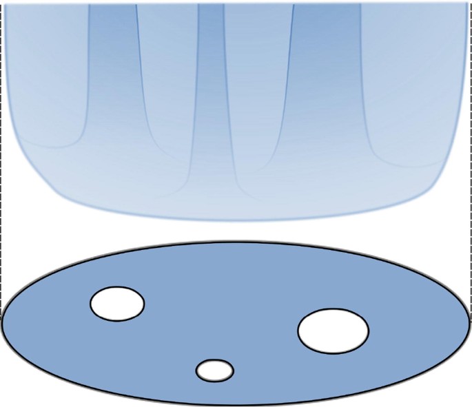

    

    Ω _t with many holes

    Finally, if a planar domain has countably many holes, we can arrange so that the holes disappear on a dense set of times. We get a smoothly evolving graph whose mean curvature is unbounded at all times.

7.2 Results

Let us consider mean curvature flow for graphs defined on a relatively open set

$$\displaystyle \begin{aligned} \varOmega\equiv\bigcup\limits_{t\ge0}\varOmega_t\times\{t\} \subset{\mathbb{R}}^{n+1}\times[0,\infty). \end{aligned} $$

(18)

Our existence result for bounded domains is

Theorem 12 (Existence)

Let $A\subset {\mathbb {R}}^{n+1}$ be a bounded open set and $u_0\colon A\to {\mathbb {R}}$ a locally Lipschitz continuous function with u ₀(x) →∞ for x → x ₀ ∈ ∂A.

Then there exists (Ω, u), where $\varOmega \subset {\mathbb {R}}^{n+1}\times [0,\infty )$ is relatively open, such that $u\colon \varOmega \to {\mathbb {R}}$ solves graphical mean curvature flow

$$\displaystyle \begin{aligned}\dot u=\sqrt{1+|Du|{}^2}\cdot \operatorname{\mathrm{div}}\left(\frac{Du} {\sqrt{1+|Du|{}^2}}\right)\quad \mathit{\text{in }}\varOmega\cap\{t>0\},\end{aligned}$$

u is smooth for t > 0 and continuous up to t = 0, Ω ₀ = A, u(⋅, 0) = u ₀ in A and u(x, t) →∞ as (x, t) → (x ₀, t ₀) ∈ ∂Ω, where ∂Ω is the relative boundary of Ω in ${\mathbb {R}}^{n+1}\times [0,\infty )$.

Such smooth solutions yield weak solutions to mean curvature flow. We have

Theorem 13 (Weak Flow)

Let (A, u ₀) and (Ω, u) be as in Theorem 12 . Let $\partial \mathscr D_t$ be the level set evolution of ∂Ω ₀ with $\mathscr D_0=\varOmega _0$ . If $\partial \mathscr D_t$ does not fatten, the measure theoretic boundaries of Ω _t and $\mathscr D_t$ coincide for every t ≥ 0.

Here, $\mathscr D_t=\left \{x\in {\mathbb {R}}^{n+1}\colon w(x,t)<0\right \}$ and w solves $\dot w=|Dw|\cdot \operatorname {\mathrm {div}}\left (\frac {Dw}{|Dw|}\right )$ as in Remark 5. The equation is solved in the viscosity sense, see e.g. [5, 12] for more details.

7.3 Strategy of Proof

Proof (Strategy of the Proof of Theorem 12)

• (i) Fix L > 0. Then there exists a solution with initial value $\min \{u_0,L\}$ for all t ∈ [0, ∞], see [11].

• (ii) If L ₁ < L, we prove a priori estimates for the part of the evolving graphs which is below L ₁. This is done in Theorem 16 for the (spatial) first order derivatives of u. See Theorem 17 for the second derivative bounds. Similar techniques imply bounds for all higher derivatives.

• (iii) We let L →∞ and use a variant of the Theorem of Arzelà-Ascoli to pass to a subsequence which converges to our solution.

□

Proof (Sketch of the Strategy of the Proof of Theorem 13)

In the following sketch of a proof we try to give an idea of the argument without mentioning technical details, e.g. approximations or fattening. None of the steps works exactly as described below.

• (i) The constructed solution $\operatorname {\mathrm {graph}} u(\cdot ,t)$ corresponds to a level-set solution.

• (ii) The level-set solution starting from $\partial A\times {\mathbb {R}}$ is an outer barrier to the graphical solution $\operatorname {\mathrm {graph}} u(\cdot ,t)$. Observe that Ω _t is the projection of the evolving graph at time t to ${\mathbb {R}}^{n+1}$. Hence Ω _t is contained in the level-set evolution of A.

• (iii) By shifting the level set solution downwards, we obtain convergence to the level set solution starting with the cylinder $\partial A\times {\mathbb {R}}$. This prevents $\operatorname {\mathrm {graph}} u(\cdot ,t)$ from detaching near infinity from the evolution of the cylinder.

□

7.4 The A Priori Estimates

Recall the definition $\mathrm {v}=\sqrt {1+|Du|{ }^2}$, where we consider u as a function defined on some subset of ${\mathbb {R}}^{n+1}\times [0,\infty )$.

Let η := (η _α) = (0, …, 0, 1). In the following, whenever quantities like v or |A|² are involved, we consider u and v as functions on the evolving hypersurfaces rather than as functions depending on $(x,t)\in {\mathbb {R}}^{n+1}\times [0,\infty )$, i.e. we consider u := X ^α η _α and v := −〈ν, η〉⁻¹.

Theorem 14

Let X be a solution to mean curvature flow. Then we have the following evolution equations

$$\displaystyle \begin{aligned} \left(\tfrac d{dt}-\varDelta\right) u=&\,0,\\ \left(\tfrac d{dt}-\varDelta\right) \mathrm{v}=&\,-|A|{}^2\mathrm{v}-\tfrac{2}{\mathrm{v}}|\nabla \mathrm{v}|{}^2,\\ \left(\tfrac d{dt}-\varDelta\right) |A|{}^2=&\,-2|\nabla A|{}^2+2|A|{}^4,\\ \left(\tfrac d{dt}-\varDelta\right) \mathscr{G}\le&\,-2k\cdot\mathscr{G}^2 -2{\varphi} \mathrm{v}^{-3}\langle\nabla \mathrm{v},\nabla \mathscr{G}\rangle, \end{aligned} $$

where $\mathscr {G} ={\varphi }|A|{ }^2 \equiv \frac {\mathrm {v}^2}{1-k\mathrm {v}^2}|A|{ }^2$ and k > 0 is chosen so that $k\mathrm {v}^2\le \frac {1}{2}$ in the domain considered.

Proof

For mean curvature flow, we have F ^ij = g ^ij. This implies F ^ij h _ij = H. In view of (13), we deduce $\left (\tfrac d{dt}-\varDelta \right ) X=0$ and $\left (\tfrac d{dt}-\varDelta \right ) u=0$.

For the evolution equation of w := |A|², we calculate

For the remaining claims see [10, 11]. □

Assumption 15

For the proof of the a priori estimates, we will assume that

$$\displaystyle \begin{aligned}u\colon{\mathbb{R}}^{n+1}\times[0,\infty)\to{\mathbb{R}}\end{aligned}$$

is a smooth solution to mean curvature flow such that for any T > 0 there exists R > 0 such that for all t ∈ [0, T]

$$\displaystyle \begin{aligned}\{x\colon u(x,t)\le 0\}\subset B_R(0).\end{aligned}$$

In order to be able to consider smooth solutions, a few extra constructions are necessary.

Theorem 16 (C ¹-Estimates)

Let u be as in Assumption 15 . Then

$$\displaystyle \begin{aligned}\mathrm{v}(-u)^2=\mathrm{v} u^2\le\max\limits_{\genfrac{}{}{0pt} {}{t=0}{\{u<0\}}}\mathrm{v} u^2\end{aligned}$$

at points where u < 0.

Here and in the following, it is often possible to increase the exponent of − u.

Proof

According to Theorem 14, w := vu ² fulfills

$$\displaystyle \begin{aligned} \dot w=&\,\dot{\mathrm{v}} u^2+2\mathrm{v} u\dot u,\\ w_i=&\,\mathrm{v}_iu^2+2\mathrm{v} uu_i,\\ w_{ij}=&\,\mathrm{v}_{ij}u^2+2\mathrm{v} uu_{ij} +2\mathrm{v} u_iu_j +2u(\mathrm{v} _iu_j+\mathrm{v} _ju_i),\\ \left(\tfrac d{dt}-\varDelta\right) w=&\,u^2\left(\tfrac d{dt}-\varDelta\right) \mathrm{v} -2\mathrm{v} |\nabla u|{}^2-4u\langle\nabla \mathrm{v},\nabla u\rangle\\ =&\,u^2\left(-\mathrm{v}|A|{}^2-\frac{2}{\mathrm{v}}|\nabla \mathrm{v} |{}^2\right) -2\mathrm{v} |\nabla u|{}^2 -4\left\langle\frac{u}{\sqrt{\mathrm{v}}}\nabla \mathrm{v},\sqrt{\mathrm{v}}\nabla u\right\rangle\\ \le&\,-u^2\mathrm{v}|A|{}^2\le0. \end{aligned} $$

The estimate follows from the maximum principle applied to w in the domain where u < 0. □

Remark 11

We recommend thinking of Theorem 16 as an estimate for v(−u)².

Corollary 4

Let u be as in Assumption 15 . Then

$$\displaystyle \begin{aligned}\mathrm{v}\le\max\limits_{\genfrac{}{}{0pt}{}{t=0}{\{u<0\}}}\mathrm{v} u^2\end{aligned}$$

at points where u ≤−1.

Exercise 17

Consider v(−u) to obtain similar C ¹-estimates.

Remark 12

Corollaries similar to Corollary 4 also hold for the following a priori estimates for points with u ≤−ε < 0 or t ≥ ε > 0. We do not write them down explicitly.

In Theorem 16 and later, the result still holds if we replace every u by u − h for any constant h.

Remark 13

For later use, we estimate derivatives of u and v,

$$\displaystyle \begin{aligned} |\nabla u|{}^2=&\,\eta_\alpha X^\alpha_ig^{ij}X^\beta_j\eta_\beta =\eta_\alpha\left(\delta^{\alpha\beta} -\nu^\alpha\nu^\beta\right)\eta_\beta =1-\mathrm{v}^{-2}\le 1 \end{aligned} $$

and, according to (3),

$$\displaystyle \begin{aligned} |\nabla \mathrm{v} |{}^2=&\,\left(\left(-\eta_\alpha\nu^\alpha\right)^{-1}\right)_i g^{ij}\left(\left(-\eta_\beta\nu^\beta\right)^{-1}\right)_j =\mathrm{v} ^4\eta_\alpha X^\alpha_kh^k_ig^{ij} h^l_jX^\beta_l\eta_\beta \\ \le&\,\mathrm{v}^4|A|{}^2 \le \mathrm{v}^2{\varphi}|A|{}^2 =\mathrm{v}^2\mathscr{G}. \end{aligned} $$

We therefore obtain

$$\displaystyle \begin{aligned} |\langle\nabla u,\nabla \mathrm{v}\rangle| \le&\,|\nabla u|\cdot|\nabla \mathrm{v}| \le \mathrm{v}^2|A|\le \mathrm{v}\sqrt{\mathscr{G}}. \end{aligned} $$

Theorem 17 (C ²-Estimates)

Let u be as in Assumption 15.

• (i) Then there exist λ > 0, c > 0 and k > 0 (the constant in φ and implicitly in $\mathscr {G}$ ), depending on the C ¹ -estimates, such that

  $$\displaystyle \begin{aligned}tu^4\mathscr{G}+\lambda u^2\mathrm{v}^2\le ct+\sup\limits_{\genfrac{}{}{0pt}{}{t=0}{\{u<0\}}} \lambda u^2\mathrm{v}^2\end{aligned}$$

  at points where u < 0 and 0 < t ≤ 1.

• (ii) Moreover, if u is in C ² initially, we get C ² -estimates up to t = 0: Then there exists c > 0, depending only on the C ¹ -estimates, such that

  $$\displaystyle \begin{aligned}u^4\mathscr{G}\le ct+\sup\limits_{\genfrac{}{}{0pt}{}{t=0}{\{u<0\}}}u^4\mathscr{G}\end{aligned}$$

  at points where u < 0.

Proof

In order to prove both parts simultaneously, we set

$$\displaystyle \begin{aligned}w:=(\mu t+(1-\mu))u^4\mathscr{G}+\lambda u^2\mathrm{v}^2 \equiv\mu_tu^4\mathscr{G}+\lambda u^2\mathrm{v}^2.\end{aligned}$$

If we set μ = 1, we obtain μ _t = t and later the first claim, if μ = λ = 0, we get μ _t = 1 and deduce in the following the second claim. We calculate

$$\displaystyle \begin{aligned} \dot w=&\,\mu u^4\mathscr{G} +4\mu_tu^3\mathscr{G}\dot u+\mu_tu^4\dot{\mathscr{G}} +2\lambda \mathrm{v}^2u\dot u +2\lambda u^2\mathrm{v}\dot{\mathrm{v}},\\ w_i=&\,4\mu_tu^3\mathscr{G} u_i +\mu_tu^4\mathscr{G}_i +2\lambda \mathrm{v}^2uu_i +2\lambda u^2\mathrm{v} \mathrm{v}_i,\\ w_{ij}=&\,4\mu_tu^3\mathscr{G} u_{ij} +\mu_tu^4\mathscr{G}_{ij} +2\lambda \mathrm{v} ^2uu_{ij} +2\lambda u^2\mathrm{v}\mathrm{v}_{ij} +12\mu_tu^2\mathscr{G} u_iu_j\\ &\,+4\mu_tu^3(\mathscr{G}_iu_j+\mathscr{G}_ju_i) +2\lambda \mathrm{v}^2u_iu_j +2\lambda u^2 \mathrm{v} _i\mathrm{v}_j\\ &\, +4\lambda u \mathrm{v} (u_i\mathrm{v}_j+u_j\mathrm{v}_i),\\ \mu_tu^3\nabla\mathscr{G}=&\,\frac{1}{u}\nabla w -4\mu_tu^2\mathscr{G}\nabla u -2\lambda \mathrm{v} ^2\nabla u -2\lambda u\mathrm{v}\nabla \mathrm{v},\\ \left(\tfrac d{dt}-\varDelta\right) w\le&\,\mu{u^4\mathscr{G}} +\mu_tu^4\left(-2k\cdot\mathscr{G}^2-2{\varphi} \mathrm{v}^{-3}\langle\nabla \mathrm{v} ,\nabla\mathscr{G}\rangle\right)\\ &\, +2\lambda u^2\mathrm{v}\left(-|A|{}^2\mathrm{v} -\tfrac{2}{\mathrm{v}}|\nabla \mathrm{v}|{}^2\right) -12\mu_tu^2\mathscr{G}|\nabla u|{}^2\\ &\,-8\mu_tu^3\langle\nabla\mathscr{G},\nabla u\rangle -2\lambda \mathrm{v}^2|\nabla u|{}^2 -2\lambda u^2|\nabla \mathrm{v}|{}^2 -8\lambda u\mathrm{v}\langle\nabla u,\nabla \mathrm{v}\rangle. \end{aligned} $$

In the following, we will use the notation 〈∇w, b〉 with a generic vector b. The constants c are allowed to depend on $\sup \{|u|\colon u<0\}$ (which does not exceed its initial value) and the C ¹-estimates. It may also depend on an upper bound for t, but we assume that 0 < t ≤ 1 whenever t appears explicitly. I.e., we suppress dependence on already estimated quantities.

We estimate the terms involving $\nabla \mathscr {G}$ separately. Let ε > 0 be a constant. We fix its value below. Using Remark 13 for estimating terms, we get

$$\displaystyle \begin{aligned} -2{\varphi}\mu_tu^4\mathrm{v} ^{-3}&\langle\nabla \mathrm{v} ,\nabla\mathscr{G}\rangle\\ =&\,-2\frac{{\varphi} u}{\mathrm{v}^3}\left\langle\nabla \mathrm{v},\frac{1}{u}\nabla w-4\mu_tu^2\mathscr{G}\nabla u-2\lambda \mathrm{v}^2\nabla u-2\lambda u\mathrm{v}\nabla \mathrm{v}\right\rangle\\ \le&\,\langle\nabla w,b\rangle +8\mu_t\frac{{\varphi} |u|{}^3}{\mathrm{v}}\mathscr{G}|A| +4\lambda{\varphi} \mathrm{v}|u||A| +4\frac{\lambda{\varphi} u^2}{\mathrm{v}^2} |\nabla \mathrm{v}|{}^2\\ =&\,\langle\nabla w,b\rangle +8\mu_t{\varphi}^2\frac{|u|{}^3\mathscr{G}^{3/2}}{{\varphi}^{3/2}} \frac{1}{\mathrm{v}} +4\lambda{\varphi}\mathrm{v}|u||A| +\lambda u^2|\nabla\mathrm{v}|{}^2\cdot4\frac{\varphi}{\mathrm{v}^2}\\ \le&\,\langle\nabla w,b\rangle +{\varepsilon}\mu_tu^4\mathscr{G}^2 +{\varepsilon}\lambda u^2\mathrm{v}^2|A|{}^2 +\lambda u^2|\nabla \mathrm{v}|{}^2\cdot 4\frac{{\varphi}}{\mathrm{v}^2}\\ &\,+c({\varepsilon},\lambda),\\ -8\mu_tu^3&\langle\nabla\mathscr{G},\nabla u\rangle\\ =&\,-8\left\langle\nabla u,\frac{1}{u}\nabla w -4\mu_tu^2\mathscr{G}\nabla u -2\lambda \mathrm{v}^2\nabla u -2\lambda u\mathrm{v}\nabla \mathrm{v}\right\rangle\\ \le&\,\langle\nabla w,b\rangle +32\mu_tu^2\mathscr{G}+16\lambda \mathrm{v}^2+16\lambda |u|\mathrm{v}^3|A|\\ \le&\,\langle\nabla w,b\rangle +{\varepsilon}\mu_tu^4\mathscr{G}^2 +{\varepsilon}\lambda u^2\mathrm{v}^2|A|{}^2 +c({\varepsilon},\lambda). \end{aligned} $$

We obtain

$$\displaystyle \begin{aligned} \left(\tfrac d{dt}-\varDelta\right) w\le&\,\mu{u^4\mathscr{G}} +\mu_tu^4\mathscr{G}^2(-2k+2{\varepsilon}) +\langle\nabla w,b\rangle\\ &\,+\lambda u^2\mathrm{v}^2|A|{}^2(-2+3{\varepsilon}) +\lambda u^2|\nabla \mathrm{v}|{}^2\left(4\frac{\varphi}{\mathrm{v}^2}-6\right) +c({\varepsilon},\lambda). \end{aligned} $$

Let us assume that k > 0 is chosen so small that $k\mathrm {v}^2\le \frac {1}{3}$ in {u < 0}. This implies φ ≤ 2v². We may assume that λ ≥ 2u ² in {u < 0} and get $\mu {u^4\mathscr {G}}\le \frac {1}{2}\lambda u^2{\varphi }|A|{ }^2 \le \lambda u^2\mathrm {v}^2|A|{ }^2$. We get

$$\displaystyle \begin{aligned}4\frac{\varphi}{\mathrm{v}^2}-6 =\frac{4}{1-k\mathrm{v}^2} -6\le 0.\end{aligned}$$

Finally, fixing ε > 0 sufficiently small, we obtain

$$\displaystyle \begin{aligned}\left(\tfrac d{dt}-\varDelta\right) w\le\langle\nabla w,b\rangle +c.\end{aligned}$$

Now, both claims follow from the maximum principle. □

Appendices

Appendix 1: Parabolic Maximum Principles

The following maximum principle is fairly standard. For non-compact, strict or other maximum principles, we refer to [11] or [24], respectively.

We will use C ^2;1 for the space of functions that are two times continuously differentiable with respect to the space variables and once continuously differentiable with respect to the time variable.

Theorem 18 (Weak Parabolic Maximum Principle)

Let $\varOmega \subset {\mathbb {R}}^n$ be open and bounded and T > 0. Let a ^ij , b ⁱ ∈ L ^∞(Ω × [0, T]). Let a ^ij be strictly elliptic, i.e. a ^ij(x, t) > 0 in the sense of matrices. Let $u\in C^{2;1}(\varOmega \times [0,T))\times C^0\left (\overline \varOmega \times [0,T]\right )$ fulfill

$$\displaystyle \begin{aligned}\dot u\le a^{ij}u_{ij}+b^iu_i\quad \mathit{\text{in }}\varOmega\times(0,T).\end{aligned}$$

Then we get for (x, t) ∈ Ω × (0, T)

$$\displaystyle \begin{aligned}u(x,t)\le\sup\limits_{\mathscr P\left(\varOmega\times(0,T)\right)} u,\end{aligned}$$

where $\mathscr P\left (\varOmega \times (0,T)\right ):=(\varOmega \times \{0\}) \cup (\partial \varOmega \times (0,T))$.

Proof

• (i) Let us assume first that $\dot u<a^{ij}u_{ij}+b^iu_i$ in Ω × (0, T). If there exists a point (x ₀, t ₀) ∈ Ω × (0, T) such that $u(x_0,t_0)>\sup \limits _{\mathscr P\left (\varOmega \times (0,T)\right )} u$, we find (x ₁, t ₁) ∈ Ω × (0, T) and t ₁ minimal such that u(x ₁, t ₁) = u(x ₀, t ₀). At (x ₁, t ₁), we have $\dot u\ge 0$, u _i = 0 for all 1 ≤ i ≤ n, and u _ij ≤ 0 (in the sense of matrices). This, however, is impossible in view of the evolution equation.

• (ii) Define for 0 < ε the function v := u − εt. It fulfills the differential inequality

  $$\displaystyle \begin{aligned}\dot{\mathrm{v}} =\dot u-{\varepsilon}<\dot u\le a^{ij}u_{ij}+b^iu_i =a^{ij}\mathrm{v}_{ij}+b^i\mathrm{v}_i.\end{aligned}$$

  Hence, by the previous considerations,

  $$\displaystyle \begin{aligned}u(x,t)-{\varepsilon} t=\mathrm{v}(x,t)\le\sup\limits_{\mathscr P(\varOmega\times(0,T))} \mathrm{v} =\sup\limits_{\mathscr P(\varOmega\times(0,T))} u-{\varepsilon} t\end{aligned}$$

  and the result follows as .

□

There is also a parabolic maximum principle for tensors, see [19, Theorem 9.1]. (See the AMS-Review for a small correction of the proof.)

A tensor N _ij depending smoothly on M _ij and g _ij, involving contractions with the metric, is said to fulfill the null-eigenvector condition, if N _ijvⁱv^j ≥ 0 for all null-eigenvectors v of M _ij.

Theorem 19

Let (M _ij)_i,j be a tensor, defined on a closed Riemannian manifold (M, g(t)), fulfilling

$$\displaystyle \begin{aligned}{\frac{\partial}{\partial t}} M_{ij}=\varDelta M_{ij}+b^k\nabla_kM_{ij}+N_{ij}\end{aligned}$$

on a time interval [0, T), where b is a smooth vector field and N _ij fulfills the null-eigenvector condition. If M _ij ≥ 0 at t = 0, then M _ij ≥ 0 for 0 ≤ t < T.

Appendix 2: Some Linear Algebra

Lemma 14

We have

$$\displaystyle \begin{aligned}\frac\partial{\partial a_{ij}}\det(a_{rs}) =\det(a_{rs})a^{ji},\end{aligned}$$

if a _ij is invertible with inverse a ^ij , i.e. if $a^{ij}a_{jk}=\delta ^i_k$.

Proof

It suffices to prove that the claimed equality holds when we multiply it with a _ik and sum over i. Hence, we have to show that

$$\displaystyle \begin{aligned}\frac\partial{\partial a_{ij}} \det(a_{rs})a_{ik}=\det(a_{rs})\delta^j_k.\end{aligned}$$

We get

$$\displaystyle \begin{aligned}\frac\partial{\partial a_{ij}}\det(a_{rs})= \det\begin{pmatrix} a_{1\,1} & \hdots & a_{1\,j-1} & 0 & a_{1\,j+1} & \hdots & a_{1\,n}\\ \vdots & & \vdots & \vdots & \vdots & & \vdots\\ a_{i-1\,1} & \hdots & a_{i-1\,j-1} & 0 & a_{i-1\,j+1} & \hdots & a_{i-1\,n}\\ 0 & \hdots & 0 & 1 & 0 & \hdots & 0\\ a_{i+1\,1} & \hdots & a_{i+1\,j-1} & 0 & a_{i+1\,j+1} & \hdots & a_{i+1\,n}\\ \vdots & & \vdots & \vdots & \vdots & & \vdots\\ a_{n\,1} & \hdots & a_{n\,j-1} & 0 & a_{n\,j+1} & \hdots & a_{n\,n}\\ \end{pmatrix}.\end{aligned}$$

and thus

$$\displaystyle \begin{aligned} \frac\partial{\partial a_{ij}}\det(a_{rs})\cdot a_{ik}=& \det\begin{pmatrix} 0&\hdots&0&a_{1\,k}&0&\hdots&0\\ a_{2\,1}&\hdots&a_{2\,j-1}&0&a_{2\,j+1}&\hdots&a_{2\,n}\\ \vdots&&\vdots&\vdots&\vdots&&\vdots\\ a_{n\,1}&\hdots&a_{n\,j-1}&0&a_{n\,j+1}&\hdots&a_{n\,n} \end{pmatrix}\\ &+\det\begin{pmatrix} a_{1\,1}&\hdots&a_{1\,j-1}&0&a_{1\,j+1}&\hdots&a_{1\,n}\\ 0&\hdots&0&a_{2\,k}&0&\hdots&0\\ a_{3\,1}&\hdots&a_{3\,j-1}&0&a_{3\,j+1}&\hdots&a_{3\,n}\\ \vdots&&\vdots&\vdots&\vdots&&\vdots\\ a_{n\,1}&\hdots&a_{n\,j-1}&0&a_{n\,j+1}&\hdots&a_{n\,n} \end{pmatrix}\\ &+\hdots\\ =&\det\begin{pmatrix} a_{1\,1}&\hdots&a_{1\,j-1}&a_{1\,k}&a_{1\,j+1}&\hdots&a_{1\,n}\\ a_{2\,1}&\hdots&a_{2\,j-1}&0&a_{2\,j+1}&\hdots&a_{2\,n}\\ \vdots&&\vdots&\vdots&\vdots&&\vdots\\ a_{n\,1}&\hdots&a_{n\,j-1}&0&a_{n\,j+1}&\hdots&a_{n\,n} \end{pmatrix}\\ &+\det\begin{pmatrix} a_{1\,1}&\hdots&a_{1\,j-1}&0&a_{1\,j+1}&\hdots&a_{1\,n}\\ a_{2\,1}&\hdots&a_{2\,j-1}&a_{2\,k}&a_{2\,j+1}&\hdots&a_{2\,n}\\ a_{3\,1}&\hdots&a_{3\,j-1}&0&a_{3\,j+1}&\hdots&a_{3\,n}\\ \vdots&&\vdots&\vdots&\vdots&&\vdots\\ a_{n\,1}&\hdots&a_{n\,j-1}&0&a_{n\,j+1}&\hdots&a_{n\,n} \end{pmatrix}\\ &+\hdots\\ =&\det\begin{pmatrix} a_{1\,1}&\hdots&a_{1\,j-1}&a_{1\,k}&a_{1\,j+1}&\hdots&a_{1\,n}\\ \vdots&&\vdots&\vdots&\vdots&&\vdots\\ a_{n\,1}&\hdots&a_{n\,j-1}&a_{n\,k}&a_{n\,j+1}&\hdots&a_{n\,n} \end{pmatrix}\\ =&\delta^j_k\det(a_{rs}). \end{aligned} $$

□

Lemma 15

Let a _ij(t) be differentiable in t with inverse a ^ij(t). Then

$$\displaystyle \begin{aligned}{\frac{d}{dt}} a^{ij}=-a^{ik}a^{lj}{\frac{d}{dt}} a_{kl}.\end{aligned}$$

Proof

We have

$$\displaystyle \begin{aligned}a^{ik}a_{kj}=\delta^i_j.\end{aligned}$$

There exists $\tilde a^{ij}$ such that

$$\displaystyle \begin{aligned}a_{ik}\tilde a^{kj}=\delta^j_i.\end{aligned}$$

Then $a^{ij}=\tilde a^{ij}$, as

$$\displaystyle \begin{aligned}a^{ij}=a^{ik}\delta^j_k=a^{ik}\left(a_{kl}\tilde a^{lj}\right) =\left(a^{ik}a_{kl}\right)\tilde a^{lj}=\tilde a^{ij}.\end{aligned}$$

We differentiate and obtain

$$\displaystyle \begin{aligned}0={\frac{d}{dt}}\delta^i_j={\frac{d}{dt}}\left(a^{ik}a_{kj}\right) ={\frac{d}{dt}} a^{ik}a_{kj}+a^{ik}{\frac{d}{dt}} a_{kj}.\end{aligned}$$

Hence

$$\displaystyle \begin{aligned}{\frac{d}{dt}} a^{il}={\frac{d}{dt}} a^{ik}\delta^l_k ={\frac{d}{dt}} a^{ik}a_{kj}a^{jl} =-a^{ik}{\frac{d}{dt}} a_{kj}a^{jl}.\end{aligned}$$

□

References

B. Andrews, Contraction of convex hypersurfaces in Euclidean space. Calc. Var. Partial Differ. Equ. 2(2), 151–171 (1994)
B. Andrews, Gauss curvature flow: the fate of the rolling stones. Invent. Math. 138(1), 151–161 (1999)
B. Andrews, P. Guan, L. Ni, Flow by powers of the Gauss curvature. Adv. Math. 299, 174–201 (2016)
S. Brendle, K. Choi, P. Daskalopoulos, Asymptotic behavior of flows by powers of the Gaussian curvature. Acta Math. 219, 1–16 (2017)
Y.G. Chen, Y. Giga, S. Goto, Uniqueness and existence of viscosity solutions of generalized mean curvature flow equations. J. Differ. Geom. 33(3), 749–786 (1991)
B. Chow, Deforming convex hypersurfaces by the nth root of the Gaussian curvature. J. Differ. Geom. 22(1), 117–138 (1985)
J. Clutterbuck, Parabolic equations with continuous initial data (2004). arXiv:math.AP/0504455
J. Clutterbuck, O.C. Schnürer, F. Schulze, Stability of translating solutions to mean curvature flow. Calc. Var. Partial Differ. Equ. 29(3), 281–293 (2007)
T.H. Colding, W.P. Minicozzi II, Sharp estimates for mean curvature flow of graphs. J. Reine Angew. Math. 574, 187–195 (2004)
K. Ecker, Regularity Theory for Mean Curvature Flow. Progress in Nonlinear Differential Equations and Their Applications, vol. 57 (Birkhäuser Boston Inc., Boston, 2004)
K. Ecker, G. Huisken, Interior estimates for hypersurfaces moving by mean curvature. Invent. Math. 105(3), 547–569 (1991)
L.C. Evans, J. Spruck, Motion of level sets by mean curvature. I. J. Differ. Geom. 33(3), 635–681 (1991)
M.E. Feighn, Separation properties of codimension-1 immersions. Topology 27(3), 319–321 (1988)
W.J. Firey, Shapes of worn stones. Mathematika 21, 1–11 (1974)
M. Gage, R.S. Hamilton, The heat equation shrinking convex plane curves. J. Differ. Geom. 23(1), 69–96 (1986)
C. Gerhardt, Flow of nonconvex hypersurfaces into spheres. J. Differ. Geom. 32(1), 299–314 (1990)
C. Gerhardt, Curvature Problems. Series in Geometry and Topology, vol. 39 (International Press, Somerville, 2006)
M.A. Grayson, The heat equation shrinks embedded plane curves to round points. J. Differ. Geom. 26(2), 285–314 (1987)
R.S. Hamilton, Three-manifolds with positive Ricci curvature. J. Differ. Geom. 17(2), 255–306 (1982)
G. Huisken, Flow by mean curvature of convex surfaces into spheres. J. Differ. Geom. 20(1), 237–266 (1984)
G. Huisken, T. Ilmanen, The inverse mean curvature flow and the Riemannian Penrose inequality. J. Differ. Geom. 59(3), 353–437 (2001)
G. Huisken, A. Polden, Geometric evolution equations for hypersurfaces, in Calculus of Variations and Geometric Evolution Problems (Cetraro, 1996). Lecture Notes in Mathematics, vol. 1713 (Springer, Berlin, 1999), pp. 45–84
J.A. McCoy, The surface area preserving mean curvature flow. Asian J. Math. 7(1), 7–30 (2003)
M.H. Protter, H.F. Weinberger, Maximum Principles in Differential Equations (Springer, New York, 1984). Corrected reprint of the 1967 original
M. Sáez Trumper, O.C. Schnürer, Mean curvature flow without singularities. J. Differ. Geom. 97(3), 545–570 (2014)
O.C. Schnürer, The Dirichlet problem for Weingarten hypersurfaces in Lorentz manifolds. Math. Z. 242(1), 159–181 (2002)
O.C. Schnürer, Surfaces contracting with speed |A|2. J. Differ. Geom. 71(3), 347–363 (2005)
O.C. Schnürer, Surfaces expanding by the inverse Gauß curvature flow. J. Reine Angew. Math. 600, 117–134 (2006)
N. Stavrou, Selfsimilar solutions to the mean curvature flow. J. Reine Angew. Math. 499, 189–198 (1998)
C. Sturm, Mémoire sur la résolution des équations numeriques. Bull. Sci. Math. Ferussac 11, 419–422 (1829)
K. Tso, Deforming a hypersurface by its Gauss-Kronecker curvature. Commun. Pure Appl. Math. 38(6), 867–882 (1985)
J.I.E. Urbas, An expansion of convex hypersurfaces. J. Differ. Geom. 33(1), 91–125 (1991)
Author information
Authors and Affiliations
Corresponding author
Editor information
Editors and Affiliations