
Abstract
Publicly available bioassay data often contains errors. Curating massive bioassay data, especially high-throughput screening (HTS) data, for Quantitative Structure-Activity Relationship (QSAR) modeling requires the assistance of automated data curation tools. Using automated data curation tools are beneficial to users, especially ones without prior computer skills, because many platforms have been developed and optimized based on standardized requirements. As a result, the users do not need to extensively configure the curation tool prior to the application procedure. In this chapter, a freely available automatic tool to curate and prepare HTS data for QSAR modeling purposes will be described.
Access provided by CONRICYT – Journals CONACYT. Download protocol PDF
Key words
1 Introduction
A typical high-throughput screening (HTS) data set can contain over 10,000 compounds (e.g., Antioxidant Response Element assay data listed as PubChem AID 743219). Although they are potential resources for developing Quantitative Structure-Activity Relationship (QSAR) models, normally these public HTS data sets cannot be used directly for modeling purposes due to the presence of duplicates, artifacts, and other issues. There are public chemical data repositories such as PubChem , ChemSpider, and ChEMBL that contain lots of HTS data available for download, but the original data stored in these resources still need further curation. However, HTS data sets are so large that it is very inefficient, and usually ineffective, to process all the data points manually. The assistance of automated tools is highly recommended.
Chemical structure curation and standardization is an integral step in QSAR modeling. This step is essential since it is likely the same compounds will be represented differently among different sources. For example, organic compounds could be drawn with implicit or explicit hydrogens, in aromatized or Kekulé form, as well as in different tautomeric forms. These differences in chemical structure representations could influence the computed chemical descriptor values for the same compound and greatly affect the usefulness and quality of the resulting QSAR models. Furthermore, the existence of inorganic compounds and mixtures, which are not suitable for traditional QSAR modeling studies, also limits the use of public HTS data.
Another issue with HTS data is that it is very common for it to have an unbalanced distribution of activities, where there are substantially more inactive than active compounds. This unbalanced distribution of activities (i.e., low active ratio) could result in biased QSAR model predictions. Data sampling, an approach that selects and analyzes a subset of the overall data, can resolve this issue. The specific data sampling method that will be discussed in this chapter is down-sampling , since it is most relevant to HTS data processing. Down-sampling is an approach that ignores most of the data points that are in the largest activity category. This will allow you to select a sample of the inactive compounds from the data set to balance the distribution of activities for modeling. Furthermore, smaller data sets are easier to manage and, in most cases, more informative since it captures the most important elements of the data.
In this chapter, an automatic data curation process that can standardize/harmonize chemical structures and down-sample the results of a large HTS data set will be described. The approaches to construct the modeling and validations sets, including balancing the HTS activity via down-sampling, were configured using Konstanz Information Min er (KNIME ver. 2.10.1) (www.knime.org) workflows that utilize the two most common approaches for selecting a sample size: random and rational selection methods. These processes utilize basic statistical approaches [1] and will transform an original public HTS data set into a curated format suitable for QSAR model development and other relevant in silico modeling efforts. The quantitative high-throughput screening (qHTS) Antioxidant Response Element assay data obtained from PubChem (PubChem AID 743219) will be used to illustrate this data curation process.
2 Materials
Automated procedures to curate chemical structures and down-sample the large data set (i.e., HTS data) will be described in this chapter. All of the workflows were developed and executed in the open-source platform KNIME. The output files of the workflows are curated data sets with standardized structures that are ready to be processed by QSAR modeling tools. The workflows can be downloaded as a zip file at https://github.com/zhu-lab.
3 Methods
3.1 Prepare an Input File for the Curation Workflow
An input file should be a tab delimited multiple column txt file (FileName.txt) with a header to each column, where one column must contain the structure information as a SMILES code [3]. The input file (a sample file was provided within the zip file) should have at least three columns: ID, SMILES, and activity. If needed, other useful features of compounds (e.g., compound names) could also be included as extra columns.
3.2 Prepare the Curation Workflow
Install the KNIME software. It can be downloaded from www.knime.org. Download the curation workflow (https://github.com/zhu-lab/curation-workflow) and extract the zip file into a computer directory.
3.3 Configure the Workflow
In the File menu bar of KNIME, select “Import KNIME workflow…” to import the structure standardizer workflow into KNIME. Now in the pop-up window (Fig. 1), click on “Source: Select root directory,” find the computer directory that the zip file was extracted to. Select the destination directory, which will be where the output files will be saved to. In “Workflows:” select the “Structure Standardizer” workflow and click “Finish” (Fig. 2).

The KNIME “ Workflow Import Selection” window

A window of the KNIME “Structure Standardizer” workflow
3.4 Set Up Parameters and Run the Workflow
To open the workflow, double click on the Structure Standardizer in the “KNIME Explorer” window under “LOCAL (Local Workspace)” located in the top left side bar. At this time, the workflow will show up in the main space, which is called the workflow editor (see Note 1 ) Right click the “File Reader” node and select “Configure.” In the pop-up windows, input the valid file location of the input file that has been prepared in the previous step. Make sure the headers of the input file are read correctly. Click “OK” to save the changes and close the configuration window. Next, right click the “Java Edit Variable” node in the bottom left and change the variable v_dir to the directory of the folder where all the files are extracted in the second step. Then, configure sub-workflows individually by double clicking on each node. Within each sub-workflow, configure the Java Edit Variable node the same as described above. After closing the sub-workflow windows, the yellow lights on all the nodes should be on, indicating that the workflow is ready to be used. Click on the green “double-arrow button” located in the top menu bar to execute the whole workflow and the green lights on all nodes should be on. Three output files should have been generated in the same folder as the input file (FileName_fail.txt, FileName_std.txt, and FileName_warn.txt) (see Note 2 ). (Or the files will be in a folder directory substituting all spaces with % 20 if spaces are in the directory (e.g., if input file is in F:\Structure Standardizer\output, then output file would be in F:\Structure%20Standardizer\output).) The standardized compounds will be in canonical SMILES format (see Note 3 ). The file FileName_std.txt is the data set curated for modeling purposes.
3.5 Preparing the Chemical Descriptor File
With the chemical structures curated, the chemical descriptors can be calculated by using various descriptor generators, such as RDKit (http://www.rdkit.org/), Molecular Operating Environment® (MOE) (https://www.chemcomp.com/MOE-Molecular_Operating_Environment.htm), and Dragon® (http://www.talete.mi.it/products/dragon_description.htm) (see Note 4 ).
3.6 Preparing the Modeling and Validation Set Files
To develop a predictive QSAR model, the compound classifications in the modeling set need to be balanced (see Note 5 ) To this end, the inactive compounds of HTS data need to be down-sampled to be similar to the number of actives in the modeling set. There are two methods that can be applied for this purpose: random and rational selection.
The random selection approach will randomly select an equal number of inactive compounds compared to the actives. Figure 3a shows a KNIME workflow that could be used to randomly select compounds and partition the data set into modeling and validation sets (see Note 6 ). This workflow ensures that the relationships between each compound selected for the model development and validation purposes were not explicitly selected. To run the workflow, first input the curated file (e.g., the file FileName_std.txt) from previous step with a minimum of two columns for the ID and activity in the “File Reader” node. Then, right click on the activity column header to open the “Column Properties” and set the “Type” as “String.” The workflow has already been configured to randomly select 500 active and 500 inactive compounds; however, the numbers of active/inactive compounds can be changed. Click on the green “double-arrow button” located in the top menu bar to execute the whole workflow. Two files will be generated in the destination directory: ax_input_modeling.txt and ax_input_intValidating.txt. The ax_input_modeling.txt file contains the 500 active and 500 inactive compounds randomly selected to balance the distribution of activities in the modeling set. The ax_input_intValidating.txt file contains the remaining compounds (e.g., 458 active and 4026 inactive compounds from the sample data set) that could be used for validation purposes.

Example of KNINE workflow for selecting compounds and partitioning data set into modeling and validation sets using (a) random and (b) rational selection approaches
Compared to random selection, rational selection is also frequently used in down-sampling (see Note 7 ). Figure 3b shows a KNIME w orkflow that could be used to rationally select compounds for QSAR model development, based on the threshold defined using principal component analysis (see Note 8 ), and partition the data set into modeling and validation sets. The rational selection approach uses a quantitatively defined threshold of similarity to select inactive to active compounds. In this case, inactive compounds that share the same descriptor space of active compounds will be selected and successively define the applicability domain in the resulting QSAR models [2]. The KNIME workflow described here differs slightly from the random selection workflow described above in that it allows one to quantitatively define the similarity threshold using PCA. To run the workflow, first input the curated file (e.g., FileName_std.txt) from the previous step with columns for the ID, activity, and descriptors into the “File Reader” node. Then right click on the activity column header to open the “Column Properties” and set the “Type” to “String.” The workflow has already been configured to select 500 active and 500 inactive compounds and the numbers of active/inactive compounds can be changed. Click on the green “double-arrow button” located in the top menu bar to execute the whole workflow. Three files will be generated in the destination directory: ax_input_ratl_modeling.txt, ax_input_ratl_intValidating.txt, and ax_input_ratl_outAD.txt.
3.7 Verification: Visualizing the Chemical Space Covered by the Data Set Using Principal Components
After the modeling and validation sets are created, the chemical space (see Note 9 ) can be visualized. The chemical space of a data set can be shown in a 3-D plot using the first three principal components (of the descriptor space) generated from MOE chemical descriptors (see Note 10 ). In Fig. 4a, the chemical space using the first three principal components of the entire ARE d ata set 7034 compounds was plotted. Then, 500 active and 500 inactive compounds organized the chemical space for the modeling set, as shown in Fig. 4b. The inactive compounds were selected based on the chemical similarity to the actives, so the chemical space occupied by the modeling set is clearly different from the whole data set. Therefore, the predictions of resulting QSAR models should be considered reliable within the chemical space (i.e., the applicability domain ) of modeling set.

3-D plots of ARE data set using (a) all 7034 data points, and (b) modeling set using principal components 1–3 generated using 10 MOE descriptors
A principal component analysis was performed in KNIME o n all the active and inactive compounds in the ARE data set of 5484 compounds (Fig. 5). From the scatter plot of principal components 1 versus 2, it was noticeable that most of the compounds clustered at principal component 1 values between −0.2 and 0.3. Therefore, the applicability domain of the resulting model can be defined as any compound that falls within this range. To adjust this applicability domain in the KNIME workflow, adjust both “Row Splitter” nodes by right clicking the node, under “use range checking,” adjust the “lower bound” and “upper bound.” Under this condition 500 active and 500 inactive compounds within the range of −0.2 and 0.3 will be selected for the modeling set, while the others will be placed into the validation set. Compounds that were out of domain will be placed into the ax_input_ratl_outAD.txt file.

Example of KNIME workflow for visualizing the chemical space of all active and inactive compounds
4 Notes
-
1.
If you cannot find these windows, go to the “View” in the menu bar and select “Reset Perspective…”
-
2.
Description of the three output files:
FileName_fail.txt contains compounds that could neither be standardized nor be used in the QSAR modeling (e.g., mixtures, inorganics, and large molecules like polypeptides).
FileName_std.txt contains the remaining structurally standardized compounds in which the SMILES are curated as the canonical format.
FileName_warn.txt contains compounds with potential problems that require further review. For example, compounds with positive/negative charges need to be compared to their original structures to decide the correct structure information. These compounds with warnings will not be removed from the data set and are included in the FileName_std.txt file.
-
3.
Compounds in this file are curated, standardized, and represented in canonical form by removing metals, de-isomerizing tautomer, neutralizing salts and charges, de-aromatizing rings, and fulfill the requirements of QSAR modeling. For more information please look into the commented .smk files.
-
4.
The descriptor values of the whole data set need to be normalized between 0 and 1 before QSAR model development. Furthermore, if there are too many descriptors (e.g., the number of resulting Dragon descriptors is normally over 1000), it is necessary to reduce the number of descriptors to save computational time for model development. Performing a pairwise comparison between any two descriptor values is one way to find correlated and redundant descriptors. This can be done by constructing a scatter plot for every pair of descriptors and determining the Pearson’s product-moment coefficient for every pair [1].
-
5.
After the descriptor file is generated and optimized, it is needed to balance active/inactive classification ratio in the modeling set and prepare the activity file for modeling purpose. Normally the number of inactives is much larger than the number of actives in HTS data sets. For example, the ARE data set contains 958 active and 4,526 inactive compounds (Fig. 6).
Fig. 6 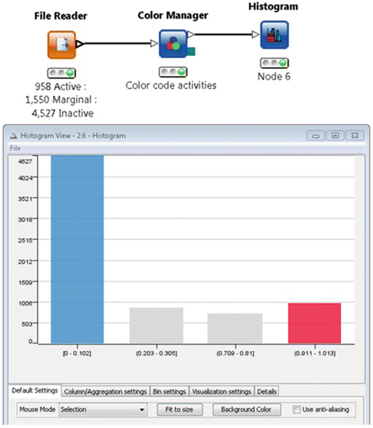
Example of KNIME histogram plot workflow and the resulting histogram plot showing the frequency of activity values 0 (inactive, blue), 0.25 to 0.50 (marginal, gray), and 1 (active, red)
-
6.
KNIME also has an “Equal Size Sampling” node that automatically down-samples the data set and it can be substituted into the workflow. However, it does not partition the data set into modeling and validation sets.
-
7.
It has been reported that there is little difference in the QSAR model performance resulting from these two methods (Martin et al. 2012). This method ensures that the test set will have structurally similar analogs in the modeling set, but this cannot be guaranteed for external set compounds. However, rational selection approach may be advantageous when the applicability domain of the QSAR model needs to be clearly defined (Golbraikh et al. 2003).
More information on random and rational selection and applicability domain can be found at: Martin TM, Harten P, Young DM, Muratov EN, Golbraikh A, Zhu H, et al. 2012. Does rational selection of training and test sets improve the outcome of QSAR modeling? J. Chem. Inf. Model. 52:2570–8; doi:10.1021/ci300338w.
Golbraikh A, Shen M, Xiao Z, Xiao Y-D, Lee K-H, Tropsha A. 2003. Rational selection of training and test sets for the development of validated QSAR models. J. Comput. Aided. Mol. Des. 17:241–53; doi:10.1023/A:1025386326946.
-
8.
Principal component analysis is a statistical method that reduces the dimensions of descriptors in a data set by finding groups of descriptor combinations. It also provides one of the most informative statistics about the data. The first principal component covers the largest amount of variance in the data set. Each consecutive principal component will cover another portion of the variance, but less than the previous one. Therefore, the combination of all principal components represents the total variance in the data set. And the total number of principal components is less than the number of descriptors. All these calculations can be done in software such as KNIME and MOE.
Typically the first three principal components can be used to analyze the diversity of the chemical space and the overall relationships in the model. For example, in the sample descriptor file there are 10 descriptors calculated for the whole data set. A principal component analysis was performed to generate six principal components. Principal components 1 and 2 are plotted in a scatter plot to show the chemical space. Figure 3 shows the KNIME node that can be used to generate the principal components and the scatter plot of principal components 1 and 2 using all active and inactive compounds (n = 5484). Similar compounds will be clustered together and dissimilar compounds will be dispersed. In this case, the modeling set shows that the active and inactive compounds share the same chemical space. If active and inactive compounds occupy different spaces in the scatter plot, QSAR models will not be able to be developed.
More information on principal components can be found at: Izenman AJ. 2008. Modern Multivariate Statistical Techniques: Regression, Classification, and Manifold Learning. 1st ed. Springer Publishing Company, Incorporated.
-
9.
The chemical space indicates the applicability domain of resulting QSAR models.
-
10.
The MOE descriptors used in this study were FCharge, PC+, PC-, TPSA, Weight, a_acc, a_don, density, logP(o/w), and logS.

5 Summary
Publicly available HTS data contains chemical structure errors and unbalanced activity distributions that need to be addressed before the data can be modeled. Due to its size, curating the data for QSAR modeling purpose requires automated computational tools. Furthermore, the activity distribution in HTS data is usually heavily skewed towards inactive compounds, which leads to biased predictions. To avoid biased predictions in the resulting QSAR models, the number of inactive and active compounds selected for modeling needs to be balanced. Down-sampling using either random or rational selection approaches mitigates this issue and results in a sample data set suitable for QSAR modeling. The technology described in this chapter enables one to use automated approaches to curate and prepare the public HTS data for modeling purposes.
References
Daniel WW (2009) Biostatistics: a foundation for analysis in the health sciences, 9th edn. Wiley, Hoboken, NJ
Tropsha A, Golbraikh A (2007) Predictive QSAR modeling workflow, model applicability domains, and virtual screening. Curr Pharm Des 13:3494–3504. doi:10.2174/138161207782794257
Weininger D (1988) SMILES, a chemical language and information system. 1. Introduction to methodology and encoding rules. J Chem Inf Comput Sci 28:31–36. doi:10.1021/ci00057a005
Author information
Authors and Affiliations
Corresponding author
Editor information
Editors and Affiliations
Rights and permissions
Copyright information
© 2016 Springer Science+Business Media New York
About this protocol
Cite this protocol
Kim, M.T., Wang, W., Sedykh, A., Zhu, H. (2016). Curating and Preparing High-Throughput Screening Data for Quantitative Structure-Activity Relationship Modeling. In: Zhu, H., Xia, M. (eds) High-Throughput Screening Assays in Toxicology. Methods in Molecular Biology, vol 1473. Humana Press, New York, NY. https://doi.org/10.1007/978-1-4939-6346-1_17
Download citation
DOI: https://doi.org/10.1007/978-1-4939-6346-1_17
Published:
Publisher Name: Humana Press, New York, NY
Print ISBN: 978-1-4939-6344-7
Online ISBN: 978-1-4939-6346-1
eBook Packages: Springer Protocols