Electrophysiological Recordings in Behaving Animals

Abstract

The electrophysiological measurement of changes in synaptic strength taking place during the acquisition of new motor and cognitive abilities, and during other physiological conditions, is an excellent tool for studying the role of different receptors and/or ion channels in the nervous system of alert behaving experimental animals. Many different molecular and subcellular components, including their complex mechanisms, have specific roles and underlie the physiological basis of learning and memory phenomena. In the past few years, various sophisticated methods (genetically manipulated animals, light stimulation systems, pharmacokinetic protocols, etc.) have emerged as valuable tools to be considered together with the more classic in vivo electrophysiological techniques. Recent methodological and technical (use of multiple recording microelectrodes, telemetric recordings, etc.) improvements will help to refine the level of collected results. In addition, new mathematical routines and modeling procedures are also exponentially increasing the level of data analysis and representation. The aim of all these classic and contemporary procedures is, as far as possible, to study motor and cognitive processes in vivo. The present chapter will deal with different stimulating and recording procedures that can be used in alert behaving mammals during the acquisition, retrieval, or extinction of new abilities.

In the past few years, there has been a notable advance in the knowledge of the structure and localization of many different neurotransmitter receptors and/or ion channels that are essential for the proper understanding of the specific roles of different neuronal structures. Moreover, these functions are currently studied in increasingly complex preparations, from basic neuron electrophysiological properties to the involvement of neural circuits in the acquisition of new motor and cognitive abilities. The use of different learning paradigms is a good experimental strategy because it can place the experimental animal (and its nervous system) in different situations that need the specific activation of different neural circuits. The in vivo approach to the study of electrophysiological phenomena taking place at selected cortical and subcortical neuronal and synaptic sites during the precise moment of learning acquisition can be very useful for the proper integration of the important information already collected from in vitro and molecular studies [1, 2].

Recent efforts have been aimed at taking advantage of genetically manipulated mice, some of them with changes in the expression of neuronal receptors, neurotransmitters, and/or ionic channels. The electrophysiological results of these in vivo manipulations during different learning tasks allow proposing interesting hypotheses about the role of such molecular elements in the behaving animal. For example, it is known that hippocampal N-methyl-D-aspartate (NMDA) receptors are involved in the acquisition of conditioned eyeblink responses and the induction of long-term potentiation (LTP), both studied in behaving mice at the CA3-CA1 synapse [1, 3]. LTP seems to depend on both local dendritic protein synthesis and nuclear transcription processes, but many different signaling pathways have also been proposed as key responsible sources of the postsynaptic changes that produce LTP and classical conditioning. Moreover, different types of presynaptic receptor (adenosine A₁ and A_2A, cannabinoid CB1, muscarinic and nicotinic cholinergic, GABA_A and GABA_B metabotropic glutamate, TrkB, etc.) are also able to exert specific excitatory or inhibitory effects on transmitter release and/or in different phases (habituation, conditioning, extinction, recall, etc.) of learning and memory tasks (see Refs. [4–6] for some examples of such studies). These results open new perspectives for studying different receptors and molecular signals, mainly through genetically manipulated mice together with the use of selective pharmacological tools.

Procedures to carry out electrophysiological recordings in behaving animals follow three main steps: (i) electrode preparation, (ii) surgical procedures to implant the electrodes and to prepare the animals for recording sessions, and (iii) recording the selected neuronal activity, followed by data analysis and representation. Although many distinctive features can be taken into account (depending on the species, brain structure to be studied, task to be tested, etc.) in these in vivo electrophysiological recordings, some standard procedures have been already described [7–10]. Finally, it is important to point out that all the procedures included in this chapter should be carried out in laboratories located inside an animal house facility. For most countries, animals cannot go back into an animal house once they have left it. Moreover, any manipulation in live animals must adhere strictly to international, national, and local regulations for the use of experimental animals. The number of subjects used for any protocol also has to follow the recommendations laid out in the law.

1 Materials

1.1 Electrode Preparation

1.1.1 Stimulating Electrodes

• 1. Enameled silver wire of 200–500 μm in diameter (A-M Systems, Carlsborg, WA, USA) (see Note 1).

• 2. Teflon-coated tungsten wire of 25–50 μm in diameter (Advent Research, Eynsham, UK).

• 3. Teflon-coated, annealed stainless steel wire of 50 μm in diameter (A-M Systems) for stimulating peripheral nerves in small animals (mice and rats).

• 4. Seven-stranded, Teflon-coated, stainless steel wire of 250 μm in diameter (A-M Systems) for stimulating peripheral nerves in large animals (rabbits and cats).

• 5. Hypodermic syringe needles of 21 gauge (0.873 mm in diameter and 40 mm long) or 25 gauge (0.556 mm in diameter and 16 mm long).

• 6. Fast-acting glue (Loctite® Super Glue with easy brush; Henkel Corp., Germany).

1.1.2 Recording Electrodes

• 1. Glass capillary tubing of different (1–3 mm) diameters.

• 2. Pipette puller (Narishige PE-22, Tokyo, Japan).

• 3. 2M sodium chloride (NaCl) solution.

• 4. Syringes of 20 mL with hypodermic needles.

• 5. Acrodisc® syringe filters with HT Tuffryn® membrane (Cardinal Health, Vaugan, ON, Canada).

• 6. Teflon-coated tungsten wire of 25–50 μm in diameter (Advent Research).

• 7. Seven-stranded, Teflon-coated, stainless steel wire of 250 μm in diameter for electromyographic (EMG) recordings (A-M Systems).

• 8. Stainless steel self-tapping screws. A diameter of 1.17 mm is indicated for small animals (mice and rats) and a diameter of around 2–5 mm for large animals (rabbits and cats).

• 9. Uncoated silver wires of 200 μm in diameter (A-M Systems) for grounds. For large animals, the ends of an external ring electrode made of silver (1 mm in diameter, A-M systems) are introduced into a hole drilled in the skull. During recordings, external ground cables can be attached easily to this external ring.

1.1.3 General Material

• 1. Soldering material (solder station, tin, magnifying glasses, clamp for magnifying glasses, insolating substances, etc.).

• 2. Fine scissors, Dumont #5 forceps, scalpels, spatulas, etc.

• 3. Primer (Loctite® 406; Henkel Corp.).

• 4. Cyanoacrylate primer (Loctite® 770; Henkel Corp.).

• 5. Sockets for microelectronics of 4 and 6 pins (RS Components; Allied Electronics, Inc., USA).

• 6. Bone wax (Ethicon®, Johnson & Johnson Intl., Beerse, Belgium).

• 7. Self-tapping screws of 1.9 mm (cat no. 19010–20) for attaching the grounds to the cranium of the animal (Fine Science Tools Inc., Foster City, CA, USA).

1.2 Electrode Implantation during Surgery

• 1. Stereotaxic atlas for the animal species (mouse, rat, rabbit, etc.).

• 2. Stereotaxic frame and accessories (manipulator X, Y, Z adjustments, electrode holder, head holders, ear bars, etc.) (David Kopf Instruments, Tujunga, CA, USA).

• 3. Pulse oximeter (Canl-425SV, MED Associates Inc., St. Albans City, VT, USA, for rabbits, and MouseOx Plus® Starr Life Sciences, Oakmont, PA, USA, for mice and rats).

• 4. Body temperature control system (TR-200, Fine Science Tools Inc., for rabbits, and Kent Scientific, Boston, MA, USA, for mice and rats) and electrical blankets.

• 5. For anesthesia, we recommend the hypnotic drug ketamine (Ketamidor®, 25 mg/kg) and the sedative drug xylazine (Rompun®, 3 mg/kg), the two delivered by intramuscular injection.

• 6. Fluotec 5 (Ohmeda-Fluotec, Tewksbury, MA, USA) with mouse or rat anesthesia mask (David Kopf Instruments).

• 7. Intravenous catheter of 24 gauge (Abbocath®) connected to an adjustable flow probe.

• 8. Micro drill and carbon steel burrs (NE 120, NSK Dental-Spain, Madrid, Spain).

• 9. Surgical material (fine scissors, forceps, microspatulas, scalpels, needle holder, suture and needles, bulldog serrefine clamps, etc.).

• 10. Poupinel (dry heat; cat. no 2000787) sterilizer (Selecta, Barcelona, Spain).

• 11. Pharmaceuticals (antibiotics, gotu kola extract, Ringer’s solution, etc.).

• 12. Transparent gel to protect the cornea (Methocel® 2 %, CIBA vision, UK).

• 13. Cotton swabs, gauzes, and absorption triangles.

• 14. Syringes of 1, 2, 5 and 10 mL, together with hypodermic syringe needles of 21 and 25 gauge.

• 15. Inlay pattern resin (dental cement) that includes powder, liquid, and lubricant (DuraLay®, Reliance Dental Mfg. Co., Worth, IL, USA).

• 16. Surgical microscope (CLS 150MR, Leica, Madrid, Spain).

• 17. Surgery lamp (Derungs, SX50, H. Waldmann GmbH & Co., Villingen-Schwenningen, Germany).

• 18. Adaptable surgical table (Cibertec).

1.3 Electro-physiological Recordings

• 1. Grounded metallic racks to support all the equipment and to prevent any electrical noise in recordings (Fig. 1).

  Fig. 1

  

  A diagrammatic representation of a setup for instrumental conditioning of behaving rats. (1) Triggering panel, (2) stimulators, (3) oscilloscope, (4) analyzers of spike profiles, (5) programmable function generators, (6) amplifiers for signal recordings, (7) 50–60 Hz noise removal without filtering, (8, 9) data acquisition and storage systems, (10) isolation units, and (11) adapted boxes for object recognition (top) or for operant conditioning (bottom)

• 2. When recordings are carried out with glass micropipettes implanted daily, a micromanipulator (Canberra, from Narishige) is needed, together with a commercial amplifier (model 1700, A-M systems) with a headstage probe for high-impedance electrodes.

• 3. Differential amplifiers for recording extracellular electrophysiological activity using glass pipettes or metallic electrodes around 1–10 MΩ of impedance within a bandwidth of 0.1 Hz–10 KHz (Grass P511, Grass-Telefactor, West Warwick, RI, USA).

• 4. 50–60 Hz noise removal without additional filtering (Hum Bug®, Digitimer, Hertfordshire, UK).

• 5. Stimulus isolation units (ISU-220) attached to a programmable stimulator (model CS-220, Cibertec, Madrid, Spain).

• 6. Window discriminator (model PDV125, Cibertec).

• 7. Programmable function generators (model PG5110, Tektronix, Beaverton, OR, USA).

• 8. Digital storage oscilloscopes (model TDS2000C, Tektronix). The use of two or three oscilloscopes simultaneously allows seeing the same signal on different time scales.

• 9. High-performance data acquisition interface (Power1401-3, CED, Cambridge, UK).

• 10. Computer with a multichannel data acquisition and analysis package (Spike2, CED).

• 11. Surgical microscope (M400E, Leica, Madrid, Spain).

• 12. A homemade Faraday box large enough to contain the equipment (Skinner box, restrainer box, resting box, open field, etc.) where the animal is tested.

2 Methods

2.1 Electrode Preparation

From the first action potential recorded intracellularly many years ago with an electrode inserted into a giant squid axon to the multiple unitary recordings carried out simultaneously in multiple brain sites combined (sometimes) with optical tools, many different types of electrode for stimulation and recording have been designed and used in animal research. With the growth of this technology, some basic electrophysiological recording principles must be kept in mind in order to record neuronal action potentials properly. The increasing sophistication of the types of electrode also requires a deeper awareness in the interpretation and limits of collected recordings. The impairment in animal movements and the damage (because of electrode size and equipment restrictions) that these ambitious techniques can produce also have to be considered when we want to use them in behaving animals (e.g., during performance of selective learning tasks). In this section we will address the basic procedures and the necessary steps for stimulation and recording in small and large behaving mammals.

2.1.1 Stimulating Electrodes

• 1. Bipolar stimulating electrodes are made with 200–500 μm silver wire glued with some drops of cyanoacrylate (Loctite® Super Glue with easy brush) and separated between 0.1 and 1 mm at their active ends. The enamel is removed from the electrode tip for around 0.1–1 mm, to have a reduced area of stimulation. The electrode’s length depends on the neural structure to be reached.

• 2. Bipolar stimulating electrodes designed to evoke field synaptic potentials are made from four units of 50 μm, Teflon-coated, tungsten wire (Advent Research). The wires are woven together and linked by applying a layer of primer (Loctite® 406) and, 30 min afterward, a layer of glue (Loctite® 770). Four hours later, these four joined wires are cut at different lengths, and each tip is bared of Teflon for 100–200 μm. The final assembly is a step-down electrode in which each wire can reach slightly different areas in the selected brain site. To stimulate a bigger area, the same procedure can be used adding together three or more electrodes.

• 3. Bipolar electrodes for nerve stimulation (e.g., trigeminal nerve) are made with seven-stranded, Teflon-coated, stainless steel wire introduced inside a 21-gauge hypodermic syringe needle. For small animals, Teflon-coated, annealed stainless steel wire of 50 μs (A-M Systems) introduced inside a 25-gauge hypodermic syringe needle is used. Electrode tips are bared of their isolating cover for 0.5 mm and bent as a hook to allow a stable insertion in the tissue close to the nerve.

2.1.2 Recording Electrodes

• 1. The diameter and material of the glass micropipette depend on the depth of the selected brain structure. For large animals (rabbits and cats), glass electrodes can be made of borosilicate glass of 3 mm external diameter, with a thick wall to withstand the pulling. For small animals (mice and rats), it is better to use borosilicate glass of 1.5 mm external diameter, with an inside filament to facilitate its filling.

• 2. The first step is to pull the glass, using a micropipette puller, to a useful length of 25–30 mm. Keep in mind that although the tip of the glass electrode may be very fine (around 1–2 μm), the posterior portion could be around 1–2 mm and able to stretch and even damage the brain tissue.

• 3. Recording electrodes for field postsynaptic potentials, or local field potentials, are made from two to four units of 50 μm, Teflon-coated, tungsten wire (Advent Research). The wires are woven together and linked by applying a layer of primer (Loctite® 406) and, 30 min afterward, a layer of glue (Loctite® 770). Four hours later, these joined wires are cut at different lengths, and each tip is bared of Teflon isolation for 100–200 μm. The final assembly is a step-down electrode in which each wire can record points slightly different in depth. Similar electrodes can be made with 25 μm, Teflon-coated, tungsten wire (Advent Research). In this case, it is possible to put together more than four electrodes.

• 4. Bipolar electrodes for EMG recordings are made with seven-stranded, Teflon-coated, stainless steel wire introduced inside a 21-gauge hypodermic syringe needle. For small animals, Teflon-coated, annealed stainless steel wire of 50 μs (A-M Systems) introduced inside a 25-gauge hypodermic syringe needle is used. Teflon isolation has to be removed from both ends. The tip to be inserted should be free of coating for ≈ 100–500 μm, depending on the size of the muscle, and should be bent to make a hook electrode.

2.2 Electrode Implantation during Surgery

Surgical procedures for implanting electrodes in experimental animals require a specific, clean surgery room (Fig. 2). The room will have all the equipment and material needed during the surgery in order to minimize the time the animal is maintained under anesthesia. In accordance with current animal care legislation, during surgery all the animals have to have their vital constants monitored. In particular, the level of anesthesia and the body temperature have to be continuously measured.

Fig. 2

A picture of the surgical theater for electrode implantation in mice

• 1. Prior to the surgery, it is highly recommended to prepare the surgical theater and the equipment to be used. All surgical instruments have to be sterilized using a cycle of dry heat of 150 °C for 60 min.

• 2. Stimulation and recording electrodes have to be implanted in the area with the highest density of somas or axons to be activated. This information should be collected prior to surgery from published reports and in the corresponding stereotaxic atlas.

• 3. Animals are anesthetized following the national and international regulations relating to research animals. Different protocols are followed for large (such as rabbits) or for small (mice and rats) animals.

• 4. Rabbits are anesthetized with a mixture of the hypnotic drug ketamine (Ketamidor®, 25 mg/kg) and the sedative drug xylazine (Rompun®, 3 mg/kg) delivered by intramuscular injection. For prevention of secretions, atropine sulfate (0.1 mg/kg) is injected with the same procedure. When the proper level of anesthesia is reached, the frontal, occipital, and parietal zones of the head are shaved using an electric shaver. The margin of the right ear and a small circular area on the anterior left leg are also shaved. After shaving, an antiseptic solution (Dermosil®, Schering-Plough Corp., Kenilworth, NJ, USA) is applied to prevent infections. Then, the marginal vein of the right ear is cannulated using a 24-gauge intravenous catheter (Abbocath®) connected to an adjustable flow probe. The infusion flow is maintained at 25 mL/h and comprises 100 mL of physiological serum with a concentration of 10 mg/mL ketamine and 3 mg/mL xylazine. Heart rate and oxygen saturation have to be monitored constantly with the pulse oximeter fixed to the shaved leg. The rabbit’s temperature has to be monitored and controlled with the temperature control system coupled to an anal thermometric probe and to a thermal pad beneath the animal. The body temperature of rabbits should be kept within physiological values (39.0 ± 0.5 °C).

• 5. Mice and rats are anesthetized with 0.8–1.5 % isoflurane, supplied from a calibrated Fluotec 5 (Ohmeda-Fluotec) vaporizer, at a flow rate of 1–4 L/min oxygen (AstraZeneca, Madrid, Spain), and delivered via a mouse or rat anesthesia mask (David Kopf Instruments). Heart rate and oxygen saturation have to be monitored constantly with the pulse oximeter clamped to the right foot. The animal’s temperature has to be monitored and controlled with the temperature control system coupled to an anal thermometric probe and to a thermal pad beneath the animal.

• 6. Each species (mouse, rat, or rabbit) is placed in the specific stereotaxic frame (David Kopf Instruments) and the animal’s head immobilized. Mice and rats are fixed with the corresponding ear bars and head holders. Rabbits are immobilized with the help of a buccal support under the incisor teeth and two lateral brackets clamping both zygomatic arch bones.

• 7. A transparent gel is applied on both corneas (Methocel® 2 %, CIBA vision) to prevent ocular damage by desiccation.

• 8. A medial fronto-occipital incision of the head skin and subcutaneous tissues, a retraction of temporal muscles, and the removal of the periosteum with the help of a scalpel and a palette knife are performed to achieve the correct exposure of cranial bones. The skin is held away from the surgical area with the help of four bulldog serrefine clamps (one at each corner). The exposed area is cleaned with Ringer solution at 38 °C, and any bleeding is stopped with bone wax (Ethicon®, Johnson & Johnson Intl.).

• 9. The head has to be placed in the stereotaxic device in a perfectly horizontal position. This position is checked with the help of a needle attached to a second stereotaxic manipulator arm. These two manipulator arms will help to determine the location of Bregma and Lambda points and to adjust the final head position. The sagittal plane should have a difference of zero between right and left sides. The difference between Bregma and Lambda depth has to be zero in the case of mice and rats and ≈ 1.5 mm in rabbits. The distance between the two points at the scalp is ≈ 18 mm in rabbits and ≈ 4 mm in mice.

• 10. Bone perforations for the subsequent electrode and screw (used as ground and anchoring) implantations are performed with a dental drill (NE 120, NSK Dental-Spain, Madrid, Spain). Prior to introducing the electrodes, the dura mater has to be carefully removed with a needle bent at its tip.

• 11. Since the stereotaxic atlas has some inaccuracy, the final placement of stimulating and recording electrodes will be decided during the surgery and after checking their functional effects on the implanted sites. To test the stimulating electrode, a train of pulses (100 Hz for 50 ms) is recommended, trying to identify any movement produced if the implanted site is a motor structure (e.g., the oculomotor nucleus or the motor cortex). In some other cases, the effects of stimulation can be seen through the recording electrode (e.g., effects of stimulating Schaffer collaterals through a recording electrode placed in the dendrites of hippocampal CA1 pyramidal cells). But in most cases, and with an anesthetized animal, the stimulation of many brain areas does not produce any noticeable movement, and implanted electrodes have to be placed following only stereotaxic coordinates.

• 12. The final position of a chronically implanted recording electrode can be checked before it is fixed to the cranium with dental cement. With the help of the stimulating electrode, the position of the recording electrode can be checked while it is still attached to the stereotaxic arm. In this way, the depth of the recording electrode can be slightly adjusted. The profile and shapes of evoked field potentials can be compared with already published depth profiles collected from acute animals. Thus, it will be possible to implant the recording electrode in the most interesting recording site (soma, dendrites, specific layer, periphery, etc.).

• 13. Once all recording and stimulating electrodes have been implanted in the animal, they have to be soldered to multiple pin connectors. To these connectors are also soldered the silver wire attached to the stainless steel self-tapping screws acting as a ground. Combinations of four- and six-pin female connectors are extensively used for small animals (mice and rats) and nine-pin female connectors (DB-9) for rabbits. Any hole in the socket has to be covered (with dental cement or bone wax) before or after the soldering to prevent unwanted contacts between soldered wires and/or its obstruction with animal fluids.

• 14. All the soldering has to be protected with some isolating substance (nail polish is very effective as soldering isolation).

• 15. For electrophysiological recordings with glass micropipettes, an adequate window of 2–6 mm should be drilled in the scalp above the recording area. On occasions, and in order to avoid the electrode’s displacement though key (or vital or difficult-to-cross) structures, the window is placed in some other part of the bone, and the pipette (or metallic electrode) is introduced at a known angle. A metal rod should be placed in one corner of the recording window to be used as a stereotaxic zero during recording sessions. The stereotaxic coordinates of the implanted metal references have to be calculated in relation to Bregma. The rod and the window perimeter are surrounded with dental cement. Slots made in the rod facilitate its attachment to the skull with the dental cement.

• 16. Screws and the sockets are attached to cranial bones with fast-acting glue and all the implanted devices are fixed to the skull by covering them with dental cement.

• 17. Once the whole assembly is finished, the rostral and caudal sides of the incision made in the scalp are sutured using a silk thread (2/0, cat. no 18020–20, Fine Science Tools Inc.) using single plain stitches with the aim of facilitating the animal’s recovery process. In addition, eye drops containing gentamicin and dexamethasone (Gentadexa®) should be applied to the sutured incision, as well as a topical ointment (Blastoestimulina®) for the regrowth of fibroblasts.

• 18. For rabbits, and to prevent infections, animals are injected with 0.5 mL of penicillin (Penilevel®, benzylpenicillin sodium power 25,000 IU/mL, ERN laboratories, Barcelona, Spain).

• 19. During the recovery period, the animal is kept in a comfortable box with some heat provided from a heat lamp. Once the animal starts to move normally and it recovers its physiological constants, it is returned to its home cage.

2.3 Electro-physiological Recordings

2.3.1 Stimulation

• 1. For stimulation, cathodal pulses will be used to depolarize the neuronal area adjacent to the active electrode by producing an outward current through the neuronal membrane. The stimulating pulses are square and short in duration (50 μs) to avoid the generation of significant artifacts in the recording system (see Note 2).

• 2. Brain stimulation in alert behaving animals needs to be carried out with special care. A stimulus around 0.1 mA activates all the neuronal elements within a radius of 1 mm; the sphere can extend to 2 mm if the stimulus reaches 1 mA. Pulses of intensity higher than 1 mA should not be used unless the anatomical organization of the stimulated zone and of its surroundings is solidly known (see Note 3).

2.3.2 Recording

• 1. Metallic electrodes might be the best choice when many areas have to be recorded at the same time. They also allow long periods of recording (days, months). The area of recording can be just the wire section, or some isolating material (no more than 300 μm) can be carefully removed. Such electrodes are recommended for recording evoked field potentials rather than unitary activity for two main reasons: (i) they cannot be moved once implanted, and the growth of glial elements will prevent them from recording action potentials; and (ii) their signal/noise ratio is lower than for glass micropipettes, making it difficult to isolate individual neurons during recording sessions.

• 2. To avoid damage to the tip of a glass micropipette introduced into the brain, a section of the dura mater has first to be removed. After 2 weeks, some granulated tissues grow on the surface of the brain in contact with the open window, making the penetration of the pipette into the brain difficult. This tissue formation can be prevented by cleaning the recording window daily with sterile Ringer solution and covering it with a sterile sheet of flexible, inert silicone elastomer (e.g., Silastic®, Dow Corning, Midland, MI, USA). Some antibiotic and steroid drops should be added to the window to prevent inflammation of the underlying nerve tissue. Finally, the window is closed with a piece of sterile gauze and some bone wax.

• 3. Two hook electrodes for EMG recordings are implanted in the same muscle (e.g., the orbicularis oculi muscle) since the differential recording will give a better signal/noise ratio.

2.3.3 Evoked Field Potentials

An intracerebral structure can be located by recording field potentials evoked in it by the electrical stimulation of afferent pathways. The ionic current is propagated homogeneously in the extracellular space if the medium is also homogeneous. However, the extracellular space is rough and limited by membranes of differing resistance to the ionic current. This can alter field potential shapes. To identify a brain structure or fascicle by extracellular recordings, the following points have to be taken into account: (i) its approximate situation in the nervous system, (ii) its composition (myelinic or non-myelinic in the case of the axons, presence of specific ionic channels, etc.), and (iii) its anatomical and morphological limits (presence of other fascicles, dendrites orientation, size of the somas, etc.).

• 1. Identification of a fascicle. The electrical stimulation of an axon produces an action potential that is propagated in both directions. A recording electrode close to this axon detects a positive wave when the action potential is approaching it, a negative wave when it is exactly below it, and, finally, a second positive wave when it is moving away. This recorded positive-negative-positive wave is similar to the second derivative of the action potential recorded inside the axon. The recorded extracellular potential has an amplitude approximately 1/10 that of the intracellular potential. A practical reference is that the extracellular potential decays approximately 5 μV per μm as the recording electrode moves away from the axon. If instead of one axon there are many of them, the potential will have the same shape if all the activated axons have the same conduction velocity. If conduction velocities are different, the potentials will be linearly and algebraically added, and in consequence, the shape will be considerably modified. The diameter and myelinization of the axon also have a crucial role in the shape of the evoked potential (see Note 4).

• 2. Identification of a nucleus whose neurons have a common projection (closed field, see Note 5). The best way to proceed is to obtain a field potential depth profile, in steps of 100–200 μm, and to interpret the results together with a detailed study of the anatomical organization of the nucleus. For example, antidromic field potentials can be recorded across the abducens nucleus when evoked by the electrical stimulation of the ipsilateral sixth cranial nerve (Fig. 3). For a cat, the stimulating electrode should be placed 10 mm from the recording nucleus. As the recording electrode approaches the center of the nucleus, the negativity of the recorded field potential increases due to the higher density of neuronal somas. The simultaneous depolarization of all these somas produces a greater negativity in the extracellular space. In the outer portion of the nucleus, a positive wave is recorded in simultaneity with the negative one, although with lower amplitude. This positive wave represents the outward current through the peripheral dendrites caused by the inward current entering motoneuron somas. The different amplitudes of field potentials recorded at the periphery and the center of a closed field are due to the fact that dendrites occupy all the periphery of the nucleus—i.e., a bigger space than that occupied by the somas. Figure 4 shows another example of the antidromic field potential recorded in the cerebellar fastigial, interpositus, and dentate nuclei after the stimulation of the contralateral restiform body, and oculomotor and red nuclei. The shape of the field potential profile confirms that neurons in the interpositus neurons project massively to the contralateral red nucleus and that the neurons in the fastigial nucleus project exclusively through the restiform body.

  Fig. 3

  

  Location of lateral rectus motoneurons in the cat abducens nucleus (a) and depth-profile representation of antidromic field potentials recorded in the same nucleus and animal (b). Abducens motoneurons were labeled with horseradish peroxidase injected in the ipsilateral lateral rectus muscle. Antidromic field potentials were evoked by electrical stimulation of the sixth cranial nerve (nVI St.)

  Fig. 4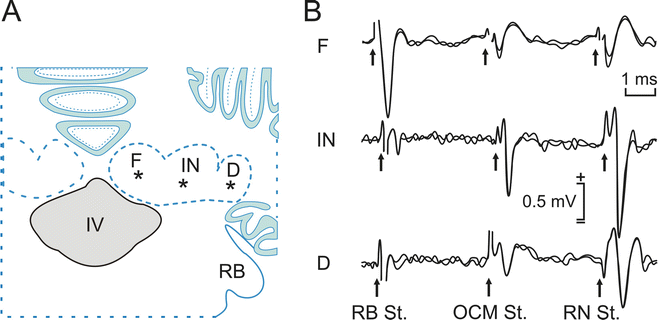

  

  Examples of antidromic field potentials recorded in a behaving cat. (a) A diagram of the recording sites. (b) Antidromic field potentials recorded in fastigial (F), interpositus (IN), and dentate (D) cerebellar nuclei. These field potentials were evoked in behaving cats by electrical stimulation of the contralateral restiform body (RB), oculomotor nucleus (OCM), and red nucleus (RN). Other abbreviations: IV fourth ventricle, St. stimulation

2.3.4 Neuronal Identification

Once the nucleus to be recorded is located, the unitary activity of single neurons of this structure can be recorded and identified. To identify the recorded neuron, it has to be antidromically activated from its projection site, and it has to be checked that the recorded neuron coincides with the activated one. The antidromic activation of a single neuron inside a nucleus involves the production of an action potential in its axon (due to an electrical stimulation) and the recording of an action potential evoked in its soma. The stimulating electrode has to be bipolar to minimize the area stimulated and to avoid the production of artifacts in the recording area. A cathodal stimulus of 50 μs of duration and with an intensity lower than 0.1 mA should be enough if both electrodes (stimulating and recording) are in the right place. The stimulus should be applied at 1 Hz in order to prevent any accumulative effect. Figure 5a, b shows the antidromic activation of a red nucleus neuron from the ipsilateral facial nucleus. Some recordings are superimposed to show the stability of the antidromic activation. The shape of the potentials evoked antidromically can be positive-negative-positive if the recording is made proximal to the axon initial segment and negative-positive if the recording is proximal to the soma or to the main dendrites. Moreover, the shape depends on the macroscopic organization of the surrounding extracellular space. The amplitude of the recorded action potential depends on the characteristics of the electrode and the recording system, as well as on the distance to the plasmatic membrane of the activated neuron (see Note 6).

Fig. 5

Examples of antidromic identification of recorded motoneurons in a behaving rabbit. (a) A diagram of the stimulating (St.) and recording (Rec.) sites. (b) Example of the antidromic activation of a facial motoneuron at threshold intensity (left) and of a spontaneous collision test (right). (c, d) Antidromic activation of abducens motoneurons at high frequency, evoking delayed invasions of the initial segment/somatodendritic compartment (c) or the initial segment compartment (d). (e) Use of the collision test for the antidromic identification of a cerebellar interpositus neuron projecting to the contralateral red nucleus

• 1. The threshold stimulus is the one that produces an antidromic action potential in 50 % of cases. The antidromic potential usually has smaller amplitude and longer duration than the spontaneously (or orthodromically) generated potential. During the antidromic stimulus, it is easy to produce a delay in the invasion of the soma (or inflection in the IS/SD [initial segment/somatodendritic compartments] space) (Fig. 5c). The explanation is that the potential that goes from the initial segment to the soma has to discharge the considerable capacitance of the plasmatic membrane covering the neuronal body from the small current generated in the initial segment. This process needs time, and it can be observed as an inflection in the potential recorded extracellularly. During certain situations (high-frequency stimulation, neuronal lesion, etc.), the antidromic action potential could be unable to invade the somatic compartment (Fig. 5d).

• 2. To determine whether the unitary recording corresponds to a soma or to a passing axon. The action potential recorded in a soma has a different shape to the one recorded at the axonal level. Moreover, a somatic potential can be recorded around 50 μm away, while the distance can be considerably reduced when the recording corresponds to an axon. Finally, an inflection in the IS/SD space can be found in somatic recordings but never in axon recordings.

• 3. To check whether a particular activation is antidromic. Usually, an antidromic action potential is produced with a variation of <0.1 ms in its latency of activation, showing great stability in the velocity of propagation of this action potential through the axon (see Note 7). Frequently, the latency for the antidromic action potential is lower than the latency for the synaptic action potentials evoked by the stimulating electrode. The antidromic activation may be maintained after high-frequency stimulation (see Note 8).

• 4. To identify a unitary recording, it is crucial to determine whether the neuron whose electrical activity is being recorded is the one activated antidromically. In this case, the best procedure is to use the collision test. The electrical stimulus applied to an axon to evoke an antidromic action potential is triggered by a spontaneous action potential. If the stimulus is applied to the axon well after the spontaneous action potential, the two potentials (spontaneous and antidromic) do not coincide in time across the axon, and the antidromic action potential can reach the soma, where it is recorded (Fig. 5e). If the electrical stimulation is applied to the axon time in advance, the antidromic action potential can coincide in its way across the axon with the orthodromic potential, and the two activities will collide. In this case, the propagation of both potentials across the axon will stop, and no antidromic action potential will be recorded in the soma. The minimum interval (I) for this to occur is I(s) = 2T(s) + PR(s), where T is the conduction time through the axon and PR is the refractory period of the same axon. In practice the refractory period changes between 0.8 ms and 4 ms, and the approximate values can be taken as those corresponding to the minimum interval (see Note 9).

2.3.5 Synaptic Effects

With the help of the different electrophysiological techniques described here, the synaptic effects (excitatory and/or inhibitory) of a neuron on its target (muscular fiber and other neurons) can be examined in an alert behaving animal. These synaptic effects can be studied through spike-triggered average techniques or by analyzing the experimentally evoked field postsynaptic potentials.

• 1. The action potential of the neuron can be used as a trigger of the extracellular electrical activity in the area where axons make synapses with their target. This activity should be recorded from 2 ms before to 8 ms after the presentation of the action potential. The recording tools have to be set at a very high resolution in terms of time and voltage. Fig. 6a shows an average obtained from 3000 stimulus presentations with a digital resolution of 20 μV and 5 μs. These recorded signals are usually very small; therefore, the acquisition resolution must be very high.

  Fig. 6

  

  Examples of spike-triggered average recordings. (a) A diagram of the experimental design and an example of a postsynaptic field potential recorded in the abducens (Abd) nucleus and triggered by action potentials recorded in the ipsilateral rostral reticular formation (RF). (b) Extracellular field potentials recorded in the Abd nucleus and triggered by action potentials recorded in the ipsilateral (1) and contralateral (2) RFs and in the contralateral (3) medial vestibular (cMV) nucleus

• 2. In this type of recording, two effects can be easily identified:

  • (i) The action potential arrival evoked by the neuron used as a trigger. This potential should be positive-negative-positive (if the axon of the neuron acting as a trigger continues to other targets) or positive-negative (if the axon of the neuron acting as a trigger ends in the recording target).

  • (ii) The beginning and the shape of the synaptic potential. The beginning of the extracellular synaptic potential has to take place ≈ 0.3 ms after the action potential arrival. The polarity of the potential will be positive if the synapse is inhibitory and negative if it is excitatory.

  • 3. In general, the averaged synaptic potentials have a duration of 2–6 ms, due to the currents generated while postsynaptic membrane channels are open. The shape of the averaged potentials tends to simulate the first or second derivative of the recorded intracellular synaptic potentials. The amplitude of the averaged potential depends on a number of factors: number of activated cells, neuronal density around the recording electrode, density of the synaptic buttons, concentration and kinetics of the postsynaptic ionic channels, ions displaced through their channel, etc.

  • 4. The spike-triggered average technique requires a solid anatomical and structural knowledge. For example, it is important to know whether the synaptic contacts are in the dendrites or in the soma of the neurons. Information regarding the approximate number of neurons activated by the trigger is also useful for the proper interpretation of the evoked synaptic potential (see Note 10). Figure 6b shows three examples of recordings carried out in the abducens nucleus triggered by three different neuronal types with excitatory (neurons 1 and 3) or inhibitory (neuron 2) effects. Differences in amplitude of the recorded potentials are due to different projection areas, to their density, of them, and to the number of innervated neurons.

  • 5. Field postsynaptic potentials can be recorded in certain neuronal areas after stimulating a fascicle of axons projecting to it. If the recording electrode is big enough, it will act as an electric microscope, recording the effects of several postsynaptic potentials in different synapses. The algebraic addition of all these postsynaptic potentials will produce the field postsynaptic potential. The shape (positive or negative), latencies, amplitudes, etc. will follow the same principles as the postsynaptic unitary activity, depending on: (i) type of synapse (excitatory or inhibitory), (ii) neuron structure (dendrites or somas), and (iii) type of recording (intracellular or extracellular) (Fig. 7).

    Fig. 7

    

    Differences in amplitude and profiles of excitatory (top) or inhibitory (bottom) synaptic field potentials recorded intracellularly (left) or extracellularly (right) depending on the location of the synapse and of the recording electrode

  • 6. Field postsynaptic potentials are easy to record in alert behaving animals, and changes in their amplitudes or slopes can be followed during successive recording sessions. Before recording these changes in chronically implanted animals, it is convenient to carry out a depth-profile analysis of field potentials recorded around the selected synapses in acute animals. The aim is to accurately identify the characteristics of the evoked field potentials. This will facilitate the proper identification of the recorded field potentials in the chronic preparation. Figure 8 shows a field potential depth profile carried out through the different hippocampal layers from the CA1 area to the dentate gyrus. Interestingly, the recorded synaptic effects can be distinguished in the evoked postsynaptic potentials depending on whether the stimulation was done in the Schaffer collaterals or in the perforant pathway. Simultaneously, the short-term synaptic effects can be studied by presenting a pair of pulses. Depending upon the selected synapse, the effects of the second stimulus will be larger, smaller, or zero in relation to the effects of the first pulse. For depth-profile analysis, recordings should be carried out in steps of 100 μm. The differences along layers have to be interpreted depending on: (i) type of synapse (excitatory or inhibitory), (ii) neuron structure (dendrites or somas), and (iii) type of recording (intracellular or extracellular).

    Fig. 8

    

    Examples of depth profiles evoked in the hippocampus of a behaving mouse by electrical stimulation (St.) of the ipsilateral CA3 area (i.e., Schaffer collaterals) or the perforant pathway (see Ref. [10] for details)

2.3.6 Relationships between Neural Activities and Behavior

The relevance of this approach is that neural activities can be correlated with some sensorial stimulation, motor responses, the performance of complex behavioral tasks, and, finally, the acquisition of new motor and cognitive abilities.

• 1. In the peristimulus time histogram (PSTH) procedure, the same signal used as sensorial stimulus or a particular moment of a motor response acts as a trigger of the recorded neural activity. Previously, the action potentials should be transformed into square pulses of a given duration (e.g., 1–2 ms). These pulses are accumulated during a given period around the trigger stimulus. For this analysis, the bin size has to be stated as well as the number of times that the test is applied. The obtained responses are considered as the number of action potentials accumulated in each temporal bin (ms). This PSTH procedure can also be applied to experimentally acquired motor responses (Fig. 9).

  Fig. 9

  

  Unitary recordings carried out in the red nucleus of a behaving rabbit during a classical eyeblink conditioning. (a) Experimental setup. (b) Representative recordings of the EMG activity of the orbicularis oculi (OO) muscle and of a red nucleus neuron following paired conditioned stimulus (CS) and unconditioned stimulus (US) presentations. (c, d) Two different types of neuron recorded in the red nucleus during classical eyeblink conditioning of a well-trained rabbit (see Ref. [8] for details)

• 2. The multi-unitary spike-sorting analysis allows discriminating different action potentials from different neurons recorded simultaneously through the same recording electrode. Before correlating the recorded action potentials with sensory, motor, or complex behavioral signals, some mathematical analyses are needed to separate firing activities collected from each neuron.

• 3. A direct way to test synaptic properties is to study the input-output curves at different interstimulus intervals. For example, in the synapses between hippocampal CA3 and CA1 areas, the Schaffer collaterals are stimulated with paired pulses (40 ms of interstimulus interval) at increasing intensities (0.02–0.2 mA). Another test is to determine the effect of paired pulses presented at different (10, 20, 40, 100, 200, and 500 ms) interstimulus intervals when using intensities corresponding to 40 and 60 % of the amount necessary to evoke a saturating response. The pair of pulses is repeated five times with time intervals longer than 30 s, to avoid as much as possible interference with slower short-term potentiation (augmentation) or depression processes. To avoid any cumulative effects, intensities and intervals are presented at random. For the range of intensities suggested here, no population spikes should be observed in the collected recordings.

• 4. Long-term potentiation (LTP) is an experimental approach used to test functional synaptic properties. First, fEPSPs are collected for 15 min to establish a baseline. Pulse intensity is set at 35–45 % of the amount necessary to evoke a maximum field potential response (usually 0.05–0.25 mA)—that is, well below the threshold for evoking a population spike if records are carried out in the hippocampal circuit. After baseline recordings, high-frequency stimulation (HFS) sessions are presented, consisting of five 200 Hz, 100 ms trains of pulses at a rate of 1/s. This protocol is presented six times, at intervals of 1 min. Thus, a total of 600 pulses are presented during an HFS session (see Note 11). After each HFS session, the same stimulus is presented every 20 s for 30 min during the first LTP session and for 15 min on the following days.

• 5. These approaches can be used for correlating neuronal activity with learned responses in control animals but also in genetically manipulated ones. A very popular learning paradigm is the classical eyeblink conditioning using trace or delay paradigms (Fig. 10a, b). This classical conditioning task can be easily used in many species, such as mice, rats, or rabbits. For example, for trace conditioning in mice, a tone (20 ms, 2.4 kHz, 85 dB) is presented as conditioned stimulus (CS). The unconditioned stimulus (US) consists of a 500 μs, 3× threshold, square, cathodal pulse applied in the trigeminal nerve, producing the closure of eyelids. The US starts 500 ms after the end of the CS, and the pairing of the two stimuli evokes conditioned eyelid responses that can be recorded in the EMG activity of the orbicularis oculi muscle (Fig. 10c). A conditioning session consists of 60 CS-US presentations and lasts ≈ 30 min. A total of two habituation, ten conditioning, and five extinction sessions are usually performed for each animal. For habituation and extinction sessions, only the CS is presented. In the same sessions, the local field potential is recorded in some neuronal structures (e.g., the CA1 area of the hippocampus). During the stimulus interval, the fEPSP evoked by stimulating the axons making synapses with the CA1 area (e.g., the Schaffer collaterals) can be recorded. The amplitude and/or slope of the field-evoked postsynaptic potentials can be correlated with the number of conditioned responses through the experimental sessions.

  Fig. 10

  

  Example of learning-dependent changes in synaptic strength evoked by classical eyeblink conditioning of alert mice. (a) Experimental diagram with indication of conditioned stimulus (CS) and unconditioned stimulus (US) presentations. (b) From top to bottom are illustrated conditioning paradigm, the EMG recording of the orbicularis oculi (OO) muscle, and the extracellular activity of the contralateral hippocampal CA1 area. Fig. 10 (continued) A field excitatory postsynaptic potential (fEPSP) was evoked in the CA1 area by electrical stimulation (St.) of ipsilateral Schaffer collaterals. (c) Evolution of fEPSP slopes (top) and of the percentage of conditioned responses (bottom) across habituation (hab.), conditioning, and extinction sessions of conditioned (red triangles and dots) and pseudoconditioned (blue triangles and dots) mice. (d) Differences in fEPSP slopes (top) and in the percentage of conditioned responses between wild-type (dark blue triangles and circles) and knockout (for dopamine D1 receptors; light blue triangles and circles) mice (see details in Refs. [1, 6])

• 6. Recording of the fEPSPs during paired-pulse stimulation, LTP tests, and learning tasks can be used to check functional changes produced after receptor and/or ion channel manipulation in mouse or rat experimental models (Fig. 10d).

• 7. The amount of data that can be obtained with electrophysiological techniques is huge, mainly because multiple recordings can be made simultaneously in different brain areas during different behaviors (innate and acquired). Therefore, this field also requires a thorough training in data analysis and in representation procedures (Fig. 11).

  Fig. 11

  

  Example of changes in functional capabilities of different hippocampal synapses across a classical eyeblink conditioning. (a) Changes in learning-dependent synaptic strength of the nine selected synapses. (b) Evolution of the percentage of conditioned eyelid responses. The corresponding color code is illustrated at the right of (a) and (b) (see Ref. [10] for details)

3 Notes

• 1. Enameled silver wire of 200 μm in diameter is the best option for stimulating electrodes in chronic preparation of large mammals (rabbits and cats). Although silver is toxic in the long term, no damage is seen during the experimental period. The advantage over stainless steel wire is that the latter is too rigid and can act as a knife in the brain during the animal’s movements, including breathing. For small mammals (mice and rats), it is better to use Teflon-coated tungsten wire (25–50 μm). Other wires such as Teflon-coated platinum-iridium or chrome-nickel (25 μm) can also be used but are more expensive.

• 2. If the artifact persists, grounding of the animal and of the recording system has to be checked. As a general condition, all the electrical equipment and the animal preparation have to be carefully connected to the ground system. A simple procedure to prevent polarization of stimulating electrodes is to use very short-lasting (100 μs) positive-negative pulses.

• 3. The same stimulus will activate a myelinated axon faster than a dysmyelinated one. Moreover, applying an excessive current during a repeated stimulation can polarize the electrode and even make an electrolytic lesion in the surrounding tissue. It is always better to use short-lasting pulses of a relatively high intensity than long-lasting ones of a lower intensity.

• 4. In general, the stimulation of a central pathway or a peripheral nerve usually produces a complex potential composed of positive and negative waves. For a proper interpretation of the collected field potential, it is always necessary to have a good understanding of the stimulated neural circuits. It is always helpful to implant the recording electrode as far as possible from the stimulating electrode. This simple procedure can help to record potentials at longer latencies, making it easier to discriminate the different components of the recorded field potential.

• 5. In 1947, Lorente de Nó termed a closed field to be when the electrical current flow goes from the center to the periphery of a nerve structure and vice versa, but no electrical activity can be recorded outside this structure. This means that sources and sinks have a certain symmetric relationship so that currents and potentials are nearly all confined to some local region. Good examples of closed fields are brainstem motor nuclei.

• 6. As already indicated for field potentials, the potential recorded from a single neuron can also decay with distance, following the gradient of approximately 5 μV per μm as the recording electrode moves away from the neuron. The shape of action potentials recorded in the extracellular space corresponds approximately to the second derivative of the action potential recorded intracellularly. The intensity of the electrical stimulation and the exact site for the recording have to be accurately established to activate and to record a single neuron. Action potential s from different neurons can be added linearly and algebraically, a fact that cannot be easily interpreted from the electrophysiological point of view.

• 7. The velocity of an antidromic activation (V) is calculated from the antidromic activation (AA) latency, subtracting the time it takes to produce the action potential at the stimulation site (top), that is around 0.2 ms. Therefore, the conduction time though a given axon (T) is T(s) = AA(s) – top(s). When the distance (d) between the stimulation and the recording sites is known, it will be V (m/s) = d(m)/T(s).

• 8. The maximum frequency that can be applied to a neuron for an antidromic activation depends on its minimum interval, that is, the minimum time between two consecutive stimuli to induce two successive action potentials (Fig. 6b). The minimum interval is different between neurons and ranges from 0.8 to 4 ms for large neurons. These intervals represent frequencies between 200 and 1250 Hz. At these frequencies, it is usually not possible to evoke a synaptic activation. Even when the synaptic activation is accomplished, the action potential generated appears with a large variability (more than 0.2 ms), as opposed to the great stability found in the antidromic activation latency (less than 0.1 ms).

• 9. The collision test is applied online to identify a recorded neuron. New tools have been created to facilitate this identification, although the collision test remains one of the most accurate and, especially, fast tests to apply. Nevertheless, there is no point in taking too much time in identifying the neuron because this can be lost in the process.

• 10. The spike-triggered average technique should be used only with dense projections and with neurons densely assembled in the nucleus. The effect of a projection on distal dendrites, when the number of neurons is scant, or if neurons are dispersed in the recording site, is difficult to study with this technique; that is, the collected extracellular potential would be in the same range as the system (both recording and analysis) noise.

• 11. In order to prevent evoking large population spikes and/or the appearance of local seizures, the stimulus intensity during high-frequency stimulation should be set at the same value as that used for generating baseline recordings. Any animal showing an afterdischarge or a motor seizure following the high-frequency stimulation protocol should be eliminated from the study. These effects can be checked by online electroencephalographic recordings and by visual observation of the stimulated animal.

References

Gruart A, Muñoz MD, Delgado-García JM (2006) Involvement of the CA3-CA1 synapse in the acquisition of associative learning in behaving mice. J Neurosci 26:1077–1087
Madroñal N, Gruart A, Delgado-García JM (2009) Differing presynaptic contribution to LTP and to associative learning in alert behaving mice. Front Behav Neurosci 29:3. doi:10.3389/neuro.08.0072009
Valenzuela-Harrington M, Gruart A, Delgado-García JM (2007) Contribution of NMDA receptor NR2B subunit to synaptic plasticity during associative learning in behaving rats. Eur J Neurosci 25:830–836
Gruart A, Sciarretta C, Valenzuela-Harrington M, Delgado-Garcia JM, Minichiello L (2007) Mutation at the TrkB-PLCγ-docking site affects hippocampal LTP and associative learning in conscious mice. Learn Mem 14:54–62
Fontinha BM, Delgado-García JM, Madroñal N, Sebastião AM, Gruart A (2009) Adenosine A2A receptor modulation of hippocampal CA3-CA1 synapse plasticity during associative learning in behaving mice. Neuropsychopharmacology 34:1865–1874
Ortiz O, Delgado-García JM, Espadas I, Bahí A, Trullas R, Dreyer JL, Gruart A, Moratalla R (2010) Associative learning and CA3-CA1 synaptic plasticity are impaired in D1R Null, Drd1a −/− mice and in hippocampal siRNA silenced Drd1a mice. J Neurosci 30:12288–12300
Trigo JA, Gruart A, Delgado-García JM (1999) Discharge profiles of abducens, accessory abducens and orbicularis oculi motoneurons during reflex and conditioned blinks in alert cats. J Neurophysiol 81:1666–1684
Pacheco-Calderón R, Carretero-Guillén A, Delgado-García JM, Gruart A (2012) Red nucleus neurons actively contribute to the acquisition of classically conditioned eyelid responses in rabbits. J Neurosci 32:12129–12143
Leal-Campanario R, Delgado-García JN, Gruart A (2013) The rostral medial prefrontal cortex regulates the expression of conditioned eyelid responses in behaving rabbits. J Neurosci 33:4378–4386
Gruart A, Sánchez-Campusano R, Fernández-Guizán A, Delgado-García JM (2015) A differential and timed contribution of identified hippocampal synapses to associative learning in mice. Cereb Cortex. 25(9):2542–2555. doi:10.1093/cercor/bhu054
Acknowledgments
This work was supported by the grants BFU2011-29286 from the Spanish Ministry of Economy and Innovation and by the Excellence Program of the Junta de Andalucía. We are grateful to the technicians who have collaborated in the past few years to improve the electrophysiological in vivo recording and stimulating techniques used in our laboratory: José Antonio Santos-Naharro, María Esteban-Masferrer, Noelia Rodríguez-García, José María González-Martín, and María Sánchez-Enciso.
Author information
Authors and Affiliations
Corresponding author
Editor information
Editors and Affiliations
Rights and permissions
Copyright information
© 2016 Springer Science+Business Media New York
About this protocol
Cite this protocol
Gruart, A., Delgado-García, J.M. (2016). Electrophysiological Recordings in Behaving Animals. In: Luján, R., Ciruela, F. (eds) Receptor and Ion Channel Detection in the Brain. Neuromethods, vol 110. Humana Press, New York, NY. https://doi.org/10.1007/978-1-4939-3064-7_23
Download citation
DOI: https://doi.org/10.1007/978-1-4939-3064-7_23
Publisher Name: Humana Press, New York, NY
Print ISBN: 978-1-4939-3063-0
Online ISBN: 978-1-4939-3064-7
eBook Packages: Springer Protocols