Nondestructive Visualization Using Electromagnetic Waves for Real and Practical Sensing Technology for Robotics

Abstract

This section describes novel methods of electromagnetic wave nondestructive visualization (NDV) for assessing qualification and durability of concrete and wooden structures, which involves devices, systems, and image processing. As the first, the basic knowledge and principles on dielectric properties of materials, wave propagation in media involving plane waves in vacuum and in non-conducting and non-magnetic dielectric media were introduced. As the second, the dielectric properties of concrete and NDV techniques for concrete structures were introduced. After the introduction of conventional methods to detect internal cracks in concrete structures, a novel development of a millimeter wave scanner for NDV of concrete was introduced where the performance of the scanner to detect surface cracks covered by other sheet materials was discussed. Miscellaneous image processing techniques to recognize the target using pattern recognition methods were also introduced. Wood is a material made of the plant cells of trees. Wood shows anisotropy in physical and mechanical properties, such as elastic moduli, strength, and dielectric constants. In addition, wood is deteriorated by biological agents such as insects and fungi, and these deterioration often generate in inner or hidden areas of wood and wooden construction. The deterioration is closely associated with moisture content of wood. In this section, the feasibility of technologies using electromagnetic waves for the nondestructive evaluation of properties and deterioration of wood and wooden construction, is introduced. The reaction of wood to electromagnetic wave such as transmission and reflection of millimeter wave through and from wood was discussed. The development of wooden wall scanner for nondestructive diagnoses of wooden houses using FMCW radar was introduced.

1 General Introduction

Imaging techniques for investigating physically inaccessible objects have been topics of research for many years and have found widespread applications in the field of nondestructive visualization (NDV). All electromagnetic wave methods in NDV involve Maxwell’s equations and cover a broad range of the electromagnetic spectrum, from static or direct current to high frequencies, e.g., X-ray and gamma ray methods. Imaging science is concerned with the formation, collection, duplication, analysis, modification, and visualization of images. Electromagnetic NDV is essential for detecting anomalies or defects in both conducting and dielectric materials by generating two-dimensional or three-dimensional image data based on the electromagnetic wave principles. For forward imaging approaches, the excitation transducers usually couple the electromagnetic energy to the test objects, while the receiving sensors measure the response of energy/material interaction. Depending on different energy types and/or levels, various electromagnetic sensors/transducers can be used for a broad range of applications, e.g., microwave imaging and millimeter wave imaging. After acquiring and storing the electromagnetic images, those data are passed through the inversion-techniques block, which involves object reconstruction, pattern recognition, etc. Electromagnetic wave NDV has been attracting much attention in applications for the evaluation of concrete and wood structures, e.g., buildings, bridges, and houses. Concrete and wood consist of many dielectric components, which provide complexly electromagnetic responses of transparency, reflection, refraction, and scattering. This section describes novel methods of electromagnetic wave NDV for assessing qualification and durability of concrete and wood structures, which involves devices, systems, and image processing.

2 Basic Principles

The foundations of nondestructive visualization (NDV) using electromagnetic (EM) waves lie in EM theory, and the history of this field spans more than two centuries, which is based on the subject of numerous texts such as those by Jackson [1] and Smythe [2]. This overview outlines the basic building blocks, especially concrete, needed to work quantitatively with NDV using EM waves.

Maxell’s equations mathematically describe the physics of EM fields, while constitutive relationships quantify material properties. Combining the two provides the foundations for quantitatively describing EM wave signals.

2.1 Dielectric Properties of Materials

A dielectric material conducts EM waves and is commonly referred to as an insulator. The transition from insulator, which is characterized by low electric conductivity, to conductor, which has high conductivity, is gradual without any clear cutoff point, and many existing materials exhibit both properties. If the conductivity of a material is high, it attenuates EM waves to a larger extent, resulting in a lower penetration depth. The two significant properties of a dielectric material are the real and imaginary parts of its complex dielectric permittivity. The real part is associated with the phase velocity, and the imaginary part signifies the conductivity or attenuation of EM waves in the medium. Dielectric permittivity is often referred to as the dielectric “constant.” This term is misleading, since this property of a dielectric material varies due to several factors. Bell et al. [3] provided some insight into these variations through underlying molecular and atomic mechanisms associated with dielectric constant and conductivity of such materials. A dielectric material increases the storage capacity of a capacitor by neutralizing charges at the electrode surfaces. This neutralization can be imagined to be the result of the orientation or creation of dipoles opposing the applied field. Such a polarization is proportional to the polarizability of the dielectric material, that is, the ease with which it can be polarized. Polarizability is defined as the average induced polarization per unit field strength. The greater the polarizability of a material, the greater will be its dielectric constant. There are four recognized mechanisms of polarization: (a) electronic, (b) atomic, (c) orientation, and (d) space charge or interfacial. The first three polarization mechanisms are forms of the dipole polarization previously mentioned.

They result from the presence of permanent dipoles or from dipoles induced by external fields. The fourth type—space charge polarization—results from charge carriers that are usually present and more or less free to move through the dielectric. When such carriers are impeded in their movement and become trapped in the material or at interfaces, space charge concentrations result in a field distortion that increases the capacitance. The above discussions indicate that the dielectric constant of a material is not such a constant, but is a function of polarizability, which is in turn a function of frequency, temperature, local fields, applied field strength, availability and freedom of charge carriers within the dielectric, and local field distortions. Dielectric conductivity is also affected by the same factors. This is because dielectric conductivity is a function not only of ohmic conductivity but also of the power consumed in polarizing the material. In addition to the “intrinsic loss” caused by the conduction process, there could also be “scattering loss” due to the presence of inhomogeneities within the medium. Since the aggregate particle size is much smaller than the EM wavelength considered at a microwave range, the inhomogeneities in concrete are not likely to cause significant scattering losses. However, this is not true for inhomogeneities with large dimension (e.g., delaminations) and large conductivity (e.g., rebar) or with application at the millimeter wave (MMW) range. These inhomogeneities will be modeled separately, and their effect will be taken into account for the purpose of waveform synthesis.

2.2 Wave Propagation in Media

One of the most important consequences of Maxwell’s equations is the equations for EM wave propagation in a linear medium. In the absence of free charge and current densities, Maxwell’s equations are

$$\begin{aligned} {\nabla } \cdot D & = 0 \\ {\nabla } \times H & = \frac{{{\partial }D}}{{{\partial }t}} \\ {\nabla } \cdot B & = 0 \\ {\nabla } \times E & = \frac{{{\partial }B}}{{{\partial }t}} \\ \end{aligned}$$

(14.1)

The wave equations are derived by taking the curl of

$$\begin{aligned} {\nabla } \times {\nabla } \times E & = - {\nabla } \times \frac{{{\partial }B}}{{{\partial }t}} \\ {\nabla } \times {\nabla } \times H & = - \nabla \times \frac{{{\partial }D}}{{{\partial }t}} \\ \end{aligned}$$

(14.2)

For uniform isotropic linear media, we have D = εE and B = μH, where ε and μ are in general complex functions of frequency ω. Then, we obtain

$$\begin{aligned} {\nabla } \times {\nabla } \times E & = - \varepsilon \mu \frac{{{\partial }^{2} E}}{{{\partial }t^{2} }} \\ {\nabla } \times {\nabla } \times B & = - \varepsilon \mu \frac{{{\partial }^{2} B}}{{{\partial }t^{2} }} \\ \end{aligned}$$

(14.3)

Since ${\nabla } \times {\nabla } \times E = {\nabla }\left( {{\nabla } \cdot E} \right) - \nabla^{2} E = - {\nabla }^{2} E$ and, similarly, ${\nabla } \times {\nabla } \times B = - {\nabla }^{\text{2}} B$,

$$\begin{aligned} {\nabla }^{2} E & = \varepsilon \mu \frac{{{\partial }^{2} E}}{{{\partial }t^{2} }} \\ {\nabla }^{2} B & = \varepsilon \mu \frac{{{\partial }^{2} B}}{{{\partial }t^{2} }} \\ \end{aligned}$$

(14.4)

Monochromatic waves may be described as waves that are characterized by a single frequency. Assuming the fields with harmonic time dependence ${\text{e}}^{ - i\omega t} ,$ so that $E\left( {x,t} \right) = E(x){\text{e}}^{ - i\omega t}$ and $B\left( {x,t} \right) = B(x){\text{e}}^{ - i\omega t} ,$ we obtain the Helmholtz wave equations

$$\begin{aligned} {\nabla }^{2} E + \varepsilon \mu \omega^{2} E & = 0 \\ {\nabla }^{2} B + \varepsilon \mu \omega^{2} B & = 0 \\ \end{aligned}$$

(14.5)

Plane waves in vacuum

Suppose the medium is vacuum, so that $\varepsilon = \varepsilon_{0}$ and $\mu = \mu_{0}$. Furthermore, suppose E(x) varies in only one dimension. Then, Eq. 14.5 becomes

$$\frac{{{\text{d}}^{2} E(z)}}{{{\text{d}}z^{2} }} + k^{2} E(z) = 0$$

(14.6)

where the wave number k = ω/c. This equation is mathematically the same as the harmonic oscillator equation and has solutions. Therefore, the full solution is

$$E_{k} \left( {z,t} \right) = \alpha {\text{e}}^{{ \pm ikz - i\omega\;t}} = \alpha {\text{e}}^{{ - i\upomega(t \mp \frac{z}{c})}}$$

(14.7)

where α is a constant vector.

This represents a sinusoidal wave traveling to the right or left in the z-direction at the speed of light. Using the Fourier superposition theorem, we can construct a general solution of the form

$$E\left( {z,t} \right) = A\left( {z - ct} \right) + B(z + ct)$$

(14.8)

Plane waves in non-conducting, non-magnetic dielectric

In a non-magnetic dielectric, we have $\mu = \mu_{0}$ and the index of refraction

$$n\left( \omega \right) = \sqrt {\frac{\varepsilon (\omega )}{{\varepsilon_{0} }}}$$

(14.9)

The results are the same as in vacuum, except that the velocity of wave propagation or the phase velocity is now $v = c/n$ instead of c. Then, the wave number is

$$k\left( \omega \right) = n(\omega )\frac{\omega }{c}$$

(14.10)

3 NDV for Diagnosis of Concrete Structures

This section reviews some NDVs for diagnosis of concrete structures and introduces MMW imaging technology for detecting submillimeter-wide cracks under a bill-posting prevention sheet on a concrete telegraph pole.s

3.1 Degradation Phenomenon of Concrete Structures

In the social environment based on concrete structures, the maintenance and renewal of aging infrastructure is becoming a major issue. Operating such aged facilities efficiently and safely requires the following maintenance cycle: design, inspection, diagnosis, evaluation, and implementation of countermeasures. To assure the safety of facilities, it is necessary to ascertain their state to a high degree of accuracy and detail. Moreover, among the steps in the maintenance cycle, the inspection and diagnosis processes are extremely important. At present, the usual way to inspect and diagnose facilities with high precision is to perform strength testing and material analysis on samples removed from an existing facility. This method, by definition, consumes part of an existing facility, so it is difficult to apply it to the entire structure of an aged existing facility. Furthermore, in large-scale facilities like tunnels, the conditions often vary with the measurement position, so it is difficult to evaluate the condition of the whole facility from local measurements. On the other hand, non destructive testing evaluates the condition of a structure without damaging it, so it has two advantages: it can be applied to the whole of a large-scale structure and can efficiently evaluate the degradation condition of that structure. The ideal situation and the actual state of the maintenance of steel-reinforced concrete structures are shown schematically in Fig. 14.1 [4] using the analogy between the degradation process of steel-reinforced concrete and the progress of a disease in humans. In the case of a human disease, if the disease can be detected in its latent phase (i.e., its premorbid phase) by regular health checks, it can be prevented from reaching an acute state, so major surgery is unnecessary. Likewise, in the case of concrete structures, it is important to take effective action at the stage before visible degradation of the concrete occurs. If high precision facility evaluation by non-destructive testing were available, it would be possible to continue operating and maintaining existing facilities for a long time.

Fig. 14.1

The ideal situation and the actual state of the maintenance of steel-reinforced concrete structures

3.2 NDV Techniques for Concrete Structures

Methods for seeing through the covering material to observe the condition of the surface beneath it are classified by the physical phenomena that are used. In particular, methods that use X-rays, ultrasonic waves, or microwaves have been applied in various fields. Table 14.1 lists the series of NDV techniques for each target of concrete structures, as shown in Fig. 14.2.

Table 14.1 Evaluation methods and NDT for reinforced concrete structures

Fig. 14.2

Evaluation methods and NDT for reinforced concrete structures. a. Structure dimension b. Deterioration situation

X-rays are a form of ionizing radiation that have high transmittance for materials other than water and heavy metals and allow imaging with micrometer-order spatial resolution. They are applied for medical purposes such as 3D imaging of internal organs and bones, but since they are harmful to humans, exposure levels must be carefully controlled: This would be a safety problem for workers using X-rays inspecting multiple concrete poles every day. Another problem is that practical X-ray imaging equipment is based on transmission, so it should really have a separate transmitter and receiver; however, for work sites with limited work space, reflection-based imaging equipment can be used.

Ultrasonic waves are elastic waves that have almost no effect on the human body and have high transmittance and millimeter-order spatial resolution for reflection-based imaging. They are therefore used for medical three-dimensional (3D) imaging of fetuses, but the procedure requires the application of grease between the ultrasonic wave transceiver and object to be observed for efficient sound wave transmission. The expense of applying and removing grease would be a problem for inspection of a huge number of poles.

Microwaves are EM waves that have high transmittance and centimeter-order spatial resolution inside concrete, so they are used to inspect rebar. However, this technique does not provide the submillimeter-order spatial resolution required for crack detection, so imaging performance remains a problem.

3.2.1 Conventional Electromagnetic Wave Techniques for Internal Checking

The continued deterioration of concrete structures, such as buildings, bridges, tunnels, and highways, increases the danger of their collapse. The durability of concrete structures can be estimated from the position, number, and diameter of their reinforcing bars. The distance from the surface of the structure to a reinforcing bar is a particularly important parameter for estimating the bar’s corrosion state. Pulse radar, which makes a two-dimensional (2D) azimuth–range image, has attracted much attention for nondestructively checking the positions of reinforcing bars because of its simple operation [5]. However, a conventional pulse radar system cannot measure the positions of shallow bars due to its low depth resolution of several tens of millimeters defined from its nanosecond-order pulse width. The measurement of the shallow position is becoming important because the shallow bar is easily corroded.

An ultra-wideband (UWB) antenna is an attractive solution to improve the depth resolution because of its wide bandwidth corresponding to the pulse width of a few hundred ps [6–10]. However, conventional UWB antennas are not suited for measuring the bar’s position in reinforced concrete structures because of its omnidirectional radiation which induces multipath reflected pulse waves as a noise signal. This has led to the development of tapered slot antennas (TSAs), which are directional UWB antennas with a directivity of over 6 dBi [11–20]. The TSAs usually have isotropic radiation characteristics in the E- and H-planes, which evenly illuminate the target. However, the isotropic radiation characteristics are inefficient regarding the illumination power for a synthetic aperture radar (SAR) technique which is a post signal processing technique used to improve the resolution of the radar image. This technique uses the correlation between the acquired 2D data along the azimuth axis. The spatial resolution of the SAR image improves the signal-to-noise ratio (SNR), resulting in a higher contrast image. The SAR technique requires a wide illuminated area in the H-plane and a narrow one in the E-plane of the antenna because the correlation is performed only for the H-plane data. Therefore, we developed a TSA with orthogonally anisotropic directivity, that is, wide and narrow radiation patterns in the H- and E-planes, respectively.

The aim of our study was to develop an SAR system with high spatial resolution for the nondestructive evaluation of reinforced concrete structures. We numerically and experimentally investigated a new antenna suitable for a SAR system using an ultra-short pulse. Testing of a prototype system demonstrated that it can detect the bars in reinforced concrete samples.

Mochizuki optimized the shape of a Vivaldi tapered slot antenna (VTSA) by using a commercially available numerical simulator [21]. Using this simulator makes it easy to evaluate EM fields (both near and far) from an antenna and its S-parameters.

Figure 14.3 illustrates the configuration of our developed antenna, which is an anisotropic directional antenna (a VTSA with substrate cutting and corrugation). It is fabricated on a substrate with a relative dielectric constant of 3.75, a loss tangent of 0.02, and a thickness of 1.0 mm including the thin copper coating. It consists of three parts: a coaxial-to-coplanar waveguide (CPW) transition, a CPW-to-slotline transition, and a tapered slotline. It has a uniquely shaped substrate below the slotline, which is formed by substrate cutting. This shape produces the difference in radiation patterns in the E- and H-planes (which are defined by the xz and yz planes, respectively). Corrugation is used on both sides of the tapered slotline to reduce sidelobe levels. Mochizuki computed the radiation patterns in the E- and H-planes of the developed antenna as well as those of an isotropic directional antenna (VTSA without substrate cutting and corrugation). Figure 14.4 shows their radiation patterns at 10 GHz. The developed antenna has a narrower beam width for the E-plane and a wider beam width for the H-plane than the isotropic directional antenna. The ratio of the 10-dB beam width of the H-plane to that of the E-plane for the developed antenna is 120:60 (2:1), which is higher than that for other TSAs. This difference in the radiation patterns is mainly due to removing the substrate below the tapered slotline. The EM energy flowing from the feed point to the aperture of the TSA is highly concentrated in the substrate below the tapered slotline. When the substrate below the slotline is removed, the energy spreads in the direction of the H-plane; it cannot spread in that of the E-plane due to the limited slotline width. Calculation of the antenna gain shows that the corrugation and substrate cutting increased the gain from 4.7 to 7.6 dBi.

Fig. 14.3

Anisotropic directional antenna

Fig. 14.4

Radiation patterns of anisotropic directional antenna (solid line) and VTSA without substrate cutting and corrugation (dotted line) in E-plane (a) and H-plane (b)

The return loss (S11) of the developed antenna, shown in Fig. 14.3, was measured with a vector network analyzer in free space, and the results are shown in Fig. 14.5. It was found that this antenna works well at a higher frequency than 3.2 GHz.

Fig. 14.5

Return loss (S11) of anisotropic directional antenna

A pulse transmission test in free space (distance of 150 mm) between two of the developed antennas was conducted. The transmitting antenna was driven with a Gaussian pulse with a pulse width of 100 ps. The waveform of the received pulse in the time domain was measured with a high-speed digital sampling oscilloscope. The results, shown in Fig. 14.6, reveal a monocycle pulse wave with a width of 200 ps, which corresponds to a bandwidth of over an octave or more.

Fig. 14.6

Time-domain waveform transmitted with anisotropic directional antennas in free space at the distance between antennas was 150 mm

The SAR imaging system we developed is based on a bistatic pulse radar and uses two of the developed anisotropic directional antennas, as shown in Fig. 14.7. Sinusoidal input for the comb generator is supplied from a signal generator through the amplifier. A pulse with a width of 100 ps is generated and radiated through the transmitting antenna to the target. The backscattered pulse from the target is obtained in the time domain with a high-speed digital sampling oscilloscope through the receiving antenna.

Fig. 14.7

Pulse radar system

The setup used for testing the SAR system is shown in Fig. 14.8. The azimuth and range axes were parallel to the scan and pulse radiation directions, respectively. The elevation axis was normal to the azimuth and range axes. The H- and E-planes of the antennas corresponded to the azimuth range and elevation range planes, respectively, so the illuminated area was elliptical with the major axis parallel to the azimuth axis, as shown in Fig. 14.9.

Fig. 14.8

Experimental setup for SAR imaging

Fig. 14.9

Radar image of reinforced concrete sample

The testing was done using a reinforced concrete sample with two reinforcing bars. As shown in Fig. 14.10, one bar had a radius of 10 mm and the other had a radius of 12 mm. They were set 13 and 11 mm deep, respectively, too shallow to be detected with a conventional imaging system because of its poor resolution (more than 25 mm).

Fig. 14.10

SAR image of reinforced concrete sample

The transmitter illuminated the sample with a pulse wave, and the receiver recorded the backscattered pulse. This process was performed repeatedly and continuously, while the system was moved over the sample. After the sample had been scanned, a 2D radar image corresponding to the azimuth range plane was displayed on a personal computer (PC).

An SAR image, which is an image with higher spatial resolution than the radar image, was also obtained by performing SAR signal processing on the personal computer. This SAR system uses a conventional SAR imaging technique based on the delay-and-sum approach, which collects the backscattered data with a curved profile at a point in the radar image. The number of collected data points for a curved profile was 400, and the relative permittivity of the sample was assumed to be 9.

3.3 Millimeter Wave Scanner for NDV

3.3.1 Features in Millimeter Wave Technologies

To overcome the issues of safety, economy, and imaging performance, we took up the difficult R&D challenge of using MMWs, which are EM waves of higher frequencies than micrometer waves, to develop improved imaging technology. The MMW band includes frequencies from 30 to 300 GHz, but the frequencies specified by the radio law for radar use (imaging is also one use of radar) range only from 76 to 77 GHz (the band allocated to MMW radar). The allocation of MMW radar band frequencies for inspection purposes is being studied. The main concerns in developing MMW radar technology for detecting cracks in CP under bill-posting prevention sheets are (1) the transmittance of the plastic sheet, (2) submillimeter spatial resolution, and (3) ease of equipment operation.

In the band allocated for MMW radar, the relative permittivity of polyvinyl chloride is about 3 and the dielectric tangent is about 0.01, so if Oka and Togo assume a planar wave incident on a 4-mm-thick infinite plane, the attenuation due to reflection and propagation loss is low, about −10 dB, so transmittance is not a significant problem for equipment design. There is concern, however, that the texture of the bill-posting prevention sheet may have a greater effect on attenuation than the sheet’s material properties because of wave scattering at the surface.

Another factor is that the width of the cracks to be detected is less than 1/10 the wavelength of the band allocated to MMW radar, so considering the radar cross-sectional area, the backscattering will be less than −30 dB relative to the power irradiating the surface. On the basis of the above estimates, we are investigating an equipment design in which the irradiation power of the MMW radiation is set to −50 dB to pass through the bill-posting prevention sheet to reach the crack and then pass back through the sheet as backscattering.

Because the minimum beam diameter obtainable by focusing with a quasi-optical system using a lens is limited by diffraction, the beam width is limited to approximately the wavelength. The spatial resolution is therefore about half the wavelength, which means that it is difficult to detect submillimeter-wide cracks using the approximately 4-mm wavelength of the band allocated to MMW radar. For this reason, we have been trying to improve the spatial resolution by detecting near-field scattering. The concept, as shown in Fig. 14.11, is that spatial resolution can be improved because the waves scattered from the crack, which can be regarded as a minute point in a cross section that includes the crack width direction and crack depth direction, are spherical waves. The dispersion of the scattered waves is thus small in the near field. Detecting near-field scattering with submillimeter-order spatial resolution requires the use of an antenna whose aperture is equivalent to the width of the scattered waves at the detection height. Oka and Togo are therefore investigating aperture design at the antenna placement height with consideration given to operability.

Fig. 14.11

Dispersion of wave scattering from a crack

Inspecting all the concrete telegraph poles in the entire country for structural integrity requires highly efficient work. The shortest imaging time could be achieved by covering the entire bill-posting prevention sheet with the antenna for detecting near-field scattering that is needed in the detection of submillimeter-wide cracks, but it is difficult to arrange antenna elements at submillimeter intervals in the crack width direction. Even if the elements are arranged at millimeter intervals, since the bill-posting prevention sheet is about 1.5 m long in the vertical direction, the number of antenna and MMW transmitter and receiver components would be huge and the equipment cost would be uneconomical. The equipment would also be large, which would reduce its portability. To maintain economy and portability, we considered a method in which ten antennas are arranged in a one-dimensional (1D) array in the crack length direction and the array is scanned in the crack width direction. Spatial resolution in the crack width direction is maintained by detecting scattered waves at submillimeter intervals. The equipment can perform multiple scans in the crack length direction to image the entire surface.

3.3.2 Application of Millimeter Wave Scanner

Nippon Telegraph and Telephone Corporation (NTT) in Japan expends much effort in the long-term maintenance and management of the communication network to provide safe and secure communication services to customers throughout the country. Concrete telegraph poles, which are perhaps the most familiar of those facilities to most of us, are susceptible to physical damage, so a high degree of structural integrity is required. Concrete poles and other structures degrade over time; therefore, integrity maintenance requires periodic inspections so that degraded structures can be repaired. Since NTT owns more than ten million CP, such inspection is a daily job for a large number of employees.

Concrete poles carry cables, transformers, and other equipment, which produce an unbalanced load on the structure over many years. The resulting bending stress produces fatigue cracking on the pole surface. When such cracking penetrates as far as the rebar inside the pole, rainwater may enter and cause corrosion that can lead to the rebar breaking. Steel rebar, which is strong in tension, is vital to balance the concrete, which is strong in compression but weak in tension, so broken rebar reduces the integrity of a CP. Considering this degradation mechanism, we focused on the initial stage of degradation, which is the appearance of cracks on the concrete surface. NTT has experimentally verified that submillimeter-wide surface cracks have a high probability of reaching the rebar, so early discovery of the initial degradation is considered to be the best approach to structural integrity maintenance. Therefore, careful visual inspection of the pole surface is performed.

The NTT Access System Laboratories is developing a new technique to replace human visual inspection by using software to automatically detect cracks from images acquired with a digital camera. More details of this technique are given in the Feature Article “Detection of Cracks in Concrete Structures from Digital Camera Images,” in this issue [22].

To prevent unauthorized posting of advertisements on CPs, 2-mm-thick sheets of textured polyvinyl chloride (bill-posting prevention sheets) are bonded to the poles with acrylic resin in the region within hand reach (Fig. 14.12). Exposing the covered surface for visual inspection would require significant work to strip off the sheet and then replace it with a new one after inspection. Since that would not be economically feasible, Oka and Togo conducted research and development (R&D) of a nondestructive inspection technique that allows observation of the pole surface condition without the need to remove the bill-posting prevention sheet [23].

Fig. 14.12

Bill-posting prevention sheet on a concrete pole

On the basis of the design policy described above, we constructed a portable device called CP scan for detecting cracks in CPs under bill-posting prevention sheets (Fig. 14.13). Sixteen intensity phase detection modules having tapered slot antennas are arranged in a 1D array. A signal from the module is input to the baseband circuit at submillimeter scanning intervals in sync with a signal from an encoder attached to the wheels of the unit: In this way, the condition of the CP surface is imaged. The case containing the module, encoder, and baseband circuit weighs less than 4.1 kg and can be held in one hand for scanning. The entire system, including the power supply and PC, weighs less than 10 kg and can be carried by a single person. The 16 modules can image an 8-cm-wide path in a single scan, and one or two workers can inspect a pole in about three minutes by making five or six scans to image the entire region of the bill-posting prevention sheet (Fig. 14.14).

Fig. 14.13

CP scan equipment

Fig. 14.14

Schematic illustration of CP scan in use

3.3.3 Surface Crack Detection with Millimeter Wave Scanner, Crack Scan

To test the practicality of CP scan, a bill-posting prevention sheet was attached to a CP that had been removed for renovation (Fig. 14.15) and CP scan was used to inspect this area. The pole had cracks ranging in width from 0.3 to 0.15 mm. Although this preliminary experiment was suitable for confirming the method’s principle, the attached bill-posting prevention sheet was not bonded to the pole. The scanning rate was 120 mm/s with data being acquired at intervals of 0.2 mm in the scanning direction. That rate will allow one CP to be inspected in about three minutes. A millimeter wave image was obtained after three scans (Fig. 14.16). Although the equipment must be calibrated, the imaging only requires the equipment to be kept tightly against the pole during the scan, so the operation is simple.

Fig. 14.15

Experimental setup

Fig. 14.16

Results of crack detection in test specimen

To allow a single person to perform the inspection, as shown in Fig. 14.16, the power supply and PC components of the system must be small and light, and image processing is essential for automatic crack detection from the acquired images. Therefore, NTT Access System Laboratories is currently developing an algorithm suitable for MMW image analysis.

These experiments used the Crack Scan automatic crack detection software that was subjected to hard disclosure commissioning to AIREC Engineering Corporation in 2008 for evaluation of detection characteristics. The red line in the bottom image of Fig. 14.17 indicates cracks detected from the Crack Scan automatic detection algorithm, confirming that 0.15-mm-wide cracks can be detected. These results open up the prospect of developing portable equipment that can detect cracks that are at least 0.15 mm wide with a scanning time of about three minutes per pole.

3.3.4 Image Reconstruction for Crack Scan

To improve the spatial resolution in the radiative near-field region, Kojima and Mochizuki applied signal processing based on a holographic technique to MMW near-field imaging. A basic holographic algorithm has been proposed to detect concealed weapons and demonstrated a high-resolution 2D image reconstructed with the near-field data measured over the surface of a target at a single frequency [24]. With this technique, it is assumed with the image reconstruction algorithm that near-field waves radiating from the antenna and backscattering from the target point are closely approximated by a spherical wave and that a small-aperture antenna is suitable for radiating the spherical wave. In practical measurement, however, a directivity antenna such as a horn antenna and open-ended oversized waveguide probe are used to obtain high radiation efficiency. With the image reconstruction algorithm, the difference between the near-field radiation pattern of the antenna in the measurement and assumption causes degradation of the spatial resolution of images.

To overcome this issue, we developed an image reconstruction algorithm for improving the spatial resolution of MMW images. Our algorithm is based on deconvolution processing with the near-field radiation pattern from the antenna. We now describe the basic concept of our algorithm and present the reconstruction results from images of a 0.1-mm-wide crack on the surface of a concrete block measured at 76.5 GHz.

The configuration of the measurement model for verifying our algorithm is shown in Fig. 14.17. With our algorithm, the propagation equation should be well described, including the contribution of the near-field radiation pattern. The response of the transceiver, $u_{s} \left( {r^{{\prime }} } \right),$ can be written as a superposition of the response from all positions on the object, taking the effect of the antenna aperture into account:

$$u_{s} \left( {r'} \right) = \mathop {\iint }\limits_{\text{aper}} A\left( {r_{\text{ap}} } \right)\mathop {\iint }\nolimits u_{i} \left( {r - r^{{\prime }} } \right)f\left( r \right)g\left( {r_{\text{ap}} + r^{{\prime }} - r} \right){\text{d}} x\,{\text{d}} y\,{\text{d}}S_{\text{ap}}$$

(14.11)

where f(r) is the object function indicating the dielectric distribution on the surface of the object, $g\left( {r_{\text{ap}} + r^{{\prime }} - r} \right)$ is Green’s function, which is written in three dimensions as

$$g\left( {r_{\text{ap}} + r^{{\prime }} - r} \right) = \frac{{{\text{e}}^{{ - ik\left| {r_{\text{ap}} + r^{{\prime }} - r} \right|}} }}{{\left| {r_{\text{ap}} + r^{{\prime }} - r} \right|}} ,$$

(14.12)

and $u_{i} \left( {r - r^{{\prime }} } \right)$ is the incident electric field at the object surface:

$$u_{i} \left( {r - r^{{\prime }} } \right) = \mathop {\iint }\limits_{\text{aper}} A\left( {r_{\text{ap}} } \right)\frac{{{\text{e}}^{{ - ik\left| {r - (r_{\text{ap}} + r^{{\prime }} )} \right|}} }}{{\left| {r - (r_{\text{ap}} + r^{{\prime }} )} \right|}}{\text{d}}S_{\text{ap}} .$$

(14.13)

Fig. 14.17

(a) Position of the object, the center of the antenna aperture, and (b) antenna aperture in xyz coordinates

Focusing attention on the near-field radiation in Eq. (14.11), we can change the order of the integral equation:

$$u_{s} \left( {r^{{\prime }} } \right) = \mathop {\iint }\nolimits u_{i} \left( {r - r^{{\prime }} } \right)f\left( r \right)\mathop {\iint }\limits_{\text{aper}} A\left( {r_{\text{ap}} } \right)g\left( {r_{\text{ap}} + r^{{\prime }} - r} \right){\text{d}}S_{\text{ap}}\,{\text{d}}x\,{\text{d}}y.$$

(14.14)

By using Eq. (14.3) and the condition $g\left( {r_{\text{ap}} + r^{{\prime }} - r} \right) = g\left( {r - (r_{\text{ap}} + r^{{\prime }} )} \right)$, Eq. (14.14) can be simplified as follows:

$$u_{s} \left( {r^{{\prime }} } \right) = \iint f\left( r \right)\left[ {u_{i} \left( {r - r^{{\prime }} } \right)} \right]^{2} {\text{d}}x{\text{d}}y.$$

(14.15)

Thus, $u_{s} \left( {r^{{\prime }} } \right)$ is written as a convolution integral of f(r) and the square of u_i(r). We can solve the object function f(r) by applying a 2D Fourier transform to both sides of Eq. (14.15):

$$FT_{2D} \left[ {u_{\text{s}} \left( {r^{{\prime }} } \right)} \right] = FT_{2D} \left\{ {\left[ {u_{i} \left( r \right)} \right]^{2} } \right\}FT_{2D} \left[ {f\left( r \right)} \right],$$

(14.16)

where FT_2D indicates the 2D Fourier transform. Thus,

$$f\left( r \right) = FT_{2D}^{ - 1} \left[ {\frac{{FT_{2D} \left[ {u_{\text{s}} \left( {r^{{\prime }} } \right)} \right]}}{{FT_{2D} \left\{ {\left[ {u_{\text{i}} \left( r \right)} \right]^{2} } \right\}}}} \right],$$

(14.17)

where FT ⁻¹_2D indicates the inverse 2D Fourier transform. Therefore, if it is possible to estimate the incident electric field function, the object function can be solved. In the case in which the amplitude decay in Eq. (14.13) and the antenna aperture size are neglected, Eq. (14.14) corresponds to Eq. (14.17) [24–26], with which the beam pattern of the transceiver antenna that is spherical is assumed. Equation (14.13) above corrects not only the phase but also the amplitude so as to be the same object function all the time. Therefore, a higher resolution independent of the antenna near-field radiation pattern can be obtained by applying our algorithm.

The measurement system consists of an MMW radio frequency (RF) module [27], two-axis scanning stage with a controller, lock-in amplifier, analog-to-digital converter, and computer for controlling them (Fig. 14.18). The RF module generates MMW signals at 76.5 GHz, and the antenna radiates them into free space. The signals reflected by the sample are detected as in-phase and quadrature (IQ) signals and downconverted to an intermediate frequency (IF) of 100 kHz. The baseband circuit then converts them from analog to digital and sends them to the computer. The IQ signals are converted into the complex wave u_s:

$$u_{s} = I + jQ$$

(14.18)

Fig. 14.18

Block diagram of imaging system

Kojima and Mochizuki used a concrete block with a 0.1-mm-wide crack and took MMW images of the crack using an open-ended waveguide antenna with an aperture size of 180 × 120 mm integrated in the Crack Scan. The distance between the surface of the concrete and antenna aperture was 10 mm. The scan used an aperture of 180 × 120 mm with a discretization of 2048 (x) × 256 (y). The data acquired were one-dimensionally processed along the x-axis in the same manner as the simulation. An (a) optical image, (b) raw MMW image, and (c) reconstructed image with the holographic algorithm, and (d) one with our algorithm are shown in Fig. 14.19. The image reconstructed with our algorithm was found to greatly improve in the contrast compared with the raw MMW image and exhibited better contrast than the image reconstructed with the holographic algorithm. Aspect ratios of the signal without and with the holographic algorithm and our algorithm were on average 4.4 ± 0.07, 2.4 ± 0.04, and 1.8 ± 0.05, respectively, in each image.

Fig. 14.19

Millimeter wave images without any algorithm (a) and images reconstructed by holographic (b) and our (c) algorithms

3.3.5 Future Prospects

For future work, we will test the system’s practicality on actual poles with bill-posting prevention sheets bonded to them and evaluate the detection performance with our automatic crack detection software for MMW images of concrete poles. We will continue conducting R&D that will have wide applicability with highest priority on ease of operation and higher inspection efficiency while achieving practical detection performance suitable for equipment that can be used in actual concrete pole inspection.

3.4 Image Processing for NDV of Concrete Structures

3.4.1 Crack Detection Problem

• 1. Importance of crack inspection for concrete structures

Decrepit concrete structures, such as expressways built a long time ago, have become a crucial concern. For maintaining them, crack detection in concrete surface is one of the most important roles in determining the deterioration of structures. When cracks appear on a concrete surface, water and air can penetrate the concrete and attack the reinforcing steel inside, causing the steel to corrode. As a result, the strength of the concrete structure decreases, as shown in Fig. 14.1. To prevent this sort of deterioration, it is important to detect and repair these surface cracks as early as possible.

In many cases, the width of cracks appearing on concrete surfaces is used as an indicator of the degree to which cracks require repair. Depending on the proposed standards of each country, there is some variance in the allowable crack width for structural durability. Roughly, the allowable crack width is often set at 0.3–0.4 mm in dry air and less than that in moist air; cracks of 0.2 mm or more in width are to be repaired with a filler or cover, or are reinforced with a steel anchor [28].

Therefore, current crack diagnosis methods are primarily visual. However, even for skilled workers, long hours of work make it difficult to maintain the concentration needed to prevent the overlooking of cracks less than a millimeter in width. When inspecting objects in high places, workers peer through binoculars rather than with the naked eye, which uses up their physical strength and concentration and increases the risk of overlooking cracks. Consequently, the use of machines to automate crack detection is desirable, and to make equipment acquisition and fieldwork easier, the most plausible approach is to use digital cameras to take remote photographs of structures to automatically detect cracks from the images with image processing software.

• 2. Difficulty in solving crack detection problems using image processing

A number of algorithms have already been proposed for automatically detecting cracks from images of concrete wall faces, but these algorithms come with practicality issues for the following reasons [29, 30]. Usually, when trying to detect cracks by image processing, cracks are defined using feature vectors called edges, no matter what algorithm is used. Edges are the outlines that occur where there is a sharp change in shade between adjacent pixels. Because cracks appear as stringlike shadow lines in the image, edges are the only feature vectors indicative of cracks. These algorithms function effectively when the image shows only the concrete face, but they do not function well with images containing obstacles that are not part of the concrete face. The reason is that obstacles, such as windows, sashes, cables, and climbing gaffs, coexist in complicated ways with the concrete structure in actual field conditions, and the outline edges of these obstacles or in the background can be falsely detected as cracks. An example of this is shown in Fig. 14.20. This was the result when commercially available crack detection software was used to diagnose the field image of a CP that contained vertical cracks. Pixels filled with red are places judged to be cracks, but edges of the background, belt, plate, and so on have been falsely detected as cracks.

Fig. 14.20

Results of performing diagnosis with crack detection software available on the market

Overcoming this issue requires a process for removing the background and obstacles from the image before detecting cracks, but because the forms and characteristics of these are infinite in variety, a robust solution is not easy with current pattern recognition technology. In light of these facts, we created an algorithm that automatically removes obstacles from the concrete structure’s image before crack detection processing.

3.4.2 Crack Detection Algorithm Using Image Processing and Neural Network Technologies

• 1. Removing obstacles by texture analysis

In the field, backgrounds and obstacles exist in numerous forms, and it is extremely difficult to develop an algorithm that uniquely defines their characteristics and directly eliminates them. Therefore, we solved this problem by combining the following two indirect approaches.

• Step 1 Extract the structure and remove the background by inverting the extraction results.

• Step 2 Extract the concrete face from the extracted structure domain and remove obstacles that cover the structure by inverting the extraction results.

Taking an image of a CP as an example, we describe this proposed algorithm in detail below.

First, pixels with the color that seems to be that of the concrete face are extracted from the input image. Because concrete faces are ordinarily gray, the saturation of colors is quantified with the CIELAB color representation, as shown in Fig. 14.21, and pixels with saturation close to 0 are extracted. However, pixels in which the lightness is extremely high (pure white) or low (pure black) are removed. Figure 14.22 shows the color classification results: A “1” is assigned to each pixel with the color of the concrete face and a “0” to each pixel without the color of the concrete face (for the logic operation described later). Because this image has a green forest background, the CP domain was largely extracted by color classification, but it is often difficult to extract the CP from color classification alone, for example, if there are gray houses in the image. Consequently, robust extraction of CPs from various types of images requires texture data in addition to color data.

Fig. 14.21

CIELAB color system

Fig. 14.22

Color classification results

To extract pixels with texture like that of the concrete face, a standard deviation is calculated in relation to pixels’ eight neighboring pixels, as defined in Fig. 14.23. Results of calculating the standard deviation in relation to pixels’ eight neighboring pixels in the input picture are given in Fig. 14.24. Generally, if the standard deviation of a concrete face is analyzed, it is at least 0.01 and less than 0.1, so pixels with a standard deviation in this range are assigned 1 and others assigned 0. The standard deviation calculation is addressed in the Handbook of Image Processing [31].

Fig. 14.23

Eight neighboring pixels

Fig. 14.24

Texture classification results

To extract the CP by combining color data and texture data, it is satisfactory to find the logical product of their output results. The logical product results are shown in Fig. 14.25. A vertical histogram of the results is given in Fig. 14.26. Concrete pole extraction as shown in Fig. 14.27 can be accomplished by performing threshold processing at the point that is half the peak value.

Fig. 14.25

Logical product of color and texture

Fig. 14.26

Histogram of concrete candidate pixels

Fig. 14.27

CP extraction results

This algorithm can extract only the CP domain in front of the observation point even if other concrete structures appear in the background. This is because the camera is focused on the target in front of the observation point, so that concrete structures in the background are shown out of focus, and the judgment of the texture value removes these structures.

In the results shown in Fig. 14.27, the CP domain has been extracted from the input image without the background, but because the front of the CP is covered with obstacles such as belts, a plate, and climbing gaffs, it is not yet completely ready for crack detection. To extract only the concrete face without these obstacles, the edges of the obstacles are first extracted with the Canny edge filter. The results of edge extraction are shown in Fig. 14.28.

Fig. 14.28

Edge extraction results

Next, the concrete pixels are extracted. Within the CP domain, the amount of texture S, which is called homogeneity as defined in Formula (14.20), is calculated for the 16 pixels (δ₁–δ₁₆), filled with light blue in Fig. 14.29, neighboring pixel A, which is filled with red and situated in the center. The i and j of Formula (14.19) are pixel luminance values; although they are ordinarily 256-bit grayscaled, they have been compressed to 8-bit grayscaled to shorten calculation time. The method for calculating the amount of texture is addressed in detail in Ref. [31].

$$S_{k} = \sum\limits_{i} {\sum\limits_{j} {\frac{{P_{\delta k} \left( {i,j} \right)}}{{1 + \left( {i - j} \right)^{2} }}} }$$

(14.19)

Fig. 14.29

Sixteen neighboring pixels

Solving Formula (14.19) for the 16 neighboring pixels yields 16 amounts of texture S_k (k = 1, 2,…,16) as scalar values. The relationship between δ and S is shown in Fig. 14.30. The solid line shows the results calculated for a domain that is part of the concrete face, while the dotted line shows those for a domain that is not part of the concrete face. As Fig. 14.30 indicates, the concrete face is characterized by the fact that maximum peak S₉ is found at δ₉. Here, it is prescribed that “When k = 9, S_k is at its peak, and when the dispersion value of S_k is at least 0.0001, point A is a concrete pixel.” To supplement this explanation, in domains with little roughness, the value of S is flat overall. Since it is possible that S₉ is the maximum by a small margin only by chance, the fact that S₉ is the maximum is not enough to define a feature vector of the concrete face, and consequently, the second condition that “the dispersion value of S_k is at least 0.0001” is necessary.

Fig. 14.30

Texture comparison of concrete face and area not part of concrete face

When a “pixel such that when k = 9, S_k is at its peak and the dispersion value of S_k is at least 0.0001” is found from within the CP domain, that pixel is taken as the starting point for filling in the CP, and the starting point is expanded with the domain enlargement method known as morphology dilation, as shown in Fig. 14.31. The expansion of the pixel is set to stop when it runs up against an extracted edge in an area where an obstacle edge has been extracted. In this manner, it is possible to extract just the concrete face from within the CP domain, without obstacles. Results of extracting the CP concrete face are shown in blue in Fig. 14.32.

Fig. 14.31

Filling in concrete face by morphology

Fig. 14.32

Concrete face extraction results

Also, the reason that different texture calculation formulas were used for CP extraction and concrete face extraction was due to the difference in calculating cost. For CP extraction, the standard deviation for eight neighboring pixels, with a low calculating cost, is used because the entire range of the image is being processed, whereas for concrete face extraction, a co-occurrence matrix, which has a high calculating cost but also high precision, is used since it only searches a few times for starting points. Pixels not on the concrete face extracted by the process described above are part of the background or obstacles. Therefore, when an inversion process is performed, the background and obstacles are completely removed, as shown in Fig. 14.33.

Fig. 14.33

Obstacle removal results

• 2. Crack extraction by recurrent neural network

After removing obstacles, we extract cracks with a recurrent neural network [32–34]. The crack detection problem can be represented using an x × y neuron array, as shown in Fig. 14.34, where x and y are the size of pixels in the input image.

Fig. 14.34

Expression of problem by 2D neural network

Here, V is neuron output (1: crack candidate; 0: not crack candidate) and U is input energy. The search for a solution follows the following procedure.

• (i) Initialize the input of neurons U with uniform random values.

• (ii) Update the status of V according to the maximum neuron rule indicated in Formula (14.21).

  $$V_{xy} \left( {t + 1} \right) = \begin{array}{*{20}c} 1 & {{\text{if}}\;U_{xy} = \hbox{max} \left\lfloor {U_{ky} ;\forall :k} \right\rfloor ,} \\ 0 & {\text{otherwise}} \\ \end{array}$$

  (14.20)

• (iii) For each neuron, update the value of U using the first-order Euler’s method indicated in Formula (14.22).

  $$U_{xy} \left( {t + 1} \right) = U_{xy} \left( t \right) +\Delta U_{xy}$$

  (14.21)

∆U is given by Formulas (14.23)–(14.25).

$$\Delta U_{xy} = \alpha (t) \cdot p(x,y) - \beta (t) \cdot q(x,y)$$

(14.22)

$$p\left( {x,y} \right) = \sum\limits_{m = x - M}^{x} {\left\{ {I_{m - 1,y} - I_{m,y} } \right\}} + \sum\limits_{m = x}^{x + M} {\left\{ {I_{m + 1,y} - I_{m,y} } \right\}}$$

(14.23)

$$q\left( {x,y} \right) = \sum\limits_{b = y - B}^{y - 1} {\left\| {\left( {x,y} \right) - \left( {a,b} \right)} \right\|} + \sum\limits_{b = y + 1}^{{y\text{ + }B}} {\left\| {\left( {x,y} \right) - \left( {a,b} \right)} \right\|,}$$

(14.24)

where V_{ab} = 1

$$\alpha (t) = \alpha \_{\text{init}} - \left\{ {\left( {t - 1} \right) \cdot \alpha \_{\text{init}} \cdot \alpha \_{\text{grad}}} \right\}$$

(14.25)

$$\beta (t) = \beta \_{\text{init}} + \left\{ {\left( {t - 1} \right) \cdot \beta \_{\text{init}} \cdot \beta \_{\text{grad}}} \right\}$$

(14.26)

Here, I_xy represents the intensity of pixel (x, y), and ||(x, y) − (a, b)|| represents the Euclidean distance between pixel (x, y) and pixel (a, b). As shown in Fig. 14.35, function p(i, j) is the edge gradient, and the sharper the gradient of the edge is, the greater the value returned. Function q(i, j) represents the connectivity of a firing neuron at a 2D coordinate, and the longer the connection distance is, the greater the value returned. The edge gradient coefficient α(t) and connection distance coefficient β(t) are given in Formulas (14.25) and (14.26).

Fig. 14.35

Two amount of characteristics in which crack is decided

• (iv) Go to step (ii) until the status of V converges to equilibrium.

We clipped a crack area of the original image, as shown in Fig. 14.36, for simulation. The size of the crack image was 300 × 300 pixels with 8-bit grayscale, and the width of the crack was about 0.1 mm. In this simulation, we set each parameter: t = 15, α_init = 500, α_grad = 0.07, β_init = 1, β_grad = 1.2, M = 2, and B = 30, respectively. Figure 14.37 shows the result of simulation, where a vertical crack was successfully extracted. The computational time with C programming language and a Core (TM) 2 CPU was about 0.15 s.

Fig. 14.36

Crack image of the concrete pole

Fig. 14.37

Simulation result of crack detection

3.4.3 Various Applications for Civil Engineering

This crack detection algorithm can be widely applied to common concrete structures other than CPs. For example, Fig. 14.38 shows the results of crack detection in a building wall image. In this case, our algorithm removed separator holes and edges’ frameworks as obstacles and detected a vertical crack of 0.2 mm wide successfully. Figures 14.39 and 14.40 show the results of crack detection in a manhole image and a network tunnel image, respectively. In these cases, our algorithm removed some network cables on the wall in both images and handwriting characters in Fig. 14.40 as obstacles, and extracts horizontal and vertical cracks of 0.2–0.3 mm width successfully.

Fig. 14.38

Crack detection of building image

Fig. 14.39

Crack detection of manhole image

Fig. 14.40

Crack detection of network tunnel image

3.4.4 Future Prospects

We proposed this image processing software in order not to overlook cracks. To further improve the accuracy of crack detection, we need to reveal the process of human visual perception and convert it to executable algorithms. Because the entire mechanism of human visual perception is really complex, trying to implement all of them on a computer is distant. Therefore, we should focus on essential and well-selected elements that are inevitable to resolve the crack detection problem. Our recurrent neural network model is nothing more than one of them. Another future work is to develop an administrative database for saving a huge amount of images. For checking the secular change in deteriorations on a database, we can carry out efficient maintenance of aged concrete structures.

4 Nondestructive Visualization of Wood Using EMW

4.1 Wood

4.1.1 Anatomical Features of Wood

• 1. Origin of wood as material

Wood is a material made of the plant cells of trees. The stem of the trees above the ground grows year after year forming concentric layer structures which are called annual ring. The woody cells are produced in a vascular cambium allocated in the peripheral zone of the stem. The activity of the cell production changes season to season, so that the concentric tone pattern of the annual ring appears in the cross section (Figure 14.41). Three types of sections are defined and referred often, cross (transverse) section, quarter-sawn (radial) surface, and flat-sawn (tangential) surface, respectively.

Fig. 14.41

Three sections of wood

The cell produced in the vascular cambium grows for a while and then dies accompanied by the varnishing of the contents. Only the cell wall is left in this process, and a cavity appears in the cell. This cavity is used for transportation of water. The inner part of the concentric area is called heartwood, whereas the outer part is called sapwood.

• 2. Softwood and hardwood

There are two types of wood, softwood and hardwood, respectively. Both of them are used for buildings, furniture, musical instruments, and so on. Softwoods such as cypress, pine, spruce, fir, and cedar are the major species for wooden houses. Hardwoods such as oak, beech, birch, chestnut, maple, and walnut are the major species for furniture and musical instruments. Softwood consists of mainly the cells called tracheid that play the role of water transportation in wood (Fig. 14.42). At the same time, the aggregate of cells works as a load-bearing element. The wood cell is slender in the longitudinal direction. The length of the tracheid is about 3 mm and the diameter about 30 μm, and the thickness of the cell wall is about 3 μm. The hardwood structure is more complicated and consists of vessels, fibers, rays, etc.

Fig. 14.42

Three sections of wood (softwood) observed by electron microscope

• 3. Cell wall

The cell wall of wood has a multilayered structure made of a bundle of polycrystalline cellulose (microfibril). The bundle is reinforced by hemicellulose and lignin. The middle layer of the cell wall is oriented by 10–20° from the longitudinal axis of the cell and in a spiral manner (Fig. 14.43). This cell wall structure is the origin of the strength of wood, and the cell wall is very strong in longitudinal direction rather than in radial or tangential direction. The ratio of cellulose, hemicellulose, and lignin is about 45:30:25.

Fig. 14.43

Model structure of wood cell wall

• 4. Anatomical features and defects

Wood grain that appears on the cut surface is influenced by anatomical features such as annual ring structures and may add to the ornamental value of wood. On the other hand, some anatomical features such as knots are considered as defects and may subtract from it a value.

4.1.2 Basic Properties of Wood

There are multiple parameters that express the physical, mechanical, and other properties of wood. Wood is the material made of plant cells, so these parameters are strongly influenced by anatomical or chemical characteristics of wood cells. These parameters are also influenced by moisture content and specific gravity.

• 1. Specific gravity and porous structure of wood

Specific gravity of the cell wall (substantial part of wood without cavities) is about 1.5, regardless of wood species. The apparent weight of wood depends on the ratio of the cavity in a unit volume, and this also causes the difference of elasticity or strength among wood species. Specific gravity is 0.35–0.5 for Japanese cypress, 0.4–0.5 for red pine, and 0.45–0.8 for zelkova wood. Specific gravity of paulownia known as light wood is 0.2–0.4, and the one of oak, known as heavy wood, is 0.8–0.9.

• 2. Moisture in wood

Wood is a hygroscopic material. It absorbs and desorbs water. The ratio of water in wood is expressed as moisture content. It is defined as the percent ratio of the weight of the water in wood to its oven dry weight (Fig. 14.44). The moisture content of fresh and green wood is very high, although it varies greatly in and between individual wood. It is higher in sapwood than in heartwood for softwood.

Fig. 14.44

State of water in wood and moisture content

When wood is located under room temperature and relative humidity for a long time, it reaches a state, in which the amount of water absorption from the atmosphere becomes equivalent to the one of desorption, and the moisture content reaches a constant value. This state is called air dry, and the moisture content at this state is about 15 %, although it varies depending on the climate.

There are two states of water existent in wood, free water and bound water, respectively. The former is the water drop or condensed liquid water in the cell cavity. The latter is the absorbed water in the cell wall and bound to the cellulose structure by a weak bonding force. Wood under moisture content of about 28 % contains mainly bonded water, with the amount of free water increasing over this moisture content. This moisture content is called the fiber saturation point (FSP). It is the boundary of the state of water distribution in wood, and many physical and mechanical properties of wood change at this boundary FSP. For example, wood swells in absorption and shrinks in desorption. The ratio of this dimensional change is large under FSP and less over FSP. In addition, the ratio of this dimensional change shows anisotropy.

• 3. Thermal properties of wood

Wood has a porous structure and contains a fair amount of air in it, so that it shows a high thermal isolation effect. Wood of lower density shows a higher thermal isolation effect. The coefficient of thermal conductivity of wood is 0.1–0.13 kcal/m²h°C and is much lower than the one of concrete (1.4–1.6) or steel (46). In wooden constructions, there are many interfaces between wood and other materials such as metals, concrete, and stone that have high heat conductivity. Water condensation often occurs in this interface and is dependent on the temperature and relative humidity. The condensed water is absorbed into the wood, and it causes biodegradation.

• 4. Mechanical properties and strength of wood

The most popular parameters for elasticity of material are Young’s modulus (modulus of elasticity). Most of the parameters of elasticity increase in accordance with specific gravity. However, as was explained previously, specific gravity of the cell wall is constant and about 1.5, so that the difference of elasticity among wood species is caused by the amount or distribution of cavity or wood substance in a unit volume.

Elasticity of wood is strongly influenced by other factors, such as anisotropy and moisture content. Elasticity of wood is different in major orientations, longitudinal (L), radial (R), and tangential (T), respectively. The order of Young’s modulus (E) in these orientations is E_L ≫ E_R > E_T, and the order for shear moduli (G) is G_LR > G_LT > G_RT, respectively.

Young’s modulus in bending is about 90,000 kgf/cm² for Japanese cypress, 75 for Japanese cedar, 115 for red pine, and 120 for zelkova wood, respectively. Young’s modulus in longitudinal direction is about 134,000 kgf/cm² for Japanese cypress, 75 for Japanese cedar, 120 for red pine and 105 for zelkova wood, respectively. Young’s modulus in radial direction is of about a tenth of the one in the longitudinal and about twentieth in the tangential one.

Anisotropy in mechanical properties of wood comes mainly from the alignment of wood cells. In softwood, for example, an annual ring consisted of a pair of early wood of lower density grown in spring and late wood of higher density grown in summer (Fig. 14.45).

Fig. 14.45

Anisotropy of wood strength

Parameters of mechanical properties decrease in accordance with moisture content in the range from dried status up to FSP. In this range, the bound water swells the cell wall and causes the decrease in the flocculation effect of the cell wall structure. The influence of moisture content over FSP is slight (Fig. 14.46) [35].

Fig. 14.46

Relationships between moisture content and strength of wood. Note modified from the literature by Markwardt et al. and by USDA [35]

Strength of wood is expressed in various forms according to the external load applied, such as tensile, compression, bending, shear, torsion, and cleavage. Normally, these strengths are evaluated in static loading. The longitudinal strength is normally the largest in tensile test, followed by bending and compression strengths; however, the order is influenced by anatomical features such as knots.

Among the ratios of the parameters of elasticity and strength to specific gravity, the elastic modulus in longitudinal direction of softwood is almost the same as the one for steel. This means that wood is strong given its lightweight.

4.1.3 Biodegradation of Wood

The major defects of wood and wooden constructions are as follows: combustibility, instability in dimensions caused by water absorption and desorption, and deterioration by attack of biological agents such as insects or fungi. In the practices of production and usage of wood and wooden architectures, quality control for these factors is essential and the nondestructive inspection technologies for quality evaluation are imperative. In this section, the outline of the degradation by biological agents called biodegradation is reviewed.

• 1. Decay caused by fungal attack (Figs. 14.47, 14.48, 14.49 and 14.50)

  Fig. 14.47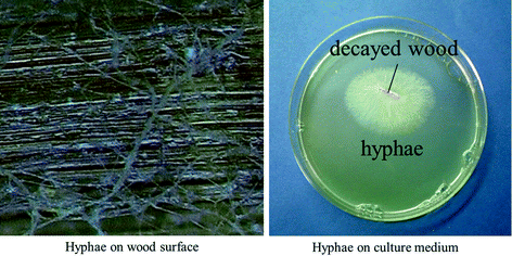

  

  Hyphae of wood-decaying fungi

  Fig. 14.48

  

  Cell wall structure, sound (left) and heavily decayed (right). Note photographs by Yuji Imamura

  Fig. 14.49

  

  Wood decay in incipient stage (left) and progressed stage (right) featured by hyphae

  Fig. 14.50

  

  Wood decay in final stages

Wood cells consist of natural polymers (polysaccharides) such as cellulose and hemicellulose. They are edible for fungi, that is, wood can be decomposed by the digestive activity of fungi such as basidiomycetes, and as a result, the density and strength decrease. Airborne spores attached to wood surfaces cause germination and division by water supplies under moderate climate conditions. The growth of hyphae will decompose the wood with enzymes, and the cell wall will be lost. The development of a fungal attack occurs when the wood is exposed to adequate temperature (0–50 °C), air (oxygen, say 20 % of wood volume), moisture (30–150 % moisture content), etc. However, the control of temperature or the removal of air is actually impossible, because the optimum conditions for these factors are almost the same as for humans. The controllable factor left behind is the moisture content of wood. So long as the moisture content of wood is kept under FSP (fiber saturation point of about 28 %), wood will not deteriorate by fungal attack, because under these conditions, no free water exists in the cellular structure, with which the fungi can grow. On the other hand, a lack of fungal attack generates in wood on extremely high moisture content (higher than 150 % or water-saturated), because the fungi cannot be exposed to a sufficient amount of air under this condition. Therefore, it follows that in order to control fungal attack in wood and wooden buildings, it is essential to control the moisture in wood. In actual wooden buildings, the water that moistens the wooden structural members is water by rain that enters through the roof or wall, water from the soil under the floor, water leaked from facilities, and dew condensed in the structures. These waters are generated in hidden or sealed areas in the buildings and are often not detectable by ordinary inspection methods in its early stage. Therefore, nondestructive detection of moisture associated with fungal attack is an essential technology.

• 2. Insect attack

Like fungi, insects attack wood as well as living trees. Well-known insects that attack wooden products are termites and beetles. They invade dried wooden members of the building and make holes by chewing and biting. As a result, the strength of wood sharply decreases.

Termites are the most significant wood-attacking insects, with more than 2200 species. About 50 species of them attack wooden buildings, with distribution mainly from tropical areas up to warm zones including North America, Oceanian, and Asian countries where wooden houses are popular. There are two types of termites: subterranean termites living mainly in the ground or moist wood and dry wood termites living in dried wood (Fig. 14.51). Termites are so-called social insects, meaning they may form colonies of 10,000 up to million worker and soldier termites. The subterranean termites live in a nest in the ground and they form a network of galleries through which they move and seek wood as bait. Once they reach a wooden building, they crawl up the structure and start attacking. Termites are adverse to light or airflow, so they crawl up in dark, hidden, or enclosed structures and materials. Usually, termites attack without notice (Figs. 14.52, 14.53 and 14.54) and it is difficult to detect the attack by visual inspection, especially at its early stage. Dry wood termites start their attack by swarming. Nymphs, after pairing, invade the wood and form a new colony. Their attack is often seen in doors, window frames, and furniture; however, they also inhabit structural members of wood, and it is difficult to discover their attack. Termites are small insects whose length is about several millimeters; however, their colonies are hugely populated and they attack wooden constructions secretly and severely. Termites attack by repeatedly chewing and bite off small fractions of wood. They attack other materials such as plastic, paper, bamboo, and concrete.

Fig. 14.51

Example of subterranean termite

Fig. 14.52

Termite galleries developed on wood under floor level

Fig. 14.53

Wood attacked by termites

Fig. 14.54

Termite attacks developing in wooden wall

Other types of dry wood-attacking insects include deathwatch beetles and powder post beetles. Adults of these insects invade wood and yield eggs. Larvae from the eggs attack the wood by chewing and biting. Like termites, it is difficult to detect the attack of beetles. It is important to have nondestructive inspection tools to detect and control the attack by termites and beetles in wood and wooden buildings.

4.2 Electrical Properties of Wood

The most important electrical properties of wood are electrical conductivity, the dielectric constant, and the loss tangent, respectively. Electric conductivity is the measure of electric current that flows in a material, when the material is placed under a given voltage gradient. The dielectric constant is the measure of the polarization or the electric potential energy induced and stored in non-conducting material, when it is placed under an alternative electric field. The loss tangent is the ratio of energy lost in the repetition of polarization. These parameters are specific for every material; however, in the case of wood, they depend on density, moisture content and anatomical features and anisotropy of the properties. There have been multiple developments for wood drying and adhesion using electrical properties. Among these, the measuring apparatus of moisture content using electrostatic capacitance is a well-known application.

4.2.1 Electric Conductivity

In a conductive material such as metal, electric current flows by the movement of free electrons. On the other hand, in non-conductive materials such as wood, the activity of the ions associated with the polar band in the cell wall and the ions derived from non-organic components in non-crystal area plays an important role. This is related to the mechanism of polarization discussed afterward.

Electric conductivity λ is given by the following formula:

$$\log \lambda = B - {C \mathord{\left/ {\vphantom {C \varepsilon }} \right. \kern-0pt} \varepsilon },$$

(14.27)

where B is a constant related to Faraday’s constant, C a constant related to energy of ionization, and ε dielectric constant, respectively.

The electric conductivity of wood is influenced by moisture content, temperature, density, and anatomical features. The most important factor is moisture content (Fig. 14.55) [36]. Electric resistance expressed as inverse of conductivity decreases linearly with moisture content from oven dry up to several percent and decreases exponentially until FSP and decreases slightly over FSP.

Fig. 14.55

Relationships between moisture content and λ and ρ for 10 European species. Note modified from the literature by Lin and by FPS [36]

Specific resistance decreases with increases in temperature, and this tendency is noticeable in lower moisture content. The influence of temperature can be attributed to the ionization in the cell. The influence of the wood species and density is not significant. Electric resistance is subjected by the cell alignment. Specific resistance in the direction normal to fiber direction is larger by 2.3–4.5 than the one in fiber direction for softwood, and by 2.5–8.0 for hardwood. The resistance in the tangential direction is slightly larger than that in the radial one. The chemical components cellulose and lignin in the wood cell wall are the origin of the electric resistance; however, the effect of the water-soluble electrolyte is larger for the moisture content over FSP. When the wood contains preservatives or fire retardant that contains metallic components and electrolytes, the resistance is larger. The properties of the resistance to alternative current (impedance) under several thousand Hz are the same for direct current, and the influence of polarization is much larger over the frequency.

4.2.2 Dielectric Constant

Dielectric constant as the measure of feasibility of polarization of a material is normally expressed as the relative value of the material’s dielectric constant to the value for vacuum state. Experimentally, it is the amount of electric quantity accumulated in a unit volume of wood by polarization, when the wood is placed under voltage gradient between a pair of electrodes. Dielectric constant for air takes 1, for water 81, for oven-dried wood 2–4, and 6.7 for dried cellulose.

The dielectric constant of wood is influenced largely by moisture content and density (Fig. 14.56) [37] and increases in accordance with moisture content. The increase becomes larger in the range of 15 up to 20 %, and it reaches about 10 at FSP of about 30 %. This increase depends on the density. For lower density (specific gravity) wood, the constant is 3 up to 5 at FSP, whereas it is about 8 for wood of specific gravity about 0.5.

Fig. 14.56

Relationships between moisture content and dielectric constant at 1 MHz for various wood densities. Note modified from the literature by Uemura and FFPRI, Japan [37]

In the moisture content over FSP, it increases largely due to the free water in the wood cell, and this is more apparent for high-density wood. The high-density wood contains more substances that take part of polarization in comparison, so that the dielectric constant becomes larger. The dielectric constant becomes larger for higher temperature. However, the increase is several percent for the temperature increase of 10 °C and is negligible for normal room temperature. The dielectric properties show anisotropy and are influenced by anatomical features of wood, especially for higher frequency. The dielectric constant decreases as the frequency increases; however, this change is strongly influenced by moisture content (Fig. 14.57) [38]. As is previously explained, it increases as moisture content for the same frequency.

Fig. 14.57

Dependence of dielectric constant on frequency and moisture content. Note for spruce, in tangential direction at 20 °C, modified from the literature by Trapp et al. [38]

4.2.3 Loss Tangent, $\tan \delta$

An ideal dielectric material releases all the accumulated energy when the electric field is eliminated by the movement of electric quantity through the connected outer circuit. However, actual dielectric materials lose energy partly in the form of heat. Power factor is the ratio of lost energy to the accumulated. Experimentally, it is related to the deviation of the electric current to the voltage gradient expressed by deviation angle (phase angle) φ, when a wood is sandwiched by a pair of electrodes and placed under an alternative electric field. The phase angle φ is the delay of current to the voltage gradient when wood is modeled electrically as a parallel circuit consisting of a resistance and a capacitance and placed under an alternative voltage gradient. The value of $\cos \varphi$ is called dielectric power factor and it varies between 0 and 1.

The angle δ as complementary angle of the angle φ is called loss angle, and $\tan \delta$ is called loss tangent. When the value of δ is much smaller than φ, loss tangent $\tan \delta$ can be approximated as $\cos \varphi$. Principally, $\tan \delta$ is given by the following formula:

$$\tan \delta = 1/2\;\pi fCR = 1.8 \times 10^{12} /\varepsilon \rho f$$

(14.28)

where f denotes frequency, C capacitance, R resistance, and ρ density, respectively.

Loss tangent is influenced by frequency, moisture content, density, and fiber orientation. It increases in accordance with moisture content but becomes much larger for higher density of wood (Fig. 14.58) [38].

Fig. 14.58

Relationships between frequency and loss tangent tan δ for various moisture contents. Note see Fig. 14.57

Loss tangent change is a complicated manner in relation to frequency and to moisture content (Fig. 14.59) [39]. It takes a maximum in the frequency range between 10⁷ and 10⁸ Hz for the wood of moisture content under 3 %. The maximum value increases in accordance with moisture content over 6.5 %; however, loss tangent takes higher values for lower frequency in accordance with moisture content. In higher frequencies, the contribution of the orientation polarization in non-crystalline area of cellulose, hemicellulose, and lignin should be important. For lower frequencies, on the other hand, the interface polarization of conductive ions should be important. Loss tangent increases as the temperature increases; however, the influence of temperature is small between 10 °C and 30 °C.

Fig. 14.59

Relationships between moisture content and loss tangent tan δ at 5 MHz. Note modified from the literature [39]

4.3 NDT of Wood Using Dielectric Properties of Wood

The most well-known apparatus and technique is the moisture meter. The dependency of electric resistance and capacitance on moisture content is applied to portable moisture meters. The moisture meter using capacitance can be applied to measure the moisture content of a relatively wide range and they evaluate the average moisture content for the area from wood surface down to a deeper area. However, the capacitance depends not only on the moisture content, but also on the density of wood, so that density adjustment is required in the measuring.

Another example is the pulse radar apparatus using microwave of the frequency range 1 to several GHz for the inspection of wood. Its aim is to detect inner holes, defects, or deterioration by catching the wave that reflected at the electromagnetic boundaries in wood. However, the difference in dielectric properties between wood and air is relatively small, so that the reflection signal is not always significant. In addition, it is difficult to obtain a higher resolution due to the frequency range and system configuration.

A radar apparatus to detect the activity of wood-attacking termites using microwave has been developed. Bodies of termites crawling in wood have high water content, creating electromagnetic boundaries in a dry wood. By observing the fluctuation of the standing wave, the activity of the termites can be evaluated.

The situation of practical NDT inspections of wooden buildings is different from the one in production lines of factories or in laboratories. In practical situations, more attention must be paid to the performance of the apparatus; for example, it should be nondestructive and non-touching, has real-time-processing affording results in 2D or 3D images, has enough measuring capacity, possesses higher resolution, and is reliable, portable, robust, and economic. Many of the apparatus previously developed use the so-called active method; that is, some physical energy such as vibration, heat, X-ray, or electromagnetic waves is given to the wood or wooden construction to be tested, then the reaction of the energy is detected in a transmitting or in a reflecting system, and the properties and state of the object are evaluated from the change in the signals. It is important that the practical apparatus should be of a reflection system, because the pair of emitter and receiver of the transmitting system cannot be applied to most of the practical situations.

In this chapter, NDT technologies for wood and wooden constructions using electromagnetic wave are introduced. In this technology, the frequency of the apparatus plays an important role. Microwave whose frequency is lower than 30 GHz transmits relatively effectively and can be applied to larger objects. It has an economical advantage; however, the resolution of imaging is relatively low for wood inspection. On the other hand, teraherz wave (0.3–3 THz) can afford extremely high resolution; however, due to the high attenuation of the wave in the material, the analysis is limited to the subsurface area, and in general, the measurement is expensive to conduct. Millimeter wave (30–300 GHz) (MMW) whose wavelength is about 10–1 mm can afford an appropriate resolution for imaging of wood, because it transmits into the wood to some extent.

4.4 Reaction of Wood to Electromagnetic Wave

4.4.1 Transmission of Millimeter Wave Through Wood

Figure 14.60 shows the setup for the millimeter wave transmitter and receiver system. A Gunn diode was used to generate the millimeter wave at an average output power of 10 mW at 100 GHz. The output signal from the diode was modulated by a PIN diode. A millimeter wave polarized linearly in vertical direction and radiated from a horn antenna is transformed into a parallel beam using a Teflon plano-convex lens. The beam was irradiated on the wood, and the transmitted wave is focused onto a sensor with another plano-convex lens. The sensor receives the electric field component parallel to the vertical direction. The received wave signal is processed in a lock-in amplifier, and the magnitude of the electric field is obtained as a voltage.

Fig. 14.60

Experimental setup of transmitting system

• 1. Transmission of MMW through wood board

Figure 14.61 shows the relationship between the fiber deviation angle θ and the magnitude of the transmitted MMW for flat-sawn boards of oven-dried cypress wood. The vertical axis denotes the ratio of transmission T (the ratio of the detected amplitude with and without wood |E_detect|/|E_in|. The transmission ratio is about 0.7 for a board of 2 mm in thickness and it decreases as the thickness increases. The transmission ratio changes periodically with the fiber deviation angle. For boards of 3–5 mm in thickness, the ratio takes the maximum for the fiber deviation angles of 90 and 270° and the minimum of 0 and 180°. For thicker boards, the number of the angle to give maximum and minimum values becomes larger. For a board of 20 mm in thickness, the minimum ratio is almost 0. There is no difference in these tendencies between flat-sawn and quarter-sawn boards.

Fig. 14.61

Dependence of millimeter wave transmission on fiber direction

• 2. Curve fitting based on theory of the transmission

The dependency of transmission ratio (attenuation) on the fiber direction can be attributed to the anisotropy of dielectric properties of wood. The mechanism of the anisotropy should be discussed in relation to the chemical components or anatomical features of wood. The main component of the cell wall is polycrystalline cellulose oriented regularly in fiber direction (–C₆H₁₂O₄–)_n. The polarization moment takes a maximum when the direction of electric field becomes parallel to the fiber direction (the orientation of cellulose polycrystalline) that is when θ=0 and 180°. As a result, the incidence of MMW attenuates and the transmitting ratio decreases. The cyclic change of transmission ratio to the fiber orientation can be attributed to the birefringent behavior of wood, and wood behaves as a retardation plate to MMW. This behavior is influenced by wavelength, wood thickness, and the anisotropy of phase shift of transmitting wave. No dependence of fiber direction on the transmitting ratio was found for the wood-based materials, such as plywood, particle board, MDF, and hardboard whose fiber orientation is random.

When wood is irradiated by MMW, attenuation and phase shift of the transmitting wave occur in addition to the reflection on the front and back surface. The reflection is featured by reflection coefficient t. On the other hand, the attenuation is featured by attenuation coefficient α, and the phase shift is featured by phase shift coefficient β. The attenuation and the phase shift are anisotropic, and coefficients α and β are separated into α_x and β_x in fiber direction and α_y and β_y in the direction normal to fiber direction, respectively. As a result, the electric field generated by the transmitting MMW changes in accordance with the deviation angle of the fiber direction to the electric field.

The transmitting ratio is expressed as follows:

$$T = t_{AW} t_{WA} \exp \left( { - \frac{1}{2}\alpha_{x} d} \right)\left| {\cos^{2} \theta + \exp \left\{ { - \frac{1}{2}\left( {\alpha_{y} - \alpha_{x} } \right)d} \right\}\exp \left\{ { - j\left( {\beta_{y} - \beta_{x} } \right)d} \right\}\sin^{2} \theta } \right|$$

(14.29)

where t_AW and t_WA denote the reflection coefficient at front or back surface and d thickness of the wood, respectively.

This formula consists of three members and they are about reflection (t_AW × t_WA), about attenuation in the material (exp(−1/2α_xd)), and about phase shift in absolute symbol, respectively. The member phase shift is related to the fiber deviation angle and wood thickness.

Furthermore, the formula takes the forms when θ = 0°

$$1 {\text{n}}\;T = - \frac{1}{2}\alpha_{x} d + 1 {\text{n}}\;t_{AW} t_{WA}$$

(14.30)

and when θ = 90°

$$1 {\text{n}}\;T = - \frac{1}{2}\alpha_{y} d + 1 {\text{n}}\;t_{AW} t_{WA}$$

(14.31)

The logarithm of the transmission ratio ln T is linear to the thickness d. The gradient corresponds to the attenuation coefficient at the given fiber deviation angle and the intercept the coefficient of reflection (Fig. 14.62) [40]. From the linear regression formula, the value of attenuation coefficient in the fiber direction is obtained as α_x = 0.13 (/mm), the one in the normal direction as α_y = 0.08 (/mm), and the reflection coefficient of 0.85.

Fig. 14.62

Relationships between specimen thickness and transmitting ratio. Note modified from the literature by Tanaka [40]

• 3. The influence of moisture content

Figure 14.63 shows the dependence of the transmitting ratio on the fiber deviation angle of the test board at different moisture contents. The transmitting ratio decreases as the moisture content increases, and the dependency on the fiber direction becomes less significant. The moisture in wood absorbs MMW. The anisotropic factor expressed as the ratio of transmission ratios, along and normal to fiber direction, increases in accordance with in moisture content and takes a maximum value at about 150 %, and again decrease for higher moisture content as shown in Fig. 14.64. One possible reason is as follows: In moisture range under 150 %, water molecules are adsorbed to the cell wall and they are allocated as if the profile of the cell wall structure was enhanced, and as a result, the anisotropy of the transmitting ratio is enhanced. On the other hand, in the case of higher moisture content, the cell cavities are filled with water molecules and their allocation in fiber direction is diminished, and the factor of anisotropy becomes smaller. The coefficient of the attenuation of MMW in wood becomes larger as the density for both directions, along and normal to fiber direction, respectively. However, the attenuation can be different in wood species of the same density, and this suggests that anatomical features influence attenuation. More detailed discussion on MMW in the transmission in wood can be found in literatures by Tanaka et al. [41, 42].

Fig. 14.63

Dependence of transmission on moisture content of Japanese cypress

Fig. 14.64

Dependence of anisotropy in transmittance on moisture content

4.4.2 Reflection of MMW from Wood

The behavior of millimeter wave in a reflection detection system was also investigated using a monostatic system of millimeter wave of 94 or 100 GHz (Figs. 14.65 and 14.66) [43, 44]. This apparatus is monostatic using a circulator. A Gunn diode was used to generate the millimeter wave at an average output power of 10 mW at 100 GHz. The output signal from the diode was modulated by a PIN diode, polarized and irradiated to the surface of wood through a circulator and waveguide probe whose cross section is square of 3 by 2 mm and 50 mm long. The reflected component is received by the same waveguide and sent through circulator to a Schottky diode for square law detection. The detected signal is sent to a lock-in amplifier, and the magnitude of the reflection is measured. This measurement is conducted by scanning of the wood specimen attached to a XY-table to get the 2D distribution of reflected amplitude. The distance between the aperture of the waveguide and the wood can be adjusted by 1 mm, and the direction of fiber can be set parallel or normal to polarization direction.

Fig. 14.65

Experimental setup for reflection imaging using 100 GHz  millimeter wave [43, 44]

Fig. 14.66

System configurations

Imaging of surface and subsurface of finished wood was conducted. Figure 14.67 shows an example of image taken by scanning of wood block using reflection imaging by a monostatic system. In the scanning of wood surface finished with Japanese lacquer (Fig. 14.67a), the pattern of a wood grain orientation under the lacquer layer was clearly recognized (Fig. 14.67b). To clarify the penetration depth of millimeter wave into wood specimen, another test was conducted to detect the layer of aluminum foil inserted between a pair of cut wood blocks (Fig. 14.67c). In the reflection image, a characteristic stripe pattern is recognized near the left side of the image (Fig. 14.67d). This result was caused by the change in the amplitude of the wave that is radiated to the wood, penetrated into the wood and reflected at the foil. The stripe pattern can be attributed to the interference of the penetrating wave with the reflected one. The existence of the inserted foil can be recognized at a depth of about 15–18 mm at the deepest case for the tested 5 wood species.

Fig. 14.67

Example of scanning using reflection system [43, 44]

Figure 14.67 right shows an example of a reflection image of a small wood specimen taken from a post in a Buddhist temple (left). It was attacked by beetles and contains several holes. Some visible defects are also seen on the surface. The surface of the block was scanned by a millimeter wave apparatus. On the reflection of millimeter wave image, several characteristic shaded areas (dot line circles) are seen and they suggest the existence of inner defects.

The distribution of inner defects was also evaluated by a microfocus X-ray CT apparatus (SMX-160CT-SV3-S, SHIMADZU Corp.). This was compared with the MMW image. Characteristic changes can be seen in the X-ray image (left) corresponding to the shaded areas (dot line circles) suggesting inner defects in the MMW image. However, some other unique shaded areas can be also seen in the X-ray image. They can be attributed to the holes and galleries made by beetles at deeper positions, and they could not be detected by the millimeter wave imaging.

Another feasibility of reflection system is the detection of wood-attacking insects in the wood. Figure 14.68 [45] shows a time-domain signal of millimeter wave detected by reflection imaging system when a millimeter wave is irradiated on the surface of a wood specimen behind which a different number of living worker termites are put in a bottle. Millimeter wave is reflected at the electromagnetic boundary between wood and the insect, and this causes characteristic fluctuation of the amplitude. The frequency of the fluctuation depends on the number of termites inhabited. These results show that millimeter wave technology can be a useful nondestructive monitoring tool of activity of biological agents.

Fig. 14.68

Detection of wood-attacking insects inhabiting wood

4.5 Wall Scanner for Diagnoses of Wooden Houses

4.5.1 Technical Background

Nondestructive inspection is one of the essential technologies for the structural health assessment of timber structures. Its aim is to analyze the structural property and other attributes, such as durability. The authors have recently developed a small radar apparatus for the nondestructive evaluation of wooden walls typically found in Japanese wooden family houses [46]. Two objectives were set in the development of this tool: to visualize the inner structure of the wall, giving us important information related to the evaluation of anti-earthquake resistance of the house, and to see the biodegradation or moisture distribution of inner wood related to the durability of the house (Figure 14.69) [46].

Fig. 14.69

Target walls for NDT using FMCW technique

4.5.2 Devices [46]

The first developed experimental apparatus is a small scanner equipped with a horn antenna for sending and receiving of the electromagnetic wave attached to a vertical XY-stage of 400 by 400 mm of working area, a signal processor for generation and detection of electromagnetic wave, a controller for the XY-stage, and a small personal computer for the control of the measuring system (Figs. 14.70 and 14.71).

Fig. 14.70

Scanning devices with antenna

Fig. 14.71

Experimental setup of FMCW radar system to get time-domain signal

The apparatus works according to FMCW (frequency-modulated continuous wave) radar technology. The electromagnetic wave has a sweep range of 10–20 GHz emitted from the antenna and is irradiated to the wooden wall to be investigated. A part of the wave is reflected at the wall surface, but the rest of it transmits the wall. The transmitting components reflect partly at electromagnetic boundaries in the wall such as interfaces between wooden parts and the metal parts, between inner cavities and substantial parts such as wood or metal, and between moist areas and dried areas. The reflected wave components are received by the antenna and detected by the signal processor.

In the signal processor, a beat signal is composed by synthesizing the source signal and the detected one. By analyzing the beat signal, the intensity and the location of the reflection are obtained as the amplitude and the delay of peaks in the time-domain signal. By scanning of the antenna in the vertical plane using XY-stage and taking the data with an interval, the distribution of the intensity of the reflected signal in any vertical plane in the wall is obtained. At the same time, the change in the intensity of the reflected signal along the wall thickness at any point in the vertical plane is also obtained. By scanning, the time-domain signal can be displayed as 2D or 3D images, and it is possible to recognize the shape, the size, and the allocation of the members in the wall.

4.5.3 Performance of Wall Scanner for Structure Analysis [46]

Figure 14.72 shows an example of time-domain signal detected for a simple model wall structure consisting of two pieces of plywood of 12 mm in thickness and set at a distance of 95 mm. The time-domain signal can be obtained by the inverse FFT of the beat signal from the detector.

Fig. 14.72

Time-domain signal showing feasibility of detection of objects hidden in a model wall [46]

The horizontal axis denotes time, but actually it denotes the distance in the direction of wall thickness from the antenna. Two peaks are detected and they are the reflection of the two boards. The position of each peak corresponds to the location of the board, and the peak value changes in accordance with the dielectric constants of the board. The low peak found between the two peaks can be attributed to the multireflection of the wave in the system and it seems like a ghost.

Figure 14.73 shows similar results except when a thin metal plate is attached to the backside of the board. The electromagnetic wave reflects at a boundary of dielectric properties. Larger reflection occurs at the boundary of the larger difference in dielectric properties. At the surface of metal, it reflects larger, and as a result, the peak in the detected signal becomes higher.

Fig. 14.73

Time-domain signal from model wooden wall

The performance of the apparatus was evaluated using a model wooden wall consisting of posts, beams, and a stud, and covered with a piece of plywood or a plaster board whose thickness is 12 mm (Fig. 14.74). The wooden members are assembled by metal plate connectors, bolts, and coarse thread screws. The posts and beams are made of laminated lumber whose cross-sectional dimension is 120 mm in square, and the stud made of solid wood is 45 mm in thickness. The wooden members are all made of dried softwood. The structure is a simplified model of the wall structure frequently found in modern Japanese wooden family houses constructed according to the posts and beams method.

Fig. 14.74

Two-dimensional image of scanning of sample wooden wall

This wall was scanned, and the results are shown in a contour map of the amplitude of the detected signals in a section at a distance from the antenna. The red area corresponds to the corner metal plate assembled in the wall, and the shape, the size, and the allocation of the plate can clearly be recognized. The wooden construction members such as studs, posts, and beams were also recognized, although the amplitude of the reflected signal was smaller than the one from the metallic parts. The volt of 12 mm in diameter in the post was also detected, so long as it is allocated at a depth less than 40 mm from the surface.

These results show that the apparatus is able to provide us important structural information hidden in the wall with a covering board. We have applied this method also to the Japanese traditional clay wall, and it was confirmed that the network made of bamboo strips (lath) set in the clay wall for the reinforcement was roughly recognized.

Figure 14.75 shows a distribution of the intensity of the reflected wave in a vertical section in the wall. The shape of the corner plate can be recognized easily. This distribution can be obtained at any layer of different distances from the antenna. As a result, the wall structure can be evaluated three-dimensionally. This is similar to the one obtained by computer tomogram (CT) technique using an X-ray apparatus. But the largest difference between them is that CT works in a transmitting system, whereas the wall scanner works in a reflection system. As already discussed, it is absolutely necessary to have a device of reflection system for practical NDT for buildings and other types of structures.

Fig. 14.75

Three-dimensional image of wall structure estimated by multiplying 2D distribution of reflection intensity

4.5.4 Performance of Wall Scanner for Biodegradation

When the wooden members in the wall are deteriorated biologically, for example, when they are attacked by termites or decayed by fungal attack, wood substance disappears and is accompanied by a decrease in strength, and this causes a change in the detected signal. More importantly, the biodegradation of wood is closely associated with the moisture in the wall. This moisture would be normally derived by water leaking through the covering of the wall or the condensation at the thermal boundaries in the wall structure. On the other hand, the electromagnetic properties of wood vary by the moisture content of wood, so that it can be expected that by detecting the area of higher moisture content by the change in the reflecting electromagnetic wave, the possibility of biodegradation in the wooden members of the wall can be evaluated.

To confirm this idea, decayed wood plate of different moisture contents were prepared. They were sandwiched between a pair of polypropylene films and attached to the backside of a wall covering board. The board was scanned from the front side by the developed apparatus (Fig. 14.76). At the position of decayed wood plate of higher moisture content, significantly higher amplitudes of the reflected signal from the board were detected, although the peak amplitudes were lower than the ones from a metal plate attached to the back side of the board. The layered 2D images of the scanning show the distribution of higher peak amplitude corresponding to the moist and decayed wood plate and can be clearly recognized (Fig. 14.77). Under this condition, the area of moisture content is higher than the FSP and can be significantly detected, at which fungal activity in wood becomes higher.

Fig. 14.76

Detection of moist wood hidden behind surface board

Fig. 14.77

Visualization of dry wood (left) and moist-decayed wood (right) hidden behind surface board

Detection of decayed wood behind a sound covering board was also attempted. Artificial decayed wood of thin Japanese larch and Japanese fir boards exposed to fungal attack for 2–12 weeks (weight loss 2–50 %) was attached to the backside of a wall covering board, and this was scanned from the front side. It was confirmed that the decayed specimen in wet state was clearly recognized. However, the dried one was not always detected successfully. The result was that the electromagnetic wave was reflected at the boundary between the plaster board and the moist wood.

4.5.5 Development of a Portable Wall Scanner “Wood Wall Viewer”

Based on basic studies, a small radar apparatus was developed (Fig. 14.78) [46]. The apparatus consists of a small device and a personal computer. The principle of the detection is the same as the previous experimental one, but without the XY-stage and controller for scanning. The device is an all-in one type involving an antenna, electric circuits for sweep generation and detection of the electromagnetic wave, a data processing unit, and a battery. It is convenient to use for detection at one spot on a wall by attaching the device by hand, but it can be scrolled on the wall manually. The data are sent to a PC through USB interface and postprocessed by the developed control software. The detected signal is displayed on PC in the form of real-time time-domain signal in the manner of FIFO processing. By adjusting the analysis condition and by eliminating the signal caught for base or standard conditions, the target objects can be detected more precisely.

Fig. 14.78

“Wood wall viewer” using FMCW radar system

Figure 14.79 shows some results of detection for a model wall consisting of two boards, face and back, set apart by 90 mm. The wall was scanned from the face side. A metal plate attached to the backside of the face board or to the front side of the back board is detected clearly. Studs of a smaller dimension located in the wall were also detected. A wood specimen of different moisture contents attached to the back side of the face board was also recognized. The intensity of the reflection increased in accordance with the moisture contents. On the other hand, some ghost peaks caused by the multiple reflections in the wall were detected.

Fig. 14.79

Results of scanning using “Wood wall viewer”

4.6 Automatic Recognition of NDT Data Using Pattern Recognition

4.6.1 Introduction

The data obtained by NDT are in the form of signal, and 2D or 3D images and they often contain not only the information related to the target objects but also the influence of other factors or noise. For the proper interpretation of the data, the experience and knowledge of skilled inspectors are required. In this section, a technology of pattern recognition applied to an automatic interpretation of image data and to the recognition of defects in wood is introduced.

4.6.2 RCE Network

The technology of pattern recognition is an example of information process that recognizes an object, and actually, it is a flow (algorithm) of information process often expressed in the form of computer program. To recognize the object is to decide the category to which it belongs. For this purpose, a series of data measured from the object called “pattern” expressed in the form of vector is inputted into the program for pattern recognition and the program gives us the category as output. The dimension of the vector is the number of the data measured from the object. For example, in order to judge a man, whether he is healthy or unhealthy, we can prepare a vector of parameters such as blood pressure, weight, height, and age and input it into the pattern recognition program, and then, the program gives us a answer “healthy” or “unhealthy” as output.

The pattern is a vector of nth dimension, and the vector space of nth dimension is called pattern space. Patterns derived from the objects which belong to a category occupy a certain subspace in the pattern space. The patterns of another category occupy another area in the pattern space. In the technology of pattern recognition, the boundary between subspaces is decided as first. This is the process to construct the mechanism of pattern recognition. Secondly, after the mechanism is established, we can put unknown pattern into the program and get the answer. The answer is the category to which the unknown pattern belongs.

The boundary between subspaces in a nth pattern super-space is expressed as super-plane of (n−1)th dimension. To construct the mechanism of pattern recognition in other words, divide the pattern super-space by super-planes of (n−1)th dimension. In many cases, the subspace occupation is complex and it is not easy to set the boundaries. To solve this issue, many kinds of algorithms for multilayered neural networks are used. For the construction of the mechanism, a training method using training patterns is used. By this method, an optimum recognition algorithm is constructed automatically, as if the computer receives the final algorithm by training by itself. RCE network is a kind of neural network, and its feature is to get the mechanism by less training. In this section, an application of RCE network to wood inspection is introduced.

RCE network is basically a three-layered network consisting of input, middle, and output layers. In the training of the RCE network, the mechanism of pattern recognition is established by the following process: (1) A training pattern whose category is already known is placed in the pattern space, and then, a small area of the category is acquired around an input training pattern. (2) By the repeating this process, a body of subspace gathered by the small areas of the category is formed in the pattern space. However, if the area of a category around a training pattern interferes with the area of other categories, then the size of each area is adjusted so that the interference is eliminated. (3) The process is repeated until all the training patterns can be located in the subspace of the right categories. The training process of the RCE network is relatively simple and it requires less training.

Figure 14.80 [47] shows an example of application of the RCE network to the automatic diagnosis of blue-stained wood. By adopting pattern vectors of multiple elements derived from the analysis of color components of pixels, the areas of blue-stained and sound were recognized successfully. By taking the training patterns, mechanisms of diagnosis can be established flexibly according to the local variation and features of the woods. Once the mechanism is established by training, an automatic diagnosis is proceeded quickly by non-touching method and nondestructively.

Fig. 14.80

Pattern recognition of 2D image using RCE network. Note modified from the literature by Sawada [47]

References

Jackson JD (1962) Classical electrodynamics. Wiley, New York
Smythe WB (1989) Static and dynamic electricity, 3rd edn. CRC Press, Boca Raton
Bell JR, Leonards GA, Dolch WA (1963) Determination of moisture content of hardened concrete by its dielectric properties. In: Proceedings of the American society for testing and material, vol 63
Irie H, Yoshida Y, Sakurada Y, Ito T (2008) Non-destructive-testing methods for concrete structures. In: NTT Tech Rev 6(5). https://www.ntt-review.jp/archive/ntttechnical.php?contents=ntr200805le3.pdf&mode=show_pdf
Light ESPAR 2, AIREC Engineering Corporation. http://www.airec.co.jp/products/html/000056.html
Taniguchi T, Kobayashi T (2003) An omnidirectional and low-VSWR antenna for the FCC-approved UWB frequency band. In: Proceedings of the 2003 IEEE AP-S international symposium, Columbus, USA, June 2003, pp 460–463
Kobayashi T, Takahashi N, Yoshikawa M, Tsunoda K, Tennno N (2007) Measurement of automobile UWB radar cross sections at Ka band. In: Sabath F, Mokole EL, Schenk U, Nittsch D (eds) Ultra-wideband short-pulse electromagnetics 7. Springer, New York, pp 586–592
Taniguchi T, Maeda A, Kobayashi T (2007) An omnidirectional and low-VSWR ultra wideband antenna for a frequency band of 6 to 40 GHz. In: Braun CE, Stone AP, Tyo JS (eds) Ultra-wideband, short-pulse electromagnetics 8. Springer, New York, pp 41–48
Yang T, Davis WA (2004) Planar half-disk antenna structures for ultra-wideband communications. In: Proceedings of the 2004 IEEE AP-S international symposium, Monterey, USA, June 2004, pp 2508–2511
Hirota A, Iwasaki H (2005) Planar trapezoid dipole antenna with ultra wideband characteristics. In: Proceedings of the 2005 IEEE AP-S international symposium, Washington D.C., USA, July 2005, pp 540–543
H. Sato, K. Sawaya, N. Arai, Y. Wagatsuma, and K. Mizuno “Broadband FDTD analysis of Fermi antenna with narrow width substrate,” in Proceedings of the 2003 IEEE AP-S International Symposium, Columbus, USA, June 2003, pp. 261–264
Kim IK, Kidera N, Pinel S, Papapolymerou J, Laskar J, Yook J-G, Tentzeris MM (2006) Linear tapered cavity-backed slot antenna for millimeter-wave LTCC modules. IEEE Antennas Wirel Propag Lett 5:175–178
Uehara K, Miyashita K, Natsume K, Hatakeyama K, Mizuno K (1992) Lens-coupled imaging arrays for the millimeter-and submillimete-wave regions. IEEE Trans Microw Theory Tech 40(5):806–811
Mizuno K (2001) Millimeter wave imaging technologies (invited). In: Proceeding of the 2001 Asia-Pacific microwave conference, Taipei, December 2001, pp 394–398
Lee RQ, Simons RN (1997) Advances in microstrip and printed antennas, In: Lee HF, Chen W (ed) chapter 9, Wiley, New York
Sugawara S, Maita Y, Adachi K, Mori K, Mizuno K (1997) A mm-wave tapered slot antenna with improved radiation pattern. In: IEEE MTT-S international microwave symposium digest, Denver, USA, pp 959–962
Sugawara S, Maita Y, Adachi K, Mori K, Mizuno K (1998) Characteristics of a mm-wave tapered slot antenna with corrugated edges. In: IEEE MMT-S international microwave symposium digest, Baltimore, USA, pp 533–536
Takagi Y, Sato H, Wagatsuma Y, Sawaya K, Mizuno K (2004) Study of high gain and broadband antipodal fermi antenna with corrugation. International Symposium Antennas and Propagation, vol 1, Sendai, Japan, pp 69–72
Wang S, Chen XD, Parini CG (2007) Analysis of ultra wideband antipodal vivaldi antenna design. In: Proceedings of the 2007 Loughborough antennas and propagation conference, Loughborough, UK, April 2007, pp 129–132
Gu K, Wang G, Li J (2004) Migration based SAR imaging for ground penetrating radar systems. IEE Proc Radar Sonar and Navig 155:317–325
CST STUDIO SUITE 2006B, Computer simulation technology GmbH http://www.cst.com
Kaneko S, Oka S, Matsumiya N (2012) Detection of cracks in concrete structures from digital camera images. NTT Technical Review, vol 10, No. 2, 2012. https://www.ntt-review.jp/archive/ntttechnical.php?contents=ntr201202fa3.html
Oka S, Mochizuki S, Togo H, Kukutsu N (2009) Inspection of concrete structures using millimeter-wave imaging technology. NTT Tech Rev 7(3). https://www.ntt-review.jp/archive/ntttechnical.php?contents=ntr200903sf4.html
Sheen DM, McMakin DL, Hall TE (2001) Three-dimensional millimeter-wave imaging for concealed weapon detection. IEEE Trans Microw Theory Tech 49(9):1581–1592
Ravan M, Amineh RK, Nikolova NK (2010) Near-field microwave holographic imaging: target localization and resolution study. In: 2010 URSI international symposium on electromagnetic theory, Aug 2010, pp 396–399
Kak AC, Slaney M (2001) Principles of computerized tomographic imaging. Society of Industrial and Applied Mathematics, Philadelphia
Mochizuki S, Oka S, Togo H, Kukutsu N (2010) High-phase-resolution 77-GHz-band radar module for near-field millimeter-wave imaging. In: 2010 IEEE MTT-S international microwave symposium Digest, May 2010, pp 636–639
Guidelines for concrete crack inspection, maintenance and reinforcement (2013) Japan Concrete Institute (in Japanese), http://www.jci-net.or.jp/j/publish/book/guide_0080.html
Yamaguchi T, Nakamura S, Hashimoto S (2008) An efficient crack detection method using percolation-based image processing. In: Proceeding of the industrial electronics and applications, ICIEA, in Singapore, pp 1875–1880
Oka S, Mochizuki S, Togo H, Kukutsu N (2009) A neural network algorithm for detecting invisible concrete surface cracks in near-field millimeter-wave images. In: Proceeding of the IEEE international conference on systems, man, and cybernetics, neural networks and their applications II, in Texas, pp 3901–3905
Ogami M (1987) Hand Book of Image Processing. Tokyo University Publication (in Japanese)
Fujita Y, Mitani Y, Hamamoto Y (2006) A method for crack detection on a concrete structure. In: Proceeding of IEEE 18th international conference on pattern recognition, Hong Kong, 20–24 Aug 2006
Serre T, Wolf L, Poggio T (2005) Object recognition with features inspired by visual cortex. In: Proceeding of IEEE computer society conference on computer vision and pattern recognition, San Diego, 20–25 Jun 2005
Yamaguchi T, Nakamura S, Hashimoto S (2008) An efficient crack detection method using percolation-based image processing. In: Proceeding of industrial electronics and applications, ICIEA, Singapore, pp 1875–1880
Markwardt LJ, Wilson TRC (1935) Strength and related properties of woods grown in the United States. In: Technical Bulletin 479, USDA Forest Products Laboratory 99 p
Lin T (1967) Review of the electrical properties of wood and cellulose. For Prod J 17(5):54–60
Uemura T (1960) Dielectrical properties of woods as the indicator of the moisture. Bull For For Prod Res Inst 119:95–167
Trapp W, Pungs L (1956) Einfluss von Temperatur und Feucht auf das Dielectrische Verhalten von Naturholz im grossen Frequenzbereich. Holzforschung 10(5):144–150
Standard of wood processing using high frequency electricity (1960) Technical report of The Institute of Electrical Engineers of Japan, 38
Tanaka S, Fujiwara Y, Fujii Y, Okumura S, Togo H, Kukutsu N, Nagatsuma T (2011) Effect of grain direction on transmittance of 100-GHz millimeter wave for hinoki (Chamaecyparis Obtusa). J Wood Sci 57(3):189–194
Tanaka S, Fujiwara Y, Fujii Y, Okumura S, Togo H, Kukutsu N, Mochizuki S (2013) Dielectric anisotropy of oven- and air-dried wood evaluated using a free space millimeter wave. Journal of Wood Science, Springer, doi:10.1007/s10086-013-1341-7, published April 2013
Tanaka S, Fujiwara Y, Fujii Y, Okumura S, Togo H, Kukutsu N, Mochizuki S (2013) Effect of annual rings on transmission of 100 GHz millimeter waves through wood. Journal of Wood Science, Springer. doi: 10.1007/s10086-013-1342-6, published April 2013
Fujii Y, Fujiwara Y, Tanaka S, Okumura S, Togo H, Mochizuki S, Kukutsu N (2010) Feasibility of millimeter wave imaging as tool for nondestructive inspection of wood and wooden structures. Proceedings of 35th international conference on infrared, millimeter and terahertz waves, Roma, September 2010. doi:10.1109/ICIMW.2010.5612351
Fujiwara Y, Fujii Y, Tanaka S, Okumura S, Togo H, Mochizuki S, Kojima T, Kukutsu N (2012) Feasibility of imaging technology using micro- and millimeter wave for nondestructive inspection of wooden buildings. Proceedings of advanced electromagnetics symposium, AES 2012, proceedings, Paris, April 2012, pp 672–674
Fujii Y, Fujiwara Y, Yanase Y, Okumura S, Narahara K, Ngatsuma T, Yoshimura T, Imamura Y (2007) Nondestructive detection of termites using a millimeter-wave imaging technique. For Prod J 57(10):75–79
Fujii Y, Fujiwara Y, Yanase Y, Mori T, Yoshimura T, Nakajima M, Tsusumi H, Mori M, Kurisaki H (2013) Development of radar apparatus for scanning of wooden-wall to evaluate inner structure and bio-degradation non-destructively. Adv Mater Res 778:289–294
Sawada Y, Matsumoto A, Fujii Y (2015) Pattern recognition of blue stain discoloration appeared on radiata pine boards. Mokuzai Gakkaishi 61(4):274–279
Author information
Authors and Affiliations
Corresponding author
Editor information
Editors and Affiliations
Rights and permissions
Copyright information
© 2015 Springer-Verlag London (outside the USA)
About this chapter
Cite this chapter
Togo, H., Oka, S., Fujii, Y., Fujiwara, Y. (2015). Nondestructive Visualization Using Electromagnetic Waves for Real and Practical Sensing Technology for Robotics. In: Liu, Z., Ukida, H., Ramuhalli, P., Niel, K. (eds) Integrated Imaging and Vision Techniques for Industrial Inspection. Advances in Computer Vision and Pattern Recognition. Springer, London. https://doi.org/10.1007/978-1-4471-6741-9_14
Download citation
DOI: https://doi.org/10.1007/978-1-4471-6741-9_14
Publisher Name: Springer, London
Print ISBN: 978-1-4471-6740-2
Online ISBN: 978-1-4471-6741-9
eBook Packages: Computer ScienceComputer Science (R0)