Modeling Combustion with Detailed Kinetic Mechanisms

Blurock, Edward; Battin-Leclerc, Frédérique

doi:10.1007/978-1-4471-5307-8_2

Edward Blurock⁴ &
Frédérique Battin-Leclerc⁵

Part of the book series: Green Energy and Technology ((GREEN))

3265 Accesses
4 Citations

Abstract

Detailed chemical kinetic combustion models of real fuels (e.g., gasoline, diesel, and jet fuels) provide important chemical insight into the chemical phenomena behind the combustion process. The challenge is to find computationally feasible models that help explain the complex behavior observed during the combustion of complex mixtures of hydrocarbon species which make up real fuels. Detailed kinetic mechanisms, made up of a set of reactions and species, describing the chemical reactions between fuel, oxidizer, and intermediate species have proven to be useful in providing the link between the macroscopic phenomena and the microscopic behavior. The purpose of this chapter is to outline the structure, role and diversity of detailed mechanisms in combustion modeling. An important emphasis of this chapter is to describe the approximations and assumptions used. Within the set of chemical modeling methods in general, the interaction between detailed mechanism modeling and more complex chemical models, such as quantum chemical models, or much simpler models, such as skeletal, semi-detailed, and even global reaction mechanisms, is outlined.

Access provided by Autonomous University of Puebla. Download chapter PDF

Structural analysis of combustion mechanisms

Article 28 September 2014

Unsteady Combustion Processes Controlled by Detailed Chemical Kinetics

Reduced Kinetic Models for Methane Flame Simulations

Article 01 March 2019

Keywords

These keywords were added by machine and not by the authors. This process is experimental and the keywords may be updated as the learning algorithm improves.

1 Introduction

A model is an interpretation and an approximation of physical reality. A model is not only a representation of physical reality, but also a construction helping to understand the governing principles behind the physical reality and to make predictions about physical behavior. In a sense, there is only one physical reality, but there can be a multitude of models representing it. A particular model represents a particular aspect the modeler focuses on. A model can serve multiple purposes. Two significant purposes of a model are understanding and prediction. Of course, these are not mutually exclusive. A “thorough” (the word is in quotes because the model is an approximation of reality) understanding implies that predictions are possible. The level of understanding described by the model is inherently coupled with the complexity and detail of the model. A detailed kinetic mechanism is one such model with its own set of assumptions which are detailed in this chapter for the field of combustion.

In early civilization, the power of the combustion phenomenon was ruled by gods with many mythological names such as Zhu Rong (Chinese), Kagu Tschuchi (Japanese), Hephaestus (Greek), and Vulcan (Roman). In the seventeenth century, Johann Joachim Becher explained the thermodynamics of fire with his phlogiston theory. In the eighteenth century, the role of oxygen and other molecules in combustion became apparent in Lavoisier’s and Priestley’s experiments and the chemical nature of the combustion process and matter itself began to be explored. The study of thermodynamics of combustion was spurred by the industrial revolution with the fundamental theories of Carnot (Carnot 1824) and Gauss (Dunnington et al. 2003; Gauss 1823) which are still in use. At the time of Faraday’s treatise and lecture, “The Chemical History of the Candle” (Faraday 1861), the interactions of the fundamental thermodynamics and chemical aspects of the flame were emerging. With Semenov’s theory of chain mechanisms and thermal explosions (Semenov 1935, 1958) the modern science of detailed combustion reactions began.

Studies of detailed kinetic mechanisms not only have the scientific importance of understanding nature around us, specifically the combustion process, but now they have environmental importance in trying to minimize man’s contribution to climate change, industrial economic importance in making the combustion process in flames, engines, and turbines in transportation and energy more efficient, and socio-political importance in helping to minimize the use of fuels. The goal of a comprehensive detailed mechanism is to extensively describe combustion phenomenon at a chemical level. Of course, without a first principle means of identifying all relevant species and reactions, we can only approximate this goal. Within a collisional dynamic framework, in order to explain the macroscopic nature of the combustion process, we would not only have to identify all the colliding species but also the frequency and energetics of all the collisions under the extensive range of temperatures, pressures, and reacting compositions found, for example, in engines.

To describe ignition properties, whether in zero-dimensional homogeneous combustion or including also diffusion effects in multidimensional combustion, a model has to describe a whole range of temperature regimes. The models first have to reproduce macroscopic phenomena such as laminar flame velocities, ignition delay times, extinction strain rates, or turbulent or oscillatory behavior. They also have to explain the relative concentrations of the fuel and oxidizer and a range of intermediate species including pollutants in premixed and non-premixed regimes. In addition, the models have to consider the wide range of combustion time scales found from simple one-dimensional to turbulent three-dimensional flames.

With the lack of a universal model of combustion, model design decisions have to be made. A major source of diversity in combustion models, even for the same fuel, stems from the modeler choosing the “important” properties and parameters needed to describe the chosen physical phenomenon as shown in the comparison of methane combustion models made by Rolland and Simmie (2004). Every model has its advantages and disadvantages. An important aspect of computer modeling is computational cost. Modeling detail in one aspect often comes at the price of neglecting another aspect. For example, with current computational resources, it is impossible to formulate an exact model of jet fuel, gasoline, or diesel fuel with their immense number, diversity, and size of fuel elements (see Fig. 2.1).

Not only does the modeler have to simplify a complex fuel composition with surrogates (see Sect. 2.6.5) but also to reduce the size of the map of operating conditions to be covered. Very few detailed models are valid for wide ranges of temperatures, pressures, or equivalence ratios. The key to the simplification of models, for example in the writing of reduced models or skeletal mechanisms (see Sect. 2.6.3 or for more details Chap. 17), is to limit the range of operating conditions to be considered. In zero-dimensional models, such as in the cases of homogeneous ignition in a rapid compression machine or oxidation in a perfectly stirred reactor, very detailed mechanisms (e.g. Sarathy et al. 2011; Westbrook et al. 2009) can be used. However, for computational fluid dynamic calculations, where there is extensive detail in the three-dimensional flow of the reacting species, only very simplified models, such as global or possibly skeletal mechanisms can be used. There is always a modeling trade-off between chemical detail and physical or flow detail in a model.

Detailed combustion modeling plays an important role in elucidating reactive behavior under different conditions and in identifying the pathways leading to pollutant emissions in order to propose reduction methods. For example, Fig. 2.2 shows that at higher equivalence ratios, the amount of soot increases. But at lower equivalence ratios, as the temperature increases, the amount of NOx emissions increase. At low temperature and equivalence ratio, both soot and NOx emissions are low. It is under these conditions that the combustion in homogenous charge compression engine (HCCI) or in diesel low temperature combustion (LTC, an alternative approach to achieve HCCI-like combustion obtained by coupling closely autoignition to fuel injection (Dec 2009)) engines function (see Fig. 2.2). It is why it is expected to have lower emissions. Kinetic studies using detailed mechanisms play an integral part of the development HCCI or LTC diesel engines.

2 Chemical Combustion Models

There are a multitude of techniques to model a chemical process (e.g. Williams 1994; Tomlin et al. 1997; Griffiths and Barnard 1995; Warnatz et al. 2006). The focus of this chapter is one particular type of modeling, namely with detailed combustion mechanisms. But before presenting them some general features of chemical mechanisms are discussed.

2.1 Generalities About Chemical Mechanisms

At the simplest level, a chemical mechanism can be seen as just a list of reacting species and a list of their reactions. However, this and other chapters in this book will try to elaborate the considerable structure and detailed chemical and kinetic knowledge required behind these lists. To begin with, two sets of information are provided within the mechanism formulation. There is the thermodynamic information mainly represented by the thermochemical quantities associated with each species, and the kinetic information associated with the set of reactions detailing how the set of species react with each other.

Each reaction in a combustion mechanism is a description of how a set of reactant species are transformed into a set of product species. Ultimately, this description is transformed to numerical combustion models, which solve the mass and the energy conservation equations, according to the type of reactor with special software libraries dedicated to that, such as CHEMKIN (Kee et al. 1993).

An essential component of the numeric form describing chemistry is the chemical source term, i.e., the rate of change of concentration of the reacting species, which is extensively described in textbooks (Laidler 1987; Griffiths and Barnard 1995; Warnatz et al. 2006). For example, reaction i in the set of m _reactions in a mechanism including n _species species can be generally written:

$$ \sum\limits_{k = 1}^{{n_{\text{species}} }} {\nu}_{ki}^{\text{reactants}} {\text{X}}_{k} = \sum\limits_{k = 1}^{{n_{\text{species}} }} {\nu}_{ki}^{\text{products}} {\text{X}}_{k} $$

(2.1)

where ν _ki is the stochiometric coefficient related species X _k in reaction i. The rate of progress, $ q_{i} $ of reaction i can then be expressed:

$$ q_{i} = k_{i}^{\text{reverse}} \prod\limits_{k = 1}^{{n_{\text{species}} }} {\left[ {X_{k} } \right]}^{{{\nu}}_{ki}^{\text{products}} } - k_{i}^{\text{forward}} \prod\limits_{k = 1}^{{n_{\text{species}} }} {\left[ {X_{k} } \right]}^{{{\nu}}_{ki}^{\text{reactants}} } $$

(2.2)

where $ \left[ {X_{k} } \right] $ is the molar concentration of species X _k and $ k_{i}^{\text{foward}} $ and $ k_{i}^{\text{reverse}} $ are the forward and reverse rate constants of reaction i. This, in turn, is used to compute the rate of production (ω _k) of species X _k:

$$ \omega_{k} = \prod\limits_{i = 1}^{{n_{\text{reactions}} }} {({\nu}_{ki}^{\text{reverse}} - {\nu}_{ki}^{\text{forward}} )q_{i} } $$

(2.3)

This is commonly known, especially in reactive flows associated with CFD (computational fluid dynamics) equations, as the chemical source term.

An important point is that even when writing down the initial chemical form, the species within the reactions are only labels, i.e., bookkeeping devices keeping track of their concentrations. The actual structural information is only implied by how the species react and the thermodynamic information associated with each species. As shown in the chemical source term, the numeric rate constants combined with the species concentrations form the heart of reactive chemistry.

Rate constants, k, are usually expressed using the classical Arrhenius (Arrhenius 1889) form of the rate expression, shown here with a temperature exponent:

$$ k = AT^{n} e^{{E_{a} l\;RT}} $$

(2.4)

where A is the pre-exponential factor, n is the temperature coefficient, E _a is the activation energy, and R is the gas constant in J·K⁻¹. More details about rate constant format are given in Chap. 19.

Associated with each species is their temperature-dependent thermochemical data, specifically enthalpy, entropy, and heat capacities (see more details in Chap. 20). In combustion, this thermodynamic information is usually represented as two seven term “NASA polynomials,” first formulated by Zeleznik and Gordon (1962):

$$\begin{aligned}\frac{{C_{p} }}{R} & = a_{1} + a_{2} T + a_{3} T^{2} +a_{4} T^{3} + a_{5} T^{4} \\ \frac{{H^{o} }}{RT} & = a_{1}+ a_{2} \frac{T}{2} + a_{3} \frac{{T^{2} }}{3} + a_{4} \frac{{T^{3}}}{4} + a_{5} \frac{{T^{4} }}{5} + \frac{{a_{6} }}{T} \\ \frac{{S^{o} }}{R} & = a_{1} {\kern 1pt} {\text{In}}T +a_{2} T + a_{3} \frac{{T^{2} }}{2} + a_{4} \frac{{T^{3} }}{3} +a_{5} \frac{{T^{4} }}{4} + \textit{a}_{7} \end{aligned}$$

(2.5)

The temperature, T, dependent heat capacity, C _p, standard Enthalpy, H ^o, and standard Entropy, S ^o are represented with seven species dependent constants, a_i. Note that associated with each species are also their transport properties to be used for the evaluation of gas-phase multicomponent viscosities, thermal conductivities, diffusion coefficients, and thermal diffusion coefficients (see for instance, Wang and Frenklach (1994)).

2.2 Detailed Chemical Mechanisms

A detailed chemical mechanism is usually considered to be composed of a particular type of reaction, namely, an elementary reaction (also called elementary step). An elementary reaction is a transition from a (set of) reactant molecular structure(s) to a (set of) product molecular structures. The transformation from the reactant molecular structures to the product molecular structures can be thought of the movement of the individual atoms making the reactants through intermediate structures until they reach the product molecular structures.

When the modeler writes down the reactants and products of an elementary reaction, he thinks about the complex molecular changes such as valence changes and the making and breaking of bonds that occur during the reactions (see Sect. 2.4). The rate constant associated with each elementary reaction is derived from the molecular structure and is not dependent on conditions under which it is measured, except temperature and in some cases pressure (for more detail, see Chap. 21). Many rate constants relevant to combustion can be obtained from databases (e.g., Baulch et al. 1992; Tsang and Hampson 1986), evaluating experimental measurements and theoretical calculations; for more detail, see Part V about rate constant determinations. For more than 2 decades, data evaluations, as those shown in Fig. 2.3, have been performed to assess the available kinetic data and then, based on these assessments, recommended rate constants with their uncertainties have been proposed.

The reaction taken as an example for Fig. 2.3 also illustrates an important feature of combustion mechanisms: the involved molecular structures are not always stable molecules, but in many cases free radicals (or even atoms), e.g., uncharged species with an unpaired electron. Reactions involving free radicals can be divided in four types:

Initiation: those creating radicals from fuel,
Termination: those consuming radicals,
Propagation: those transforming a radical into another one,
Branching : those creating new radicals from a radical or an unstable product (degenerate branching steps).

Several types of elementary reactions have pressure-dependent rate constants, e.g., unimolecular fuel decomposition (see Sect. 2.4.2). In this case, many combustion models use the formalism proposed by Troe (1974), an extension of the Lindemann-Hinshelwood theory (Laidler 1987), to express the pressure-dependent rate constant, k, as a function of the rate constant at very low pressure k ₀, the rate constant at infinite pressure, k _∞, and [M] the total concentration of all the present species (third body). These expression for k with four reaction dependent constants, a, T*, T**, and T***, can also be found in recommendation compilations such as (Baulch et al. 1992). Note that at very low pressure, k can be approximated by k ₀[M], and then increases until k _∞ which is obtained at very high pressure. In between the evolution of k versus [M] followed a “fall off” curve which can be approximated by Eq. (2.6). The low-pressure rate constant, k₀, depends also on the nature of the third body gas. Third-body efficiencies are also specified in detailed models and can vary up to a factor of 18 between the least efficient gas, He, and the most efficient one, H₂O (Husson et al. 2013). While third-body efficiencies can have a significant influence, such as explaining a priori surprising acceleration of autoignition by addition of water (Anderlohr et al. 2010), important uncertainties exist in their values.

$$\begin{aligned}\frac{k}{{k_{\infty } }} & = \frac{y}{1 + y}F(y)\;\left({{\text{with}}\; \, y = \frac{{k_{0} [M]}}{{k_{\infty } }}} \right)\\ \log \,F(y) & \,\cong \, \frac{1}{{1 + \left[ {\frac{\log (y)}{n}}\right]^{{^{2} }} }}\log \,F_{\text{cent}} \;({\text{with}}\;n = -0.75 - 1.27\;\lg \;F_{\text{cent}} ) \\ F_{{{\text{cent}} .}} & = (1 - a)\,\exp \left( { - \frac{T}{{T^{\ast \ast \ast} }}} \right) + a\,\exp \left( { - \frac{T}{{T^{\ast} }} } \right) + \exp \left( {- \frac{{T^{\ast \ast}}}{T}} \right) \end{aligned} $$

(2.6)

The purpose of detailed mechanisms is not only to a posteriori reproduce given experimental results, but also to encompass a priori predictions of behaviors for which experimental investigation is difficult, even impossible, or too costly. Detailed mechanisms are also an invaluable tool that can give further chemical understanding of the chemical kinetic processes and species involved. Note that detailed mechanisms are used also for chemical modeling in other fields than combustion, such as atmospheric chemistry (Bloss et al. 2005) or astrochemistry (Venot et al. 2012).

Of increasing importance is computational chemistry based on electronic structure theory, quantum chemistry (Lewars 2011), and semi-empirical models for calculating the needed thermodynamic and kinetic constants. With the increased computational power of modern computers, more complex molecular systems can be calculated. These calculations can not only be used to substantiate experimental evidence, but often they can be used where experiments are very difficult or not even possible. In these models, an explicit three-dimensional structure of the combustion species is specified and its energy structure is derived.

Essentially, a single computational chemistry calculation starts with a three-dimensional configuration of atoms and is based on the resolution of the Schrödinger equation using different levels of assumptions (Harding et al. 2007; Pilling 2009). One of the fundamental assumptions is the Born–Oppenheimer approximation which separates the solution involving the nuclei and the electrons, i.e., the nuclei are assumed to be stationary. Given this atomic configuration, the orbital (and total) energy of the molecule is calculated. The Hartree–Fock approximation using a “Slater Determinant” representation of the electronic orbital wavefunctions (for further details see, for example, (Levine 2000)), enables the numerical calculation of this molecular energy. These orbital wavefunctions are represented in terms of basis sets (Hill 2013). The level, accuracy, and complexity of the computation largely depend on these basis sets. More details are given in Chap. 20.

Since the temperature-dependent thermodynamic constants used in combustion are dependent on the total and internal energy of a molecule, computational chemistry calculations are an ideal way to make systematic thermodynamic studies of classes of species. For example, studies have been made for n-alkanes (Vansteenkiste et al. 2003) or a wide rage oxygenated molecules or radicals (Sumathi and Green 2002; Sebbar et al. 2004, 2005; Da Silva and Bozzelli 2006; Simmie et al. 2008; Yu et al. 2006).

A single computation of an atomic configuration in three-dimensional space gives a single molecular energy. If “all” configurations of a set of atoms are calculated a potential energy surface (Lewars 2011) of these configurations can be calculated (see for example, Fig. 2.4). This potential energy surface can be used in molecular dynamics calculations to calculate rate constants (see Chap. 21). Uncertainties in these rate constant calculations are discussed by Goldsmith et al. (2013). Figure 2.4 displays the paths connecting reactants and products for two competing elementary steps in an energy diagram. The needed information in this complex energy surface is reduced to the “lowest energy” path between the reactant configuration and the product configuration. Each path has to overcome a thermodynamic barrier to form an activated complex called transition state or transition structure (Eyring 1935; Truhlar et al. 1996; Harding et al. 2007). As with individual species, each activated complex has its own thermochemical properties which can be calculated using computational methods (see Chap. 20). It can be shown that the energy to form this transition state from the reactants is the activation energy used in the Arrhenius form of the rate constant (Gilbert and Smith 1990).

2.3 Low and High Temperature Detailed Chemical Combustion Mechanisms

Advanced low temperature combustion concepts that rely on compression ignition have placed new technological demands on the modeling of the low temperature reactions of O₂ with fuel (oxidation) in general and particularly on fuel effects in autoignition. Furthermore, the increased use of alternative and nontraditional fuels presents new challenges for combustion modeling and demands accurate rate coefficients and branching fractions for a wider range of reactants. Fuels, especially for transport industry, have long-chain hydrocarbon components.

This includes even the long-chain methyl esters of biodiesel. The study of the ignition of hydrocarbons is intimately related to several aspects of engine performance such as timing, efficiency, and emissions. Numerous books and reviews such as (Griffiths and Barnard 1995; Westbrook 2000; Battin-Leclerc et al. 2011; Zádor et al. 2011) have described the chemistry involved during ignition.

Figure 2.5 shows a simplified scheme of the main primary reactions, which are now usually included in models of the oxidation of an alkane (RH) according to the understanding previously gained (Pollard 1977; Kirsch and Quinn 1985; Walker and Morley 1997; Miller et al. 2005). Alkyl radicals (R·) are produced from the reactant (RH) by hydrogen atom abstractions (H-abstractions), first during a short initiation period, by O₂, and then primarily by ·OH radicals. At low temperatures, i.e., below 900 K, R· radicals add to O₂ to yield peroxy (ROO·) radicals.

Some consecutive steps then lead to the formation of hydroperoxides, which are degenerate branching agents, explaining the high reactivity of alkanes at low temperature. The ROO· radicals first isomerize to give hydroperoxyalkyl (·QOOH) radicals. This isomerization, which occurs via an internal H-abstraction going through a cyclic transition state, has a very large influence on the low temperature oxidation chemistry (Kirsch and Quinn 1985). According to the size of the cyclic ring involved in the transition state, the formation of alkenes and ·HO₂ radicals can compete with isomerization, mainly at low temperature, by direct elimination from ROO· (Zádor et al. 2011)

·QOOH radicals can thereafter add on O₂ and yield ·OOQOOH radicals. These react further by a second internal isomerization producing ·U(OOH)₂ radicals. The rapid unimolecular decomposition of ·U(OOH)₂ radicals leads to three radicals and is a branching step occurring at low temperatures. This global step occurs through the formation of alkylhydroperoxides including a carbonyl group, mainly ketohydroperoxides, which in turn can easily decompose giving two radicals. The proposed ketohydroperoxides have only been recently experimentally detected (Battin-Leclerc et al. 2010) under conditions observed close to autoignition. In this scheme, a ·OH radical reacting by H-abstraction with the initial alkane leads to the formation of three free radicals, two ·OH, and a XO· radicals, in a chain reaction. This auto-acceleration process strongly promotes the oxidation of alkanes below 700 K.

When the temperature increases, the equilibrium R· + O₂ = ROO· begins to shift back to the reactants and the formation of ROO· radicals is less favored compared to the strongly inhibiting formation of ·HO₂ radical and the conjugated alkene. This reaction is equivalent to a termination step since ·HO₂ radicals react mostly by a disproportionation reaction (2 ·HO₂ = H₂O₂ + O₂). Unimolecular decompositions of ·QOOH radicals also compete with O₂ addition; ·QOOH radicals can decompose into cyclic ethers, aldehydes or ketones and ·OH radicals, or by β-scission into ·HO₂ radicals and conjugated alkenes or smaller species. Because of the decrease in the production of hydroperoxides, the reactivity decreases in the 700–800 K temperature range.

This temperature region exhibits a counterintuitive behavior and is called the region of negative temperature coefficient (NTC). As shown in Fig. 2.3 in the NTC region, the ignition delay times show the opposite of “normal” behavior, namely that the ignition delay time increases with increasing temperature. This phenomenon had been experimentally observed for many years but could not be satisfactorily explained until kinetic modeling was used to simulate the process. Extension of this type of kinetic analysis eventually led to a thorough description of the kinetics of engine knock, octane number, and HCCI ignition. Examples of experimental observations of NTC zones, as well as modeling using detailed kinetic mechanisms, are presented in Fig. 2.6. Note that in Fig. 2.6 models can fairly well reproduce the position of the NTC area and its variation with pressure, which shifts toward higher temperature when pressure increases. This shift is due to the influence of pressure on the equilibrium of the addition reactions of molecular oxygen to the alkyl and hydroperoxyalkyl radicals (Curran et al. 1998).

NTC is also an explanation for another specificity of the oxidation of alkane chemistry; the possible occurrence of cool flame phenomenon at temperatures several hundred degrees below the minimum autoignition temperature. During a cool flame, or multiple cool flames, the temperature and the pressure increase strongly over a limited temperature range (typically up to 500 K), but the reaction stops before combustion is complete due to the decrease in reactivity in the NTC zone. The review paper of Townend (1937) shows when this phenomenon was beginning to be accepted and systematically explored.

At higher temperatures, the decomposition of H₂O₂ (H₂O₂ (+M) = 2 ·OH (+M)) is a new branching step leading to an increase of the reactivity. This reaction becomes very fast above 900 K. Above about 900 K, the small alkyl radicals (R′·) obtained by the decomposition of the initial alkyl radicals can in turn decompose to give alkenes and ·H atoms. The reaction of ·H atoms with oxygen leads to ·OH radicals and ·O· atoms, which in turn regenerates ·OH radicals by H-abstraction from the fuel. This reaction is the main branching step ensuring the full development of the ignition and the complete combustion.

The chemical behavior just discussed has lead to two different types of detailed mechanisms:

A low and intermediate temperature mechanism which considers the addition to oxygen of alkyl radicals. This mechanism is of maximum complexity, and consequently usually of very large size, but it is absolutely needed to predict the chemistry occurring in or below the NTC zone.
A high temperature mechanism which neglects the addition to oxygen of alkyl radicals. This mechanism is much less complex and of much limited size, but it can only be used to predict the chemistry occurring above the NTC zone, i.e., above 1000 K. The high temperature mechanism is well adapted for flame modeling for which diffusion effects have to be considered.

3 Species and Molecular Representation

A molecule (taken in a wide sense including both stable molecules and free-radicals) is a complex object with a multitude of model representations. Each model focuses on what physical reality should be modeled. For example, within physics, the forces and particles within the nucleus of the molecule are important to describe radioactive phenomenon. Within a computational chemistry model, the nucleus is essentially a point charge and the model is concerned with the “structure” and energy of the electron shells around the nucleus (Hehre 2003; Cramer 2004). In this model, each molecular configuration (positions of the nuclei within the molecule) has an energy and this information is used to deduce spectroscopic, thermodynamic, and reactive properties. But even within computational chemistry there is a wide range of possible representations (Davidson and Feller 1986), each with differing computational complexity and accuracy. In semi-empirical molecular models, quantum mechanical models are simplified using parameterization and the focus is on the valence electrons which are the key to chemical reactivity (Stewart 2007). In simpler organic chemistry models, such as Lewis structure (Lewis 1916; Gillespie and Robinson 2007), molecules are represented as atoms with bonds to other atoms and valence electronic properties (e.g., Balaban 1995).

3.1 Molecular Representations in Detailed Mechanisms

Within combustion, a multitude of modeling levels and representations of molecules are used. As outlined previously, the species representation within detailed mechanisms is actually just a label in a reaction and each label has some thermodynamic information associated with it. The actual complex structure of the individual species of the mechanism is encapsulated in the information in this representation. The thermochemical data is related to the molecular structure and bonding of the molecule with its functional groups and is a condensation of the complex molecular energies within a molecule. Aside from direct experimental data, another source of thermochemical data can indeed be computational chemistry computations. The rate constants are essentially a condensation of the change of molecular configuration over a complex potential energy surface as discussed in Sect. 2.2.2.

Determining which molecules and reactions to use in the detailed combustion mechanism can be said to be the result of analyzing and studying the reactivity of each species. Although kinetic and thermodynamic details emerge with experimental and computational analysis, initial guesses can be made by analyzing the “Lewis structure” of the species. This will be discussed in the next section.

3.2 Lewis Structures and Detailed Combustion Modeling

It is common in organic chemistry to use Lewis structures (Lewis 1916; Gillespie and Robinson 2007) to describe the fundamental properties of molecules and how they react. The Lewis structure description, basically, describes the molecule as one writes it down on a piece of paper; a set of atoms connected with a set of (multiple) bonds and possibly the existence of lone pairs and unpaired electrons (radicals) on the atoms. It is synonymous with the 2D graphical form (Balaban 1985), where the graphical nodes are the atoms with associated atomic information, such as atomic number, charge, and if it has a radical or lone pairs. The bonding information between these nodes tells which atoms are bonded together and how they are bonded, i.e., single, double, or triple bond and possibly if the bond has aromatic or resonant character. When the modeler writes molecules or reactions on a piece of paper, some of the implied three-dimensional character of the molecule is included. Figure 2.7 illustrates the cyclic structure of the six-membered ring and the tetrahedral nature of the 5 sp³-bonded carbon and oxygen atoms (for more complete explanation of bonding at this level consult any organic chemistry textbook, such as (Clayden et al. 2012)) that is needed to set up the intramolecular hydrogen abstraction during an isomerization of a peroxy radical obtained during the oxidation of n-decane.

The Lewis structure model is particularly useful in visualizing the radical behavior of species in combustion reactions. For example, Fig. 2.8 shows how “electron pushing” (see for example Levy (2008)) describes how an alkyl radical can decompose to form a radical and a double bond. The key to this analysis is that a bond is made up of two shared electrons. In the first (virtual) step, the shared electrons go to their respective carbon atoms. In the second step, the newly formed radical electron and the other radical become “shared” to form the second bond of the double bond. Using this level of analysis, a large portion of hydrocarbon combustion reactions can be explained and new reactions can be postulated. This technique is very common in organic chemistry.

3.3 Functional Groups

Lewis structures using electron pushing is a way to keep track and to analyze reactive behavior. However, the effect of different atoms, such as oxygen which plays a large role in hydrocarbon combustion, and different bonding, such as single, double, triple, resonant, and aromatic, is supplementary physical chemical information that has to be taken into account by the modeler. Every chemical environment, meaning an atom and its bonding, has an effect on the neighboring atoms and bonds. For example, a radical on a carbon atom is more energetically stable on a tertiary carbon atom than on a primary carbon atom which has the consequence that a tertiary hydrogen atom is more easily extracted from the carbon atom. These different types of hydrogen and carbon atoms are shown in Fig. 2.9.

Single-bonded oxygen atoms are more electronegative than, for example, carbon atoms and thus they draw electrons toward them thus weakening directly connected bonds. The concept used extensively in organic chemistry is that of the functional group, i.e., a (small) collection of atoms and bonds forming a chemical group which have distinct properties (for more information the reader can peruse almost any organic chemistry textbook or, for example (Trahanovsky 1971; Byrd and Hildreth 2001; Struyf 2009)). Functional groups are not only used to describe properties, but also to describe classes of molecules. For example in detailed combustion modeling, particularly those describing hydrocarbon oxidations, mechanisms can include n-alkanes, branched alkanes, alkyl radicals, olefins, allyl radicals, alcohols, aldehydes, ketones, aromatics, oxy radicals, peroxy radicals, hydroperoxyradicals, cyclic compounds, and furans. Without resorting to basic physical chemistry principles or even computational chemical principles, the modeler can refer to classes of reactions involving these functional groups. Those groups which are particularly important in combustion modeling are discussed in Sect. 2.4.1, “Concept of Reaction Classes.”

3.4 Molecular Representation and Reactivity

In order to understand chemical reactivity, how a molecule is represented and what information this representation contains is central. This applies for both modeling and for experiments. For example, for modelers trying to simulate experimental results, the representation of the molecule can be as simple as a number for the concentration of the species at a given time and/or place in the reactive system. Behind this representation lie other models and representations of the molecule. A spectroscopist measuring the concentration of a species identifies the species by its spectral features, often functional groups, which can involve the electronic or vibrational structure of the molecule; see for example Pretsch et al. (2009). The molecule is then represented by its spectrum. Of course, to describe the physical origin of the spectrum, even more detailed model representations, from statistical mechanical to quantum mechanical models are needed. Even within these models, there lie many levels of modeling and representations.

For the numerical simulation of combustion processes lay also many levels of models and representations. As discussed in Sect. 2.2.1, a common representation of a molecule in combustion is a species label with associated thermodynamics and reactivity. But once again, behind this representation can be a multitude of more detailed representations. For example, when a modeler creates a mechanistic step, the Lewis bonding representation could be used. What is important in this representation is keeping track of the valence electrons which could be involved in a bond, where each atom contributes an electron per bond— a paired electron in a lone pair occupying a valence orbital or a radical, a single electron without a pair in an orbital. For more complex structures, the modeler can draw the bonding on a piece of paper in the 2D graphical form. Here, the three-dimensional structure of the molecule is only implied.

For example, the intramolecular abstraction of a hydrogen atom by a peroxyl group presented in Fig. 2.7 can be written in several ways, each showing a bit more information about the reactive step. The reaction could first be written as follows:

$$ {\text{C}}_{ 10} {\text{H}}_{ 2 1} {\text{OO}} \cdot \to \cdot {\text{C}}_{ 10} {\text{H}}_{ 20} {\text{OOH}} $$

(2.7)

This emphasizes the hydrogen atom being extracted from an internal carbon atom creating a radical and the making of a hydroperoxy (OOH) bond. There is no indication whether the abstraction is from the primary or secondary carbon atom, how branched are the carbon atoms and other thermodynamic influences, such as the ring strain, needed to execute this transformation. This information however could be indirectly given in the associated rate constant. If this reaction is found in a reduced scheme (see Sect. 2.5.3), then the species labels could represent a lumped species and the reaction itself represents a set of lumped reactions.

To take into account the set of possibilities undergoing this intramolecular hydrogen abstraction, more information and more reactions would have to be written. To make the distinction as to where the intramolecular abstraction is taking place, several more species labels are created and several more reactions are written. One such reaction could be written as:

$$ {\text{C}}_{10} {\text{H}}_{21} {\text{OO}}\! \cdot\!{\hbox{-}}{\text{3}}\to \cdot {\text{C}}_{ 10} {\text{H}}_{ 20} {\text{OOH}}{\hbox{-}}\text{3 }\! {\hbox{-}}\text{1} $$

(2.8)

where the ‘1’ refers to the carbon atom from which the hydrogen atom was extracted and the ‘3’ refers to the carbon atom where the peroxyl group is. That this reaction is dealing with a linear alkane would be implicit from the reaction mechanism. It should be noted that one often sees this type of name due to the name length restrictions when converting the list of reactions for the numeric solver. Longer labels could be used to give a representation reflecting the long straight chain of the reacting species. For example, the same reaction could be written:

$$\begin{aligned}& {\text{CH}}_{ 3} {\text{CH}}_{ 2} {\text{CH}}({\text{OO}}\cdot ){\text{CH}}_{ 2} {\text{CH}}_{ 2} {\text{CH}}_{ 2}{\text{CH}}_{ 2} {\text{CH}}_{ 2} {\text{CH}}_{ 2} {\text{CH}}_{ 3}\to \\ & \cdot\!\! {\text{CH}}_{ 2} {\text{CH}}_{ 2}{\text{CH(OOH)CH}}_{ 2} {\text{CH}}_{ 2} {\text{CH}}_{ 2}{\text{CH}}_{ 2} {\text{CH}}_{ 2} {\text{CH}}_{ 2} {\text{CH}}_{ 3} \end{aligned}$$

(2.9)

One important structural feature apparent in both the reactions 2.8 and 2.9 is that the hydrogen atom is abstracted from a primary carbon atom, i.e., one of the three hydrogen atoms at the terminal carbon atom in the hydrocarbon chain. The three-dimensional structure is more apparent if the same structures are drawn in 2D graphical form as in Fig. 2.10. Although the molecule is written on a flat 2D surface, the three-dimensional structure is implied through the zigzag drawing and the partial ring.

The position of the hydrogen atoms from the carbon atoms can be emphasized more by using a special notation used by organic chemists as shown in Fig. 2.7. The carbon atoms are drawn in a zigzag pattern in the plane of the paper. The dashed extended triangle denotes that the bond goes into the paper and the filled in extended triangle comes out of the paper. A simplistic bonding is implied with all bond lengths being about the same and that even the oxygen has a tetrahedral configuration. With the 2D graphical form, two important features which can affect the rate constant of this particular reaction are revealed. The bond and valence changes occurring at the atoms within the reactive species are described and the structure of transition state is implied. In the abstraction process of Fig. 2.7, a six-membered ring is formed. The rate constant should reflect further information about the abstraction being from a primary carbon atom and the ring strain due to the formation of a six-membered ring transition state.

For the current example (see Fig. 2.7), the reactive center, i.e., just those atoms involved in the reaction, consists of the carbon–hydrogen bond which is broken in the course of the reaction and the oxygen radical which abstracts the hydrogen:

$$ {\text{O}}\! \cdot + {\text{ C}}\! - \!{\text{H}} \to {\text{O}}\! - \!{\text{H }} + {\text{ C}} \cdot $$

(2.10)

However, the local molecular environment around the reactive center is what determines the first approximation to the rate constants. The local environment is the set of atoms and bonds, which are connected to the atoms carrying the reactive center. An example is a functional group. It is the job of the modeler to decide the extent of the local environment which has a significant effect on the rate constant. It should always be kept in mind that what is considered “significant” depends on the level of modeling being considered. In this particular example, a very significant feature is that the oxygen is in a peroxy functional group (as opposed to, for example, oxy radicals). An additional significant local feature is the type of carbon atom from which the hydrogen atom is abstracted, i.e., whether it is a primary, a secondary, or a tertiary carbon atom. This particular reaction has not only local “electronic” effects, but also a non-local steric effect and ring strain can affect the rate constant. In contrast to the “electronic” local features effecting the bond strength and radical stability, this is due to the structure of the transition state of the reaction. In this reaction, the transition state involves a ring structure determining which local effects should be considered is dependent on the level of modeling. This is a key assumption in determining reaction classes which will be discussed in the next section.

4 Reactions

As discussed previously, reactions in detailed mechanisms represent a transformation from one species to another. All the physical information associated with the reaction, whether it comes from experiments, simple physical chemistry arguments, or more complex calculations, is implied in the rate constants of the reaction and the thermodynamic data of the species. This gives considerable freedom in how the reaction is written.

There is no fundamental restriction as to the level of mechanistic detail a reaction class should represent. As discussed previously, a reaction in a detailed mechanism is a transformation from reactants to products. In essence, the only restriction is that the rate of this transformation can be represented in an Arrhenius form with possible pressure-dependent parameters (see Sect. 2.2.2). The following are some examples of types of reactions that can usually be considered:

Elementary reaction: these are fundamental mechanistic steps, for example through one transition state.
Formally direct reaction: these are reactive pathways that traverse more than one transition state in a single elementary step (Zádor et al. 2011).
Vertical lumped reaction: the reaction formally goes through several transition states, but only the initial reactants and the final products are given in the reaction.
Lumped species reaction: some or all of the species, reactants, and/or products, listed in the reaction are lumped (see Chap. 17).
(Semi-)global reactions: a transition between a set of reactants to a set of products not necessarily representing any mechanistic structure.

Note that, to be considered a detailed mechanism, a mechanism should not consist mostly of lumped or (semi)-global reactions. In this case, it should be called semi-detailed mechanism.

For some elementary reactions, the full potential energy surface can be complex. Indeed in reactive systems where multiple reactive possibilities occur, the potential energy surface can have several minima, for the reactants and products, and transition states for the activated species. In understanding the system, however, the important information can be condensed to a diagram such as Fig. 2.11, where multiple minima and transition states (as maxima with a given activation energy) are shown. Figure 2.11 shows the path from butyl radical to hydroperoxybutyl radical can occur in two ways. The first is given as two consecutive “simply direct” elementary reactions, for example:

$$ {\text{CH}}_{ 3} {\text{CH}}_{ 2} {\text{CH}}_{ 2} {\text{CH}}_{ 2} \cdot + {\text{O}}_{ 2} \to {\text{CH}}_{ 3} {\text{CH}}_{ 2} {\text{CH}}_{ 2} {\text{CH}}_{ 2} {\text{OO}} \cdot \to \cdot {\text{CH}}_{ 2} {\text{CH}}_{ 2} {\text{CH}}_{ 2} {\text{CH}}_{ 2} {\text{OOH}} $$

(2.11)

In addition, however, there is a “formally direct” (Zádor et al. 2011) pathway directly from the butyl radical to the hydroperoxybutyl radical, for example:

$${\text{CH}}_{ 3} {\text{CH}}_{ 2} {\text{CH}}_{ 2} {\text{CH}}_{2}\!\cdot + {\text{O}}_{ 2} \to \cdot {\text{CH}}_{ 2} {\text{CH}}_{ 2}{\text{CH}}_{ 2} {\text{CH}}_{ 2} {\text{OOH}}$$

(2.12)

Formally direct pathways are single elementary steps, but they are mechanistically “indirect,” crossing sometimes multiple transition states. Their rate constants are more difficult to calculate than for “normal” elementary reactions. They can be derived from eigenvector-eigenvalue pairs in the solution to the master equation (see Chap. 21).

For practical purposes, reactions in most detailed mechanisms are not restricted to elementary steps. For example, in the secondary mechanism of hydrocarbon oxidation automatically generated by the EXGAS mechanism automatic generation software (more details can be found in Biet et al. (2008) or in Chap. 3), some reactions are vertically lumped so as to produce as products small species (including two or less carbon atoms) in only one reaction. For example, the addition of hydroxyl radicals to an alkene is written:

$$ {\text{OH}} \!\!\cdot + {\text{C}}_{\text{n}} {\text{H}}_{{ 2 {\text{n}}}} \to {\text{HCHO}} + \!\!\cdot \text{C}_{({\rm n}\hbox{-}{1})} \text{H}_{(2n-1)} $$

(2.13)

where n is the number of carbon atoms in the linear hydrocarbon.

Reactions in detailed kinetic mechanisms can also sometimes be written using horizontal lumping, i.e., using lumped species. For example, in the n-hexadecane oxidation of Westbrook et al. (2009), the alkenyl species are lumped into one generic species, C₁₆H_31, which represents all combinations of positions of the double bond and the radical center so that for example:

$$ \begin{aligned} & {\text{OH}} \!\cdot + 1{\hbox{-}} {\text{C}}_{ 1 6} {\text{H}}_{ 3 2} \to {\text{H}}_{ 2} {\text{O}} + \cdot {\text{C}}_{ 1 6} {\text{H}}_{ 3 1} \\ & {\text{OH}} \!\cdot + 2{\hbox{-}} {\text{C}}_{ 1 6} {\text{H}}_{ 3 2} \to {\text{H}}_{ 2} {\text{O}} + \cdot {\text{C}}_{ 1 6} {\text{H}}_{ 3 1} \\ \end{aligned} $$

(2.14)

More generally, outside the strict scope of detailed mechanisms, reactions can also have “global” or “semi-global” properties. Semi-global reactions can be found within “semi-detailed” mechanisms. For example, in the mechanism of the oxidation of n-decane of Ranzi et al. (2005), the decomposition of decyl radicals (R_10•) is represented in a semi-global reaction:

$$\begin{aligned}{\text{R}}_{ 10} \cdot \to & 0.0 5 1 6 {\text{CH}}_{ 3}\! \cdot +0. 1 3 3 2 {\text{C}}_{ 2} {\text{H}}_{ 5}\! \cdot + 0. 1 4 7 5{\text{C}}_{ 3} {\text{H}}_{ 7} \cdot \\ & + 0. 1 4 7 5{\text{C}}_{ 4} {\text{H}}_{ 9} \!\cdot + 0. 20 4 {\text{R}}_{ 5}\!\cdot + 0. 2 8 7 {\text{R}}_{ 7} \!\cdot + 0.0 3 {\text{R}}_{ 10}\!\cdot + 0.0 8 8 9 {\text{C}}_{ 2} {\text{H}}_{ 4} + 0. 1 5 6 9{\text{C}}_{ 3} {\text{H}}_{ 6} \\ & + 0. 1 4 1 2 {\text{C}}_{4} {\text{H}}_{ 8} + 0. 20 7 {\text{C}}_{ 5} {\text{H}}_{ 10} + 0. 32 7 {\text{nC}}_{ 7} {\text{H}}_{ 1 4} + 0.0 7 8 8 {\text{nC}}_{ 10}{\text{H}}_{ 20}\end{aligned}$$

(2.15)

One extreme example is the global combustion reaction proposed by Westbrook and Dryer (1981) which represents a whole mechanism of a hydrocarbon fuel:

$$ {\text{Fuel}} + n_{ 1} {\text{O}}_{ 2} \to n_{ 2} {\text{CO}}_{ 2} + \, n_{ 3} {\text{H}}_{ 2} {\text{O}} $$

(2.16)

4.1 Concept of Reaction Classes

Producing detailed combustion mechanisms for the oxidation of fuels with a large number of carbon atoms in its structure (larger than three) presents several shifts in mechanism production philosophy. First and foremost, it cannot be expected that the source of the rate constants be exclusively from experiments. The individual reactions that appear in mechanisms with larger hydrocarbons, due to their variety, complexity, and size, most likely do not have (and the majority never will have) isolated experiments giving direct rate constant information. For this reason, estimates of the reaction rate constants must come from general physical chemical principles. One way of encompassing and translating these general principles into specific reactive properties is to define reaction classes.

Reaction classes are kinetic generalizations that systematically embody the analogies and physical principles the modeler has to use to make educated guesses for the rate constants for reactions where no experimental evidence exists. The key assumption when using reaction classes is that only a local set of functional features around the reactive center (see Sect. 2.3.5) are significant when determining the numeric value of the rate constant. The concept of reaction classes is not restricted to automatic generation of detailed mechanisms. Even in the generation of large mechanisms by hand, reaction classes are used to produce detailed mechanisms. One example is the n-hexadecane mechanism of Westbrook et al. (2009).

A reaction class has essentially three sets of information:

1.
A pattern or rule to recognize within the chemical reactants (can be more than one) when the reaction class should be applied,
2.
A transformation of how the specific reactants are converted to products,
3.
The rate constants associated with the transformation.

4.2 List of Reaction Classes Usually Used in Combustion Mechanisms

While reactions classes are slightly different depending on authors (see discussion by Battin-Leclerc 2008), there is some agreement for the main ones. In their mechanisms of the oxidation of n-heptane (Curran et al. 1998), isooctane (Curran et al. 2002) and C₇–C₂₀ methylalkanes (Sarathy et al. 2011), the team of Livermore has defined reactions classes, which are certainly used in literature in detail. Those recently proposed by Sarathy et al. (2011) are listed below (reactions classes in italics are part of the secondary mechanisms, see Sect. 2.5.1):

High temperature reaction classes:
1. 1.
  Unimolecular fuel decomposition
2. 2.
  H-atom abstraction from the fuel
3. 3.
  Alkyl radical decomposition
4. 4.
  Alkyl radical isomerization
5. 5.
  H-atom abstraction reactions from alkenes
6. 6.
  Addition of radical species ·O· and ·OH to alkenes
7. 7.
  Reactions of alkenyl radicals with ·HO ₂, ·CH ₃ O ₂ , and ·C ₂ H ₅ O ₂
8. 8.
  Alkenyl radical decomposition
9. 9.
  Alkene decomposition
10. 10.
  Retroene decomposition reactions
Low-temperature reaction classes:
1. 11.
  Addition of O₂ to alkyl radicals (·R + O₂ = ROO·)
2. 12.
  R· + ROO· = RO· + RO·
3. 13.
  R· + HO₂· = RO· + OH·
4. 14.
  R· + CH₃OO = RO· + CH₃O·
5. 15.
  Alkyl peroxy radical isomerization (ROO· = ·QOOH)
6. 16.
  Concerted eliminations (ROO· = alkene + ·HO₂)
7. 17.
  ROO· + HO₂· = ROOH + O₂
8. 18.
  ROO· + H₂O₂ = ROOH + HO₂
9. 19.
  ROO· + CH₃O₂· = RO· + CH₃O· + O₂
10. 20.
  ROO· + ROO· = RO· + RO· + O₂
11. 21.
  ROOH = RO· + ·OH
12. 22.
  RO· decomposition.
13. 23.
  ·QOOH = cyclic ether + ·OH (cyclic ether formation)
14. 24.
  ·QOOH = alkene + ·HO₂ (radical site beta to OOH group)
15. 25.
  ·QOOH = alkene + carbonyl + OH (radical site gamma to OOH group)
16. 26.
  Addition of O₂ to ·QOOH (·QOOH + O₂ = ·OOQOOH)
17. 27.
  Isomerization of ·OOQOOH and formation of ketohydroperoxide and ·OH
18. 28.
  Decomposition of ketohydroperoxide to form oxygenated radical species and ·OH
19. 29.
  Cyclic ether reactions with ·OH and HO _2·
20. 30.
  Decomposition of large carbonyl species and carbonyl radicals

4.3 Kinetic Data of the Reaction Classes Used in Combustion Mechanisms

In this part, a few details are given about the kinetic data of the most important reaction classes usually considered in the primary mechanisms (see Sect. 2.5.1) of the oxidation of linear or branched alkanes. More details and data about other types of hydrocarbons can be found in review papers such as that of Battin-Leclerc (2008). Kinetic data needed in order to model the oxidation of alcohols and methyl esters are described in Chap. 4.

Except as in the case of the reverse of unimolecular fuel decompositions, described here after, the importance of reactions involving two large reacting radicals are usually of limited importance and are not detailed here. However, the reaction of RO₂· with ·HO₂ radicals can have some importance, especially in the case of small alkanes (e.g., propane (Cord et al. 2012b)) and are usually considered with a rate constant about 1 × 10¹¹ cm³ mol⁻¹ s⁻¹ (Curran et al. 1998).

Unimolecular fuel decomposition (class 1)

These initiation steps can occur through the breaking of a C–C or a C–H bond. Their activation energy is taken equal to the standard enthalpy of reaction (ΔHr₀). Due to the high values of their activation energies (from 79 to 101 kcal/mol (see Luo (2003)), these reactions are only important above 1000 K. The pressure dependence of the rate constants of these reactions is usually taken into account using Troe’s formalism (see Sect. 2.2.2).
Hydrogen atom abstraction from the fuel (class 2)

These reactions can occur by reactions with O₂ or with atoms and small radicals. Their rate constants depend on the type of alkylic hydrogen atoms which can be abstracted: primary, secondary, or tertiary, as shown in Fig. 2.9. Examples of proposed values are given in Table 2.1.
Table 2.1 Rate constants for alkylic hydrogen atom abstractions, expressed in the form k = A T^b exp(-E/RT), with the units cm³, mol, s, kcal, by hydrogen atoms which can be abstracted (Buda et al. 2005)
Full size table

As described in Chap. 24, more accurate parameters have recently been proposed in the case of the abstractions by ·OH radicals (Sivaramakrishnan and Michael 2009).
Radical decomposition (classes 3, 24, and 25)

These reactions occur by breaking a (C–C), (C–H), or (C–O) bond in β-position of the carbon atom carrying the radical center. An usual method of estimating the rate constant is to write these reactions in the reverse direction (i.e., the addition of a radical to double bond). Values for the related additions have been proposed by Curran (2006). Typical activation energies for (C–C) bond breaking in alkyl radicals are around 27–31 kcal/mol (Buda et al. 2005).
Addition of O ₂ (classes 11 and 26)

The addition of O₂ to an alkyl radical is a barrierless reaction. As shown by DeSain et al. (2003), in the case of small alkyl radicals, such as ethyl or propyl radicals, the R· + O₂ reaction leads to a RO₂· adduct. The RO₂· adduct will either be stabilized or react via several “formally direct” pathways (Zádor et al. 2011). One of these is the concerted elimination of ·HO₂ to give the conjugated alkene (see class 16). Accurate computation of the related rate constants by statistical methods (Zádor et al. 2011) requires the implementation of variational methods (Truhlar et al. 1996). This makes the calculation of the related rate parameters difficult for large alkyl radicals. Estimated values from 1 × 10¹³ to 1 × 10¹² cm³ mol^-1 s⁻¹ (Battin-Leclerc 2008) are usually considered for the rate constants of these reaction classes.
Radical isomerization (classes 4, 15 and 27)

As shown in Fig. 2.12, this reaction occurs through the formation of a cyclic transition state which usually includes from four to eight atoms of carbon. The current models (e.g., Curran et al. 1998; Buda et al. 2005) use correlations to estimate the related rate constants which are based on previous work of Baldwin et al. (1982) and Hughes et al. (1992). In these correlations, as proposed by Benson (1976), the activation energy is considered to be equal to the sum of two contributions:
Fig. 2.12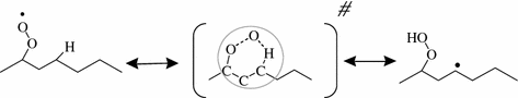
Example of isomerization in the case of radical involved in n-heptane oxidation and structure of the cyclic transition state (#)
Full size image
1. (1)
  the activation energy for hydrogen atom abstraction from the molecule by analogous radicals,
2. (2)
  the strain energy involved in the cyclic transition state.

Activation energies for isomerizations of alkyl peroxy radicals can then vary from 18 to 43 kcal/mol (Buda et al. (2005)). The rate constant proposed by Buda et al. (2005) for the reaction of Fig. 2.12 is k₁₅,_{primary-H, 6-member ring} = 5.7 × 10⁸ T exp(-12,600/T) s^–1 (1413 s^–1 at 600 K). More accurate correlations have been recently proposed based on theoretical calculations (e.g. Sharma et al. (2010), Cord et al. (2012a)).

Formation of cyclic ethers (class 23)

An example of this reaction class is shown in Fig. 2.13. The formation of oxirans, oxetanes, tetrahydrofurans, and tetrahydropyrans, containing 3, 4, 5, or 6 atoms, respectively, can be considered. In the current models (e.g. Curran et al. 1998, Ranzi et al. 2001, Buda et al. 2005), the rate constant for this type of reaction depends only on the size of the ring which is formed. However, recent work (Cord et al. 2012a) has shown the need to differentiate the type of carbon atom involved in the ring closure. The values proposed by Curran et al. (1998) for the formation of furans, the types of cyclic ethers which are formed in larger amounts as shown by experiments, is k₂₃,_furan = 9.4 × 10⁹ exp(-3.5/T) s^–1.
Fig. 2.13
Example of formation of cyclic ether in the case of radical involved in n-heptane oxidation
Full size image
Concerted eliminations (ROO· = alkene + ·HO ₂ ) (class 16))

This reaction, which was first proposed by Quelch et al. (1992), occurs via a five-membered transition state. The rate constant used by Sarathy et al. (2011) for C₇₊ alkyl radicals is that proposed by DeSain et al. (2003) for propyl radicals, i.e., k₁₆,_secondary-H = 4.3 × 10³⁶T^−7.5 exp(–17,900/T) s^–1 (377 s^–1 at 650 K) when the C–H bond broken involves a secondary hydrogen atom. As shown by the values given in previous examples, with this estimated rate constant, this reaction class can, in some cases, compete with the isomerizations leading to the branching step and then have an inhibiting effect on the oxidation of alkanes.

5 Mechanisms and Submechanisms

A detailed mechanism is not just a simple list of reactions. There is a definite structure classifying sets of reactions within the total mechanism. These subsets of reactions are called submechanisms. A large detailed mechanism can be thought of as a collection of interacting submechanisms (see Fig. 1.4 in Chap. 1). The submechanisms interact in that the initial reacting species of one submechanism are the species produced from other submechanisms. Species that are not “consumed” within one submechanism should at least be “consumed” by another submechanism. Structuring a large mechanism as the sum of many submechanisms can help in building the mechanism itself.

In a large mechanism, a modeler can focus on the individual submechanisms and their role in the entire combustion process. Under differing reactive conditions, differing submechanisms contribute different aspects of reactivity in the entire process. For example, in the combustion of large (more than four carbon atoms) hydrocarbons, a distinction is made between “high” temperature chemistry and “low” temperature chemistry producing the negative temperature coefficient behavior (see Sect. 2.3.3). For example, under high temperature conditions, species decompositions (to radicals) play a dominant role. In low temperature chemistry, additions (typically to oxygen) and recombinations can occur. In building a mechanism, if the mechanism is only to be used under high temperature conditions, only then the submechanisms which are significant under high temperatures need to be included. Those submechanisms having reactions which are significant only under low temperature conditions can be neglected. In the analysis of the mechanism (under all temperature conditions), for example, the modeler can analyze when each submechanism is significant.

The classification of submechanisms within a large mechanism can be based on several types of criteria:

Hierarchical submechanisms based on size of reactants: within a given submechanism, only species of a given size are consumed. Smaller products (produced but not consumed within this submechanism) are consumed by submechanisms ‘lower’ in the hierarchy.
Primary, secondary, and base mechanism s: it is a special case of the hierarchical structure. The primary mechanism is concerned by the reactions of the reactants and of the directly derived radicals. The secondary mechanism consumes the products of the primary mechanism. It would be possible to define iteratively tertiary and even n-ary mechanisms, but in practice in most combustion models, secondary mechanisms are designed to lead to intermediate species, which are finally consumed in a base mechanism (seed mechanism).
Pathways: It is a chain of reactions or reaction classes. The remaining species at the end of this chain should be consumed by other submechanisms.
Reaction and molecule classes: a submechanism can be classified by the reaction class it entails, for example hydrogen abstraction, or by reactant types, for example aldehydes.

5.1 Hierarchical Structure of Submechanisms

There are many ways to structure a large mechanism. One way, which is particularly useful in constructing a mechanism, is to divide the mechanism in a hierarchical structure with submechanisms including reactions for the large species build upon other submechanisms involving smaller species. In this view, a submechanism is designed with reactions to consume species of a given size (usually measured by the number of carbon atoms in the species) and to produce smaller species which, in turn, should be consumed by submechanisms lower in the hierarchy. For instance, a mechanism to model the oxidation of n-decane includes submechanisms describing the oxidation of n-nonane, n-octane, etc.

In the construction of a large mechanism, the modeler does not (or should not) construct the entire mechanism from scratch. Often, there are validated submechanisms (lower in the hierarchy) in the literature, which consume the products of the submechanisms that the modeler has designed. One example of this is in mechanism generation. Usually, the mechanisms for the larger hydrocarbons are produced automatically and the final products in these generated reactions are smaller hydrocarbons, typically with less than four carbon atoms. The submechanisms consuming these smaller hydrocarbons are not generated, but taken from the literature. This mechanism is called a base mechanism and is detailed in the next section.

5.2 Primary, Secondary, and Base Mechanisms

In one sense, this is classifying the hierarchical set of submechansims in three levels. The emphasis of the primary mechanism is generally to provide more understanding of the combustion process of the fuel. The base mechanism is usually, a well-validated detailed mechanism of smaller species, which includes reactions taken from databases, which has already been validated under the conditions being considered. The secondary mechanism can be viewed as a necessary link between the primary mechanism and the reaction base mechanism.

5.3 Pathways

Within a mechanism (or submechanism), the products of a given reaction are the reactants of another reaction. This interaction can produce a chain of reactions called a reactive pathway. This is another feature of the mechanism construction which aids not only in the building of a mechanism, but also in the understanding of the reactive process. In building a mechanism, practically speaking, it is important that the products of a reaction are consumed as reactants in other reactions. The produced species could be consumed by a significant reverse reaction. If this is not the case, during a simulation there can be an artificial, i.e., not corresponding to reality, buildup of the species concentration, i.e., a “dead-end.”

For example, in low temperature chemistry, there is an accepted pathway for the combustion of large hydrocarbons (see Fig. 2.5). An alkyl radical is produced, there is an oxygen addition followed by an intramolecular H-atom abstraction which in turn is followed by another oxygen addition which eventually leads to branching agents. In designing the mechanism, this view can be seen as a bookkeeping device, making sure that species are consumed and don’t form dead-ends. In addition, this view could be important in terms of the reduction of a mechanism through the lumping of species and reactions. Several parallel paths could be lumped into one path.

6 Varying Complexity of Combustion Mechanisms

For the simulation of more complex physical experiments, where more than the combustion chemistry is being modeled, such as burners, turbines, and engines, the complexity of detailed modeling is too high. The computational effort in chemical modeling has to give way to modeling of the physical environment. With every physical dimension or spatial detail added to a model (for example, the number of cells in a CFD calculation), complex chemical models become computationally expensive. The chemical source terms are a sub-model within a larger more computationally expensive model.

At one extreme, there are zero-dimensional calculations where large detailed mechanisms can be studied. At the other extreme there are, for example, CFD simulations which only allow the simplest of chemical models, such as global reactions or tabulations (discussed in Chap. 19). In between, there are semi-detailed and skeletal mechanisms which are often derived from detailed calculations. As a modeler, an important computational decision that has to be made is how computational much effort can be put into exploring the detailed chemistry.

In the design of a detailed mechanism, there are many modeling decisions to be made. This leads to a great diversity of possible mechanisms to describe a combustion process. One of these is how much complexity is affordable as discussed above. In the next section, some of the other factors that lead to the diversity of detailed combustion mechanisms are discussed. In the remaining sections, mechanisms of differing complexity, from large detailed to semi-detailed, and global mechanisms are presented.

6.1 Validation and Nonuniqueness of Combustion Models

The diversity in detailed kinetic mechanisms comes from a variety of sources. First and foremost is the choice of fuels, the mechanism is trying to model. As the hydrocarbon fuel gets larger, such as including more carbon atoms, or more complex, such as branched, unsaturated, oxygenated or aromatic, and species, the mechanisms contain more reactions.

Another important aspect of a constructed model is its being able to predict unknown behavior and/or to mimic known experimental behavior. A model can be “validated” if it successfully predicts known behavior. Of course, it is important to note that validation itself is not a guarantee that the model is a correct representation of reality. Several models which can be fundamentally different can produce the same result. For example, a modeler can use either an optimized global mechanism (see Sect. 2.6.4) or a detailed mechanism to match the temperature dependence of ignition delay times. Of course, the detailed mechanism will also have the potential to reproduce further data about individual species.

But if all that is needed to reproduce ignition delay time data, then the detailed model is too complex and not needed. This is a fundamental decision that a modeler has to make.

However, even two fundamentally different detailed mechanisms can match the same experimental data. How this can occur is illustrated in Fig. 2.14 which shows graphically a simple conversion path from species A through species B and C to species D. In this process (illustrated by the model labeled “Reality”), the reactions with species A as a reactant, 80 % of A is converted to A and 20 % of A is converted to B (by their respective sets of reactions). Furthermore, all of B and all of C are converted to D. In this simple model, one can conclude that all of A is converted to D. Suppose a modeler wanted to represent the conversion path from A to D with a fewer number of species. The model labeled “Significant” makes the assumption that since the majority of the conversion of A goes to C, the conversion to B can be neglected (is insignificant). This modeler assumes therefore all of A goes to C and all of C goes to D. In other words, instead of branching to both B and C, the model just neglects B and converts all to C (maybe increasing the rate to C to compensate). This model still says that all of A is converted to D, so from that viewpoint (for example, if there was no experimental evidence about species B and C), they are equivalent. The modeled labeled “Lumped” makes a different assumption, namely that the species B and C can be represented by a single “lumped” pseudo species, L. Once again from the viewpoint of A being all converted to D, this model matches the other two. If no validation data exists for species B and C, then all three models could be “correct,” i.e., give the same conversion rates from A to D.

This example shows that the potential for a number of different models, even for a very simple system as that shown in Fig. 2.14 can be quite high. In a typical combustion simulation, there can be hundreds of species, meaning that the number of conversion pathways through these species can be quite large.

Rolland and Simmie (2004), for example, compared five detailed mechanisms for methane combustion and found considerable differences.

6.2 Highly Detailed Mechanisms

Two trends of detailed mechanisms from the literature are illustrated in Fig. 2.15. The first is that with the increasing computing power that has become available over the years, larger detailed mechanisms are computationally plausible. The second trend is that larger (in terms of number carbon atoms in the species) and more complex fuels (for example number of species in the surrogate fuel, see Sect. 2.6.5) are being modeled.

In building a detailed mechanism, the modeler tries to include all the reactions and species that are “necessary.” What is necessary can be governed by matching experimental results. However, it is not necessarily possible to know whether all necessary species have been included. A good example of this is low temperature chemistry. Cool flames were being systematically studied even in the 1920s. But before the role of alkylperoxy radicals were recognized, these species, which are now an integral part of modern low temperature chemistry mechanisms, were not included. Note that the most important aspect in a detailed mechanism is not to omit any significant species or reactions. As they involve a huge number of potential free parameters, the “optimization” of detailed mechanisms in order to mimic experimental results should be kept to a minimum. However, in practice, there is always a level in detailed mechanisms where the modeler has to make a decision as to which reactions are significant and which are not, and also determine “reasonable” rate and thermodynamic constants. This often leads to a great diversity of mechanisms even for the same fuel.

6.3 Semi-Detailed and Skeletal Mechanisms

When highly detailed mechanisms are no longer computationally affordable, then the modeler has to rely on semi-detailed models or on skeletal mechanisms. While detailed mechanisms are based on fundamental reactions and try to model a wide range of conditions, skeletal mechanisms, derived from the detailed mechanisms, focus on a given chemical regime and are only valid in this regime. Skeletal reduction is typically the first step in mechanism reduction. It can be achieved through species reduction methods or by removing unimportant reactions from the detailed mechanisms. Much effort has been dedicated to the development of effective skeletal reduction techniques, as reviewed by Griffiths (1995); Tomlin et al. (1997); and Okino and Mavrovouniotis (1998); Nagy and Turanyi (2009). Chap. 17 of this book outlines these reduction techniques as follows:

Skeletal Methods:
1. 1.
  Sensitivity based methods: for example (Turányi 1990)
2. 2.
  Graph based methods for example (Lu and Law 2006, 2005)
3. 3.
  The use of optimization in model reduction
4. 4.
  Adaptive and on-the-fly reduction
.
Lumping methods leading to semi-detailed mechanisms
Chemistry-guided reduction

.

These methods have been used in the production of skeletal mechanisms such as those given in Table 2.2.

Table 2.2 A table of some skeletal mechanisms found in the literature

Full size table

6.4 Global Mechanisms

For many classes of CFD modeling, the reduction of the chemical source term has to go beyond skeletal and semi-detailed mechanisms. One class of mechanisms that accomplishes this is a “global mechanism,” a mechanism with a very limited number of species and reactions. A global mechanism is optimized either from reference detailed or semi-detailed mechanisms or directly from experimental data. Typically, they are optimized using temperature-dependent ignition delay times. There are a variety of global reaction mechanisms of different sizes (from 1 to about 20 reactions) representing a variety of reacting conditions. The size and complexity of the global mechanism a modeler chooses to use results, as with any reduced mechanism, from a compromise between relative reactive accuracy needed for the calculation, the set of conditions and the computational complexity the modeler can afford.

One of the simplest global mechanisms consists of one global reaction representing complete combustion (see Eq.(2.16)) as proposed by Westbrook and Dryer (1981). Along the same line, the two-step model (with 3 species) proposed by Selle et al. (2004):

$$ \begin{aligned} & {\text{CH}}_{ 4} + 3/ 2 {\text{O}}_{ 2} \to {\text{CO}} + 2 {\text{H}}_{ 2} {\text{O}} \\ & {\text{CO}} + 1/ 2 {\text{O}}_{ 2} = {\text{CO}}_{ 2} \\ \end{aligned} $$

(2.17)

or the four-steps model published by Jones and Lindstedt (1998), which involves also the formation of H₂, are currently used to model turbulent methane flames.

The modeling of low temperature autoignition requires larger models. The “SHELL” mechanism originally developed by Halstead et al. (1975, 1977), given in Table 2.3, is another typical example. It has eight parameterized reactions and seven pseudo species. A global mechanism scheme can be optimized to represent different reacting systems. For example, the “Fuel” in the single global reaction or the “R” in the SHELL model can represent different fuels. The SHELL model has been applied by Sazhin et al. (1999) to model the ignition delay times on n-dodecane. A modified version of the shell model was developed by Hamosfakidis and Reitz (2003) for n-heptane and tetradecane mixture and implemented into the KIVA-3 V CFD code. A series of engine simulations was then performed in order to assess its agreement with experimental data for engine applications.

Table 2.3 The basic SHELL model (Halstead et al. 1977). The reaction rates are parameterized against experimental data or a more detailed mechanism

Full size table

6.5 Surrogates: Mechanisms of Complex Fuels

A real fuel is a complex mixture of not only a large number of different types of hydrocarbon species (such as linear alkanes, branched alkanes, cyclic alkanes, and different aromatics) as can be seen in Fig. 2.2, but also encompasses a whole range of species sizes (as shown by the number of carbon atoms in the species). To formulate and then numerically calculate with a detailed mechanism describing all the chemistry of all the species in a real fuel is not practical. For this reason, the kinetic models are simplified with the definition of a “surrogate” fuel, i.e., a mixture of a “small” number of species, on the order of 2–10 species (see Table 2.3, for example) representing the properties of the complex fuel.

The standard surrogate for gasoline, which is also used in the definition of the octane reference scale, is a mixture of n-heptane and isooctane (2,2,4-trimethylpentane). The octane number is defined as 0 for n-heptane and 100 for isooctane, and it is a measure of the antiknock characteristics of gasoline. A typical surrogate for diesel is the IDEA surrogate (Hentschel et al. 1994; Lemaire et al. 2009) which is a composition of 70 % n-decane, 30 % 1-methylnapthalene (by volume). Table 2.4 lists some other examples of surrogate palette compounds making up different surrogates for different types of fuels in the literature. The table shows that the mixtures should not only contain representative molecules from all the types of molecules found in a real fuel (as shown in Fig. 1.3 of Chap. 1) but also in different ratios. With the development of detailed mechanisms with larger (more carbon atoms) and more complex (branched, cyclic, and aromatic) hydrocarbons, the surrogates can be more representative of the real fuels (Pitz and Mueller, 2011). An evaluation of gasoline surrogate components has been made by Pitz et al. (2007). A review of diesel surrogates can be found in the paper by Pitz and Mueller (2011) and a review of jet fuel surrogates can be found in the article of Dagaut and Cathonnet (2006).

Table 2.4 Some surrogate compositions for diesel and jet fuels for which models have been developed. The quantities are given is mole percent (except * which are in mass percent). The references refer to the following: 1. (Lemaire et al. 2009), 2. (Kook and Pickett, 2011), 3. (Ramirez L. et al. 2010), 4. (Mathieu et al. 2009), 5. (Mati et al. 2007), 6. (Schultz, 1991), given in italics because it is only experiments, 7. (Violi et al. 2002), 8. (Dagaut and Cathonnet, 2006), 9. (Humer et al. 2007), 10. (Natelson et al. 2008), 11. (Steil et al. 2008), 12. (Honnet et al. 2009), 13. (Dooley et al. 2010), 14. (Wang et al. 2010), 15. (Malewicki et al. 2013)

Full size table

To design an appropriate surrogate fuel, both chemical and physical comparisons have to be made between the surrogate and the real fuel. Farrell et al. (2007) in their program to develop “Fuels for Advanced Combustion Engines” (FACE) described the systematic steps toward developing a surrogate fuel:

Select the palette compounds (Mueller et al. 2012) of the surrogate fuel based on specific physical and chemical principles. Outlined below are the design considerations that must be taken into account.
Acquire the necessary elementary kinetic, thermochemical, and physical property data associated with the fuel and the surrogate.
Develop accurate predictive chemical kinetic models using the selected surrogate and gather the necessary fundamental laboratory data to validate these mechanisms.
Develop systematically reduced mechanisms based on the full detailed mechanisms, which are most likely too large to be practical in engine simulations.

To systematically accomplish the first step of deciding the candidate species for a surrogate fuel, Ranzi (2006) and Violi et al. (2002) outlined some general criteria:

Feasibility. Candidates in the surrogate must have known detailed kinetic mechanisms.
Simplicity. Mainly limited for computational capabilities to normal paraffins with <12 carbons, monocyclic paraffins with <8 carbons, and simple aromatics such as benzene, alkyl benzenes, and naphthalene.
Similarity. The surrogate is required to match real fuels in both physical and chemical properties, including (i) volatility (boiling range and flash point), (ii) sooting tendency (smoking point and luminous number), and (iii) combustion property (heat of combustion, flammability limits, and laminar premixed flame mass burning rate).
Cost and availability.

Farrell et al. (2007) and Mueller et al. (2012) outlined the “targets”; the modeler has to consider in designing a surrogate mixture which is “similar” to the real fuel. These targets are divided into three categories:

Property Targets. Similarities in fundamental physical and chemical fuel properties:
1. 1.
  density
2. 2.
  matching the hydrogen and carbon amounts
3. 3.
  gross chemical composition
4. 4.
  phase behavior (e.g., vapor–liquid equilibrium and distillation characteristics)
5. 5.
  molecular transport properties.
Development Targets. These are the kinetic and fluid dynamic processes that are important for validating surrogate mixture behavior, and that are typically evaluated in devices with better controlled conditions than those in real engines.
1. 1.
  kinetically-related phenomena (autoignition delay, burn rate, species evolution histories, emissions, etc.), with and without molecular-level transport coupling
2. 2.
  multicomponent spray vaporization
3. 3.
  droplet size distribution, and liquid penetration length
4. 4.
  experiments model validations in combustion bombs
5. 5.
  elementary kinetic studies to define specific reaction pathways.
Application Targets. obtained from engine experiments,
1. 1.
  combustion phasing and duration (timing and duration of cool flame and main heat release)
2. 2.
  combustion efficiency
3. 3.
  primary emissions (NOx, soot, CO, and unburned hydrocarbons).

Farrell et al. (2007) noted further that because the physical and chemical complexity of a surrogate fuel will be reduced, compared to that of a commercial diesel fuel, it will in general not be possible (nor necessarily desirable) to match a wide range of properties such as viscosity, chemical composition (e.g., percent aromatics), and surface tension, with a single surrogate formulation.

7 Summary

In this chapter, we have presented the essential elements related to detailed kinetic mechanisms and their use to model combustion chemistry. A purpose of this chapter was also to be an introduction to the general concepts in modeling which will be used all over this book. The use of automatic generation software to produce these detailed kinetic mechanisms is given in detail in Chap. 3. The specificities related to two particular types of biofuel, alcohols, and esters, are presented in Chap. 4. As an example of the use of semi-global mechanisms to model complex reactions, the lumped reactions used to model biomass pyrolysis and devolatilization are described in Chap. 5. Some methods to reduce the usually large size of detailed kinetic mechanisms are given in the Part IV of this book.

References

Anderlohr JM, Pires Da Cruz A, Bounaceur R et al (2010) Thermal and kinetic impact of CO, CO2, and H2O on the postoxidation of IC-engine exhaust gases. Combust Sci Technol 182:39–59
Article Google Scholar
Arrhenius S (1889) On the reaction velocity of the inversion of cane sugar by acids. Z Phys Chem 4:226
Google Scholar
Balaban AT (1985) Applications of graph theory in chemistry. J Chem Inf Comput Sci 25:334–343
Article Google Scholar
Balaban AT (1995) Chemical graphs: looking back and glimpsing ahead. J Chem Inf Com Sci 35:339–350
Article Google Scholar
Baldwin RR, Hisham MW, Walker RW (1982) Arrhenius parameters of elementary reactions involved in the oxidation of neopentane. J Chem Soc Faraday Trans I 78:1615–1627
Article Google Scholar
Battin-Leclerc F (2008) Detailed chemical kinetic models for the low-temperature combustion of hydrocarbons with application to gasoline and diesel fuel surrogates. Prog Energ Combust Sci 34:440–498
Article Google Scholar
Battin-Leclerc F, Herbinet O, Glaude PA et al (2010) Experimental confirmation of the low-temperature oxidation scheme of alkanes. Angew Chem Int Ed 49:3169–3172
Article Google Scholar
Battin-Leclerc F, Blurock E, Bounaceur R et al (2011) Towards cleaner combustion engines through groundbreaking detailed chemical kinetic models. Chem Soc Rev 40:4762–4782
Article Google Scholar
Baulch DL, Cobos CJ, Cox RA et al (1992) CEC group on evaluation of kinetic data for combustion modeling. J Phys Chem Ref Data 21:411
Article Google Scholar
Benson SW (1976) Thermochemical Kinetics, 2nd edn. John Wiley, New York
Google Scholar
Biet J, Hakka MH, Warth V et al (2008) Experimental and modeling study of the low-temperature oxidation of large alkanes. Energ Fuels 22:2258–2269
Article Google Scholar
Bloss C, Wagner V, Jenkin ME et al (2005) Development of a detailed chemical mechanism (MCMv31) for the atmospheric oxidation of aromatic hydrocarbons Atmos. Chem Phys 5:641–664
Google Scholar
Buda F, Bounaceur R, Warth V et al (2005) Progress towards a unified detailed kinetic model for the autoignition of alkanes from C₄ to C₁₀ between 600 and 1200 K. Combust Flame 142:170–186
Article Google Scholar
Byrd S, Hildreth DP (2001) Learning the functional groups: keys to success. J Chem Educ 78:1355
Article Google Scholar
Carnot S (1824) Réflexions sur la puissance motrice du feu, et sur les machines propres à développer cette puissance. Paris, Librairie Bachelier
Google Scholar
Chen W, Shuai S, Wang J (2009) A soot formation embedded reduced reaction mechanism for diesel surrogate fuel. Fuel 88:1927–1936
Article Google Scholar
Clayden J, Greeves N, Warren S (2012) Organic Chemistry, 2nd edn. Oxford University Press, USA
Google Scholar
Cord M, Sirjean B, Fournet R et al (2012a) Improvement of the modeling of the low-temperature oxidation of n-butane: study of the primary reactions. J Phys Chem A 116:6142–6158
Article Google Scholar
Cord M, Sirjean B, Fournet R et al (2012b) Study of the low temperature oxidation of propane. J Phys Chem A 116:6142–6158
Article Google Scholar
Cramer CJ (2004) Essentials of computational chemistry: theories and models, 2nd edn. Wiley, West Sussex, England
Google Scholar
Curran HJ (2006) Rate constant estimation for C₁ to C₄ alkyl and alkoxyl radical decomposition. Int J Chem Kin 28:250
Article Google Scholar
Curran HJ, Gaffuri P, Pitz WJ et al (1998) A comprehensive modeling study of n-heptane oxidation. Combust Flame 114:149–177
Article Google Scholar
Curran HJ, Gaffuri P, Pitz WJ et al (2002) A comprehensive study of iso-octane oxidation. Combust Flame 129:253–280
Article Google Scholar
Da Silva G, Bozzelli JW (2006) Enthalpies of formation, bond dissociation energies, and molecular structures of the n-aldehydes (acetaldehyde, propanal, butanal, pentanal, hexanal, and heptanal) and their radicals. J Phys Chem A 110:13058–13067
Article Google Scholar
Dagaut P, Cathonnet M (2006) The ignition, oxidation, and combustion of kerosene: a review of experimental and kinetic modeling. Prog Energ Combust Sci 32:48–92
Article Google Scholar
Davidson ER, Feller D (1986) Basis set selection for molecular calculations. Chem Rev 86:681–696
Article Google Scholar
Dec JE (2009) Advanced compression-ignition engines-understanding the in-cylinder processes. Proc Combust Inst 32:2727–2742
Article Google Scholar
DeSain JD, Klippenstein SJ, Miller JA et al (2003) Measurements, theory, and modeling of OH formation in ethyl + O₂ and propyl + O₂ reactions. J Phys Chem A 107:4415–4427
Article Google Scholar
Dooley S, Won SH, Chaos M et al (2010) A jet fuel surrogate formulated by real fuel properties. Combust Flame 157:2333–2339
Article Google Scholar
Dunnington GW, Gray J, Dohse F-E (2003) Carl Friedrich Gauss: Titan of science. The Mathematical Association of America, New York
Google Scholar
Eyring H (1935) The activated complex in chemical reactions. J Chem Phys 3:107–115
Article Google Scholar
Faraday M (1861) A course of six lectures on the chemical history of a candle. Griffin, Bohn & Co, London, UK
Google Scholar
Farrell JT, Cernansky NP, Dryer FL et al (2007) Development of an experimental database and kinetic models for surrogate diesel fuels. SAE International, Warrendale. No. 2007-01-0201
Google Scholar
Gauss CF (1823) Theoria combinationis observationum erroribus minimis obnoxiae. Gottingae, apud H Dieterich.
Google Scholar
Gilbert RG, and Smith SC (1990) Theory of unimolecular and recombination reactions. Blackwell Scientific Publication, Oxford
Google Scholar
Gillespie RJ, Robinson EA (2007) Gilbert N Lewis and the chemical bond: the electron pair and the octet rule from 1916 to the present day. J Comp Chem 28:87–97
Article Google Scholar
Goldsmith CF, Tomlin AS, Klippenstein SJ (2013) Uncertainty propagation in the derivation of phenomenological rate coefficients from theory: a case study of n-propyl radical oxidation. Proc Combust Inst 34:177–185
Article Google Scholar
Golovitchev VI, Yang J (2009) Construction of combustion models for rapeseed methyl ester bio-diesel fuel for internal combustion engine applications. Biotechnol Adv 27:641–655
Article Google Scholar
Griffiths JF (1995) Reduced kinetic models and their application to practical combustion systems. Prog Energ Combust Sci 21:25–107
Article Google Scholar
Griffiths JF, Barnard JA (1995) Flame and Combustion. 3rd ed, Chapman and Hall, London, UK
Google Scholar
Guibet JC (1999) Fuels and engines. Publications de l’Institut Français du Pétrole, Editions Technip, Paris
Google Scholar
Halstead MP, Kirsch LJ, Prothero A et al (1975) A mathematical model for hydrocarbon autoignition at high pressures. Proc Roy Soc A Mat 346:515–538
Article Google Scholar
Halstead MP, Kirsch LJ, Quinn CP (1977) The autoignition of hydrocarbon fuels at high temperatures and pressures-fitting of a mathematical model. Combust Flame 30:45–60
Article Google Scholar
Hamosfakidis V, Reitz RD (2003) Optimization of a hydrocarbon fuel ignition model for two single component surrogates of diesel fuel. Combust Flame 132:433–450
Article Google Scholar
Harding LB, Klippenstein SJ, Jasper AW (2007) Ab initio methods for reactive potential surfaces. Phys Chem Chem Phys 9:4055–4070
Article Google Scholar
Hehre WJ (2003) A guide to molecular mechanics and quantum chemical calculations wavefunction. Wavefunction, Inc. Irvine, 92612
Google Scholar
Hentschel W, Schindler KP, Haahtela O (1994) European diesel research IDEA-experimental results from DI diesel engine investigations. SAE International, Warrendale No. 941954
Book Google Scholar
Hill JG (2013) Gaussian basis sets for molecular applications. Int J Quant Chem 113:21–34
Article Google Scholar
Honnet S, Seshadri K, Niemann U et al (2009) A surrogate fuel for kerosene. Proc Combust Inst 32:485–492
Article Google Scholar
Huang C, Lu X, Huang Z (2008) New reduced chemical mechanism for homogeneous charge combustion ignition combustion investigation of primary reference fuels. Energ Fuels 22:935–944
Article Google Scholar
Hughes KJ, Halford-Maw PA, Lightfoot PD et al (1992) Direct measurements of the neo-pentyl peroxy-hydroperoxy radical isomerization over the temperature range 660–750 K. Proc Combust Inst 24:645–652
Google Scholar
Humer S, Frassoldati A, Granata S et al (2007) Experimental and kinetic modeling study of combustion of JP-8, its surrogates and reference components in laminar nonpremixed flows. Proc Combust Inst 31:393–400
Article Google Scholar
Husson B, Ferrari M, Herbinet O et al (2013) New experimental evidence and modeling study of the ethylbenzene oxidation. Proc Combust Inst 34:325–333
Article Google Scholar
Jones WP, Lindstedt RP (1988) Global reaction schemes for hydrocarbon combustion. Combust Flame 73:233–249
Article Google Scholar
Kee RJ, Rupley FM, Miller JA (1993) Chemkin II A fortran chemical kinetics package for the analysis of a gas-phase chemical kinetics Sandia Laboratories Report, SAND 89-8009B
Google Scholar
Kirsch L, Quinn C (1985) Progress towards a comprehensive model of hydrocarbon autoignition. J Chim Phys-Chim Biol 82:459–473
Google Scholar
Kook S, Pickett LM (2011) Soot volume fraction and morphology of conventional and surrogate jet fuel sprays at 1000-K and 67-MPa ambient conditions. Proc Combust Inst 33:2911–2918
Article Google Scholar
Laidler KJ (1987) Chemical kinetics, 3rd edn. Harper International, New York
Google Scholar
Lemaire R, Faccinetto A, Therssen E et al (2009) Experimental comparison of soot formation in turbulent flames of diesel and surrogate diesel fuels. Proc Combust Inst 32:737–744
Article Google Scholar
Levine IN (2000) Quantum chemistry. Pretice Hall, New Jersey, USA
Google Scholar
Levy DE (2008) Arrow-pushing in organic chemistry: an easy approach to understanding reaction mechanisms. John Wiley and Sons, Hoboken, New Jersey, USA
Google Scholar
Lewars EG (2011) Computational chemistry: introduction to the theory of molecular and quantum mechanics. 2nd edn. Springer
Google Scholar
Lewis GN (1916) The atom and the molecule. J Am Chem Soc 38:762–785
Article Google Scholar
Lu T, Law CK (2005) A directed relation graph method for mechanism reduction. Proc Combust Inst 30:1333–1341
Article Google Scholar
Lu T, Law CK (2006) Linear time reduction of large kinetic mechanisms with directed relation graph: n-heptane and iso-octane. Combust Flame 144:24–36
Article Google Scholar
Lu T, Law CK (2008) Strategies for mechanism reduction for large hydrocarbons: n-heptane. Combust Flame 154:153–163
Article Google Scholar
Lu T, Law CK (2009) Toward accommodating realistic fuel chemistry in large-scale computations. Prog Energ Combust Sci 35:192–215
Article Google Scholar
Luo YR (2003) Handbook of bond dissociation energies in organic compounds. CRC Press, Boca Raton
Google Scholar
Machrafi H, Cavadias S, Amouroux J (2009) The development and experimental validation of a reduced ternary kinetic mechanism for the auto-ignition at HCCI conditions, proposing a global reaction path for ternary gasoline surrogates. Fuel Proc Technol 90:247–263
Article Google Scholar
Malewicki T, Gudiyella S, Brezinsky K (2013) Experimental and modeling study on the oxidation of Jet A and the n-dodecane/iso-octane/n-propylbenzene/1,3,5-trimethylbenzene surrogate fuel. Combust Flame 160(17):30
Google Scholar
Mathieu O, Djebaïli-Chaumeix N, Paillard C-E et al (2009) Experimental study of soot formation from a diesel fuel surrogate in a shock tube. Combust Flame 156:1576–1586
Article Google Scholar
Mati K, Ristori A, Gaïl S et al (2007) The oxidation of a diesel fuel at 1–10 atm: experimental study in a JSR and detailed chemical kinetic modeling. Proc Combust Inst 31, 2939–2946
Google Scholar
Miller JA, Pilling MJ, Troe J (2005) Unravelling combustion mechanisms through a quantitative understanding of elementary reactions. Proc Combust Inst 30:43–88
Article Google Scholar
Mueller CJ, Cannella WJ, Bruno TJ et al (2012) Methodology for formulating diesel surrogate fuels with accurate compositional, ignition-quality, and volatility characteristics. Energ Fuels 26:3284–3303
Article Google Scholar
Nagy T, Turányi T (2009) Reduction of very large reaction mechanisms using methods based on simulation error minimization. Combust Flame 156:417–428
Article Google Scholar
Natelson RH, Kurman MS, Cernansky NP et al (2008) Experimental investigation of surrogates for jet and diesel fuels. Fuel 87:2339–2342
Article Google Scholar
Niemeyer KE, Sung C-J (2011) On the importance of graph search algorithms for DRGEP-based mechanism reduction methods. Combust Flame 158:1439–1443
Article Google Scholar
Okino MS, Mavrovouniotis ML (1998) Simplification of mathematical models of chemical reaction systems. Chem Rev 98:391–408
Article Google Scholar
Patel A, Kong S-C, Reitz RD (2004) Development and validation of a reduced reaction mechanism for HCCI engine simulations. SAE International, Warrendale. No. 2004-01-0558
Google Scholar
Peters N, Paczko G, Seiser R et al (2002) Temperature cross-over and non-thermal runaway at two-stage ignition of n-heptane. Combust Flame 128:38–59
Article Google Scholar
Pilling MJ (2009) From elementary reactions to evaluated chemical mechanisms for combustion models. Proc Combust Inst 32:27–44
Article Google Scholar
Pitz WJ, Mueller CJ (2011) Recent progress in the development of diesel surrogate fuels. Prog Energ Combust Sci 37:330–350
Article Google Scholar
Pitz WJ, Cernansky NP, Dryer FL et al (2007) Development of an experimental database and chemical kinetic models for surrogate gasoline fuels. SAE International, Warrendale. No. 2007-01-0175
Google Scholar
Pollard RT (1997) Hydrocarbons. In: Bamford CH, Tipper CFH (eds) Comprehensive chemical kinetics: gas-phase combustion, vol 17. Elsevier, Amsterdam
Google Scholar
Pretsch E, Bühlmann P, Badertscher M (2009) Structure determination of organic compounds: tables of spectral data, 4th edn. Springer, Berlin, Heidelberg
Google Scholar
Quelch GE, Gallo MM, Schaefer HF III (1992) Aspects of the reaction mechanism of ethane combustion. Conformations of the ethylperoxy radical. J Am Chem Soc 114:8239–8247
Article Google Scholar
Ramirez LHP, Hadj-Ali K, Diévart P et al (2010) Kinetics of oxidation of commercial and surrogate diesel fuels in a jet-stirred reactor: experimental and modeling studies. Energ Fuels 24:1668–1676
Article Google Scholar
Ranzi E (2006) A wide-range kinetic modeling study of oxidation and combustion of transportation fuels and surrogate mixtures. Energ Fuels 20:1024–1032
Article Google Scholar
Ranzi E, Dente M, Goldaniga A et al (2001) Lumping procedures in detailed kinetic modeling of gasification, pyrolysis, partial oxidation and combustion of hydrocarbon mixtures. Prog Energ Combust Sci 27:88–139
Article Google Scholar
Ranzi E, Frassoldati A, Granata S et al (2005) Wide-range kinetic modeling study of the pyrolysis, partial oxidation, and combustion of heavy n-alkanes. Ind Eng Chem Res 44:5170–5183
Article Google Scholar
Rolland S, Simmie JM (2004) The comparison of detailed chemical kinetic mechanisms: application to the combustion of methane. Int J Chem Kinet 36:467–471
Article Google Scholar
Sarathy SM, Westbrook CK, Mehl M et al (2011) Comprehensive chemical kinetic modeling of the oxidation of 2-methylalkanes from C7 to C20. Combust Flame 158:2338–2357
Article Google Scholar
Sazhin SS, Sazhina EM, Heikal MR et al (1999) The Shell autoignition model: a new mathematical formulation. Combust Flame 117:529–540
Article Google Scholar
Schlegel HB (1998) Geometry optimization, In: Schleyer PR, Allinger NL, Kollman PA et al (eds) Encyclopedia of computational chemistry, vol 2. Wiley, Chichester
Google Scholar
Schultz WD (1991) Oxidation products of a surrogate JP-8 fuel. ACS Petrol Chem Div Preprints 37:383
Google Scholar
Sebbar N, Bozzelli JW, Bockhorn H (2004) Thermochemical properties, rotation barriers, bond energies, and group additivity for vinyl, phenyl, ethynyl, and allyl peroxides. J Phys Chem A 108:8353–8366
Article Google Scholar
Sebbar N, Bockhorn H, Bozzelli JW (2005) Thermochemical properties, rotation barriers, and group additivity for unsaturated oxygenated hydrocarbons and radicals resulting from reaction of vinyl and phenyl radical systems with O₂. J Phys Chem A 109:2233–2253
Article Google Scholar
Selle L, Lartigue G, Poinsot T et al (2004) Compressible large eddy simulation of turbulent combustion in complex geometry on unstructured meshes. Combust Flame 137:489–505
Article Google Scholar
Semenov NN (1935) Chemical kinetics and chain reactions. The Clarendon Press, Oxford
Google Scholar
Semenov NN (1958) Some problems in chemical kinetics and reactivity. Princeton University Press, Princeton
Google Scholar
Sharma S, Raman S, Green WH (2010) Intramolecular hydrogen migration in alkylperoxy and hydroperoxyalkylperoxy radicals: accurate treatment of hindered rotors. J Phys Chem A 114:5689–5701
Article Google Scholar
Simmie JM, Black G, Curran HJ et al (2008) Enthalpies of formation and bond dissociation energies of lower alkyl hydroperoxides and related hydroperoxy and alkoxy radicals. J Phys Chem A 112:5010–5016
Article Google Scholar
Sivaramakrishnan R, Michael JV (2009) Rate constants for OH with selected large alkanes: shock-tube measurements and an improved group scheme. J Phys Chem A 113:5047–5060
Article Google Scholar
Steil U, Braun-Unkhoff M, Aigner M (2008) An experimental and modelling study on the autoignition of kerosene and surrogate fuel mixtures, 46th AIAA Aerospace Sciences Meeting and Exhibit, Aerospace Sciences Meetings American Institute of Aeronautics and Astronautics Reviews in computational chemistry, John Wiley & Sons, pp 45–81
Google Scholar
Stewart JJP (2007) Semiempirical Molecular Orbital Methods. In: Lipkowitz KB, Boyd DB (eds) Reviews in Computational Chemistry, Vol1. John Wiley & Sons, Inc., Hoboken, NJ, USA
Google Scholar
Struyf J (2009) Relating functional groups to the periodic table. J Chem Educ 86:190
Google Scholar
Strelkova MI, Safonov AA, Sukhanov LP et al (2010) Low temperature n-butane oxidation skeletal mechanism, based on multilevel approach. Combust Flame 157:641–652
Article Google Scholar
Sumathi R, Green WH (2002) Thermodynamic properties of ketenes: group additivity values from quantum chemical calculations. J Phys Chem A 106:7937–7949
Article Google Scholar
Tomlin AS, Turányi T, Pilling MJ (1997) Mathematical tools for the construction, investigation and reduction of combustion mechanisms. In: Pilling MJ (ed) Comprehensive chemical kinetics: low-temperature combustion and autoignition, vol 35. Elsevier, Amsterdam
Google Scholar
Townend DTA (1937) Ignition regions of hydrocarbons. Chem Rev 21:259–278
Article Google Scholar
Trahanovsky WS (1971) Functional groups in organic compounds. Prentice Hall, Englewood Cliffs, NJ
Google Scholar
Troe J (1974) Fall-off curves of unimolecular reaction. Ber Buns Phys Chem 78:478–488
Google Scholar
Truhlar DG, Garrett BC, Klippenstein SJ (1996) Current status of transition-state theory. J Phys Chem 100:12771–12800
Article Google Scholar
Tsang W, Hampson RF (1986) Chemical kinetic data base for combustion chemistry Part 1 Methane and related compounds. J Phys Chem Ref Data 15:1087–1279
Google Scholar
Tsurushima T (2009) A new skeletal PRF kinetic model for HCCI combustion. Proc Combust Inst 32:2835–2841
Article Google Scholar
Turányi T (1990) Sensitivity analysis of complex kinetic systems. Tools and applications. J Math Chem 5:203–248
Article MathSciNet Google Scholar
Vansteenkiste P, Van Speybroeck V, Marin GB et al (2003) Ab initio calculation of entropy and heat capacity of gas phase n-alkanes using internal rotations. J Phys Chem A 107:3139–3145
Article Google Scholar
Venot O, Hébrard E, Agùndez M et al (2012) A chemical model for the atmosphere of hot Jupiters. A&A 546:A43
Article Google Scholar
Violi A, Yan S, Eddings EG et al (2002) Experimental formulation and kinetic model for JP-8 surrogate mixtures. Combust Sci Technol 174:399–417
Article Google Scholar
Walker RW, Morley C (1997) Basic chemistry of combustion. In: Pilling MJ (ed) Comprehensive chemical kinetics: low-temperature combustion and autoignition, vol 35. Elsevier, Amsterdam
Google Scholar
Wang H, Frenklach M (1994) Transport properties of polycyclic aromatic hydrocarbons for flame modeling. Combust Flame 96:163–170
Article Google Scholar
Wang H, Warner SJ, Oehlschlaeger MA et al (2010) An experimental and kinetic modeling study of the autoignition of α-methylnaphthalene/air and α-methylnaphthalene/n-decane/air mixtures at elevated pressures. Combust Flame 157:1976–1988
Article Google Scholar
Warnatz J, Maas U, Dibble RW (2006) Combustion: physical and chemical fundamentals, modeling and simulation, experiments, pollutant formation. 4th ed, Springer, Berlin, Heidelberg
Google Scholar
Warth V, Stef N, Glaude PA et al (1998) Computed aided design of gas-phase oxidation mechanisms: Application to the modelling of normal-butane oxidation. Combust Flame 114:81–102
Article Google Scholar
Westbrook CK (2000) Chemical kinetics of hydrocarbon ignition in practical combustion systems. Proc Combust Inst 28:1563–1577
Article Google Scholar
Westbrook CK (2005) Challenges in combustion GCEP Research Symposium http://gcepstanfordedu/pdfs/uQx8GXJG882-3q6NMuyQOw/westbrook_symp05pdf
Westbrook CK, Dryer FL (1981) Simplified reaction mechanisms for the oxidation of hydrocarbon fuels in flames. Combust Sci Technol 27:31–43
Article Google Scholar
Westbrook C, Pitz W, Herbinet O et al (2009) A comprehensive detailed chemical kinetic reaction mechanism for combustion of n-alkane hydrocarbons from n-octane to n-hexadecane. Combust Flame 156:181–199
Article Google Scholar
Williams FA (1994) Combustion theory. 2nd edn. Westview Press, Boulder
Google Scholar
Yu J, Sumathi R, Green WH (2006) Accurate and efficient method for predicting thermochemistry of furans and ortho-arynes: expansion of the bond-centered group additivity method. J Phys Chem A 110:6971–6977
Article Google Scholar
Zádor J, Taatjes CA, Fernandes RX (2011) Kinetics of elementary reactions in low-temperature autoignition chemistry. Prog Energ Combust Sci 37:371–421
Article Google Scholar
Zeleznik FJ, Gordon S (1962) A general IBM 704 or 7090 computer program for computation of chemical equilibrium compositions, rocket performance, and Chapman-Jouguet detonations. NASA-TN-D-1454
Google Scholar

Download references

Acknowledgments

This work was made in the frame of COST Action CM0901. F. Battin-Leclerc thanks the European Commission (“Clean ICE” ERC Advanced Research Grant) for financial support.

Author information

Authors and Affiliations

Reaction, Lund, Sweden
Edward Blurock
Laboratoire Réactions et Génie des Procédés, CNRS, Université de Lorraine, ENSIC, 1 rue grandville, 54000, Nancy, France
Frédérique Battin-Leclerc

Authors

Edward Blurock
View author publications
You can also search for this author in PubMed Google Scholar
Frédérique Battin-Leclerc
View author publications
You can also search for this author in PubMed Google Scholar

Corresponding author

Correspondence to Frédérique Battin-Leclerc .

Editor information

Editors and Affiliations

Laboratoire Reactions et Genie des Proce, ENSIC, Nancy Cedex, France
Frédérique Battin-Leclerc
Combustion Chemistry Centre, National University of Ireland, Galway, Ireland
John M. Simmie
Department of Energy Sciences, Division, University of Lund, Lund, Sweden
Edward Blurock

Rights and permissions

Reprints and permissions

Copyright information

About this chapter

Cite this chapter

Blurock, E., Battin-Leclerc, F. (2013). Modeling Combustion with Detailed Kinetic Mechanisms. In: Battin-Leclerc, F., Simmie, J., Blurock, E. (eds) Cleaner Combustion. Green Energy and Technology. Springer, London. https://doi.org/10.1007/978-1-4471-5307-8_2

Download citation

DOI: https://doi.org/10.1007/978-1-4471-5307-8_2
Published: 06 September 2013
Publisher Name: Springer, London
Print ISBN: 978-1-4471-5306-1
Online ISBN: 978-1-4471-5307-8
eBook Packages: EnergyEnergy (R0)

Publish with us

Policies and ethics

Modeling Combustion with Detailed Kinetic Mechanisms

Abstract

Similar content being viewed by others

Structural analysis of combustion mechanisms

Unsteady Combustion Processes Controlled by Detailed Chemical Kinetics

Reduced Kinetic Models for Methane Flame Simulations

Keywords

1 Introduction

2 Chemical Combustion Models

2.1 Generalities About Chemical Mechanisms

2.2 Detailed Chemical Mechanisms

2.3 Low and High Temperature Detailed Chemical Combustion Mechanisms

3 Species and Molecular Representation

3.1 Molecular Representations in Detailed Mechanisms

3.2 Lewis Structures and Detailed Combustion Modeling

3.3 Functional Groups

3.4 Molecular Representation and Reactivity

4 Reactions

4.1 Concept of Reaction Classes

4.2 List of Reaction Classes Usually Used in Combustion Mechanisms

4.3 Kinetic Data of the Reaction Classes Used in Combustion Mechanisms

5 Mechanisms and Submechanisms

5.1 Hierarchical Structure of Submechanisms

5.2 Primary, Secondary, and Base Mechanisms

5.3 Pathways

6 Varying Complexity of Combustion Mechanisms

6.1 Validation and Nonuniqueness of Combustion Models

6.2 Highly Detailed Mechanisms

6.3 Semi-Detailed and Skeletal Mechanisms

6.4 Global Mechanisms

6.5 Surrogates: Mechanisms of Complex Fuels

7 Summary

References

Acknowledgments

Author information

Authors and Affiliations

Corresponding author

Editor information

Editors and Affiliations

Rights and permissions

Copyright information

About this chapter

Cite this chapter

Download citation

Share this chapter

Publish with us

Search

Navigation