
Abstract
Background
Dynamics modeling and control of the electric vehicles (EV) in regenerative braking process are feasible for energy reservation.
Method
To recover more energy and ensure braking safety in the regenerative braking process, dynamic model of EV in braking process has been established. Besides, a braking force distribution strategy, discussing the relationship between the relationship curve between braking forces of the front and the rear wheels (the F curve) and the Economic Commission for Europe (ECE) curve, is proposed based on the desired force distribution curve (I curve) and ECE curve. In addition, the fuzzy logic regulations between braking force and the braking requirements, vehicle velocity, and battery SOC are established which can ensure driving safety and battery safety simultaneously. The proposed control strategies are performed efficiently in ensuring driving safety, comfort, stability, and battery safety of EV by employed Hardware In-the-Loop (HIL) simulation.
Result
The total energy usage efficiency of EV can be improved about 10% and the one-time charging mileage of EV is prolonged.
Conclusion
The new control strategy is feasible in recovering more energy in the braking process.
Introduction
Vehicle, as the mainstay of the world’s economy, is also one of the most important transportations for human beings. However, the great increase of vehicle applications inevitably leads to the problems of energy shortage and environmental problems such as climate changes and global warming [1, 2]. Recently, the regenerative braking is one of the most effective ways to improve energy economy of EVs [3]. Prius developed by TOYOTA can recycle about 23% energy using the regenerative braking system. In city cycle, 50% of the total energy provided by motors is consumed by brakes, but about 80% braking energy can be recovered, which means that about 40% energy of all the energy can be recycled theoretically [4].
To ensure the braking safety or to recover more energy from the braking, many researchers and institutions have done a lot of work on the law of braking force distribution, and have made great achievements [5, 6]. Among them, some researchers are committed to ensuring safety of the braking. In [7], when the ratio of electromotive force to mechanical braking force is 4–1, the motor can supply enough braking torque at any velocity. According to the braking strength, Lian et al. [8] divided the Regenerative Braking Force (RBF) distribution strategy into three grades, and a braking torque distribution regulation according to the continuity of regenerative braking strength was proposed to ensure safety. The method is that the tractor rear, the trailer, and the tractor front wheel slips decreased in order [9]. In this paper, the slip ratio was considered adequately to ensure braking safety, but cannot ensure recycle more energy. In [10], a ratio k is introduced to redistribute the braking force which will affect the braking force. The principle to optimize the performance of the strategy is the wheels slip ratio and the motor loss. The optimal distribution regulation only depends on the vehicle velocity and acceleration. In the literature [11], the ratio of the driving force distribution for reducing the input energy of the inverter was generated with considering load transfer and motor losses. The proposed method is effective on various driving states such as constant velocity, acceleration, and deceleration due to the distribution regulation only based on vehicle speed and acceleration, which is not required for pre-computation and control. By applying the hydraulic braking force on the front wheels less than the baseline control method and the RBF applied on the rear wheels, a modified regenerative braking control method was presented in the literature [11] that helps to improve the regeneration efficiency. On average, a force distribution strategy based on the tire dynamic load and the minimum objective function was proposed to control the motor and the RBF to ensure the braking stability [12]. In paper [13], an optimal force distribution method was proposed for EV which has four wheel motors independently to improve vehicle safety. To improve the recycling efficiency of the regenerated brake energy in hybrid electric vehicle, the control strategy according to the maximum braking torque recovery is proposed [14]. However, the regenerative braking torque depends on the front wheel-braking curve; therefore, the maximum braking energy cannot be ensured. By the way of yaw velocity error feedback, the front–rear force distribution can be changed. Besides, the purpose of maintaining vehicle path and maximizing acceleration was achieved through the left–right lateral acceleration error feedback [15]. Based on the force distribution regulation, a brake control method was presented to improve comfortable sensation in the braking. According to the phase plane theory, an optimal brake force is obtained for ABS control of an EV and an RBS control method named “serial control strategy” is designed for EVs during anti-lock braking process [16]. Based on the wheel slips, a braking force distribution method was proposed to improve braking stability under different deceleration levels in [13]. However, this force distribution method proposed above mainly focuses on ensuring braking safety while cannot recover as much energy as possible, or even ignoring the problem of energy recovery in the braking process. Finally, the experiment set-up, which has four types of tire–road adhesion ratio, is established and the testing result shows effectiveness of the control method.
In addition, in the design of force distribution strategy, many researchers pay more attention to ensure braking energy, but fail to take full account of safety problems. For instance, according to the quality of the motor, Gao [17] proposed a control method based on the maximum motor braking torque curve. However, this method may cause safety issue to the vehicles due to other factors such as the slip ratio and the State of Charge (SOC) which are not sufficiently considered. In paper [18], a regenerative braking force controller (RBFC) was designed. This is a special case of brake force distribution, which mainly focuses on the ensuring stability operation in the swerve period. Therefore, it is only applicable to small turning and slip coefficients and other cases are not discussed in this paper. In [19], taking into account the SOC and car speed included by the weight factor to determine the regeneration braking force, it is allocated among vehicle wheels evenly to regenerate more energy from the braking. However, only SOC and vehicle speed are considered in the braking strategy, so braking safety cannot be guaranteed. Considering the requirements of the power and maximum speed of motor and the stability of vehicles, a braking force distribution strategy was proposed in [20] for maximum recovering of energy at the expense of ensuring the safety of vehicles.
Through all the references above, the demands of the braking safety and the energy conversation cannot always be satisfied simultaneously. In 1999, Gao and Ehsani [21] proposed the “ideal” distribution equation of the braking torques among vehicle axles to ensure the driving safety. On the basis of this theory, Li Peng [22] developed a regenerative braking strategy that if the adhesion coefficient is large enough, the distribution ratio will follow the desired curve. However, this method cannot clearly distinguish the value of the adhesion coefficient. Thereafter, Zou [23] put forward an improved force distribution law, which is applicable to various adhesive coefficients. However, it is difficult to choose the appropriate adjustment curve. In [24], based on the ECE distribution regulation, the RBF distribution can generate maximum regenerative braking torque, and energy recovery maximization can be achieved compared with ideal distribution of the braking force and speed regulation. Zhang, et al. [25], obtained the braking torque based on the I curve, while complying with ECE curves. Besides, the method is realized by the interpolation via offline optimization information. Through simulation results, it demonstrates that the force allocation scheme proposed in the paper can recover more energy in the braking. In [26], a force distribution method was presented. When the vertical loads of vehicle wheels are known, the front- and rear-braking forces follow the I curve. When the vertical wheel loads cannot be measured, the actual braking force curve would locate between the unloaded ideal braking force distribution curve and the minimum rear wheel-braking force limitation curve. However, this method cannot ensure regenerate as much more energy as possible. In [27], excess brake force was distributed driven wheels. In the braking distribution regulation design process, it is desirable to recover as much energy as possible for improving the driving range and fuel economy. However, with respect to vehicle behavior, the brake force distribution would increasingly deviate from the ideal curve as the amount of energy regenerated increases, and the cornering force would decrease accordingly.
In addition, selection and design of reasonable control strategy are also the focus of current research. In [28], the DP control method was used to distribute energy and the hierarchical control strategy is used in [29] to decide the optimal downshift point, and cooperate control of regenerative and hydraulic braking. SOCmax, SOCmin, SOChigh, and SOClow were set 0.65, 0.25, 0.60, and 0.30, respectively. Gao et al. [30] introduced the neural network to calculate the value of RBF. In practical industry, the safety, reliability, and ease applications are the main performance indicators. Therefore, the fuzzy logic control has attracted more attentions of researchers in the field of regenerative braking. Yao [31] designed a motor torque controller based on the Mamdani’s fuzzy controller. However, it only takes the pedal and speed into consideration to determine the RBF. Zhang [32] presented a fuzzy controller including two inputs batteries’ SOC and a special parameter P defined by the torque input and the maximum torque of the motor. However, this method only considers vehicle velocity and motor’s achievable force, but without the maximum allowed charging current of the battery. Li [33] proposed a fuzzy control logic controller including the braking pedal and the motor speed. In [34], an estimation algorithm of the tire–road friction based on the fuzzy logic was proposed and used in BFD control strategy, which introduces the longitudinal wheel slip measured by acceleration and speed sensors. The algorithm is integrated in the controller which can improve the braking energy recovery. In controller [35], it only considers the front braking force, the SOC, and the EV speed as input. From the references listed above, the fuzzy logic is an effective method in the regenerative braking system design.
Therefore, a fuzzy logic-based regenerative braking controller is proposed. To improve energy efficiency and braking safety, a force redistribution regulation among the front-mechanical, the rear-mechanical, and the RBFs is obtained. Besides, the RBFC designed in the paper includes the braking requirement and the car velocity related to braking safety, also considers the factors such as the battery SOC and temperature, which are important to ensure the battery safety. Furthermore, an HIL simulation experiment set-up and the simulation model system are established to validate the proposed strategy.
In the next section, basic components and working principles of the regenerative braking system are introduced followed by which the force redistribution regulation of the EV will be presented. Next, the fuzzy logic-based controller is designed to realize the regenerative braking control. An HIL experimental platform, which is used to validate the method, is explained in the subsequent section. Before the concluding section, the performance of the method in ensuring braking safety and energy conservation is given. Conclusions are summarized in the last section.
Dynamic model of EV in braking process
Preliminaries of regenerative braking
The regenerative braking system of EV can be seen in Fig. 1. According to the driving requirements, the driver treads on brake pedal. The angle senor which measures inclination of the pedal will send the driver’s driving demands to the fuzzy controller. According to the controller, the braking forces can be obtained.

Braking system of EV
Dynamic analysis of vehicle in braking process
The force analysis of EV during braking is revealed in Fig. 2. When ignoring the deceleration, the rotating mass generates the roll resistance couple moment, the air resistance, and inertia coupling. Besides, in the following analysis, the rolling and slipping process during braking is neglected, and the adhesion coefficient is constant φ0 [36].

Force analysis of vehicle
Taking the contacting points of the front wheels and the rear wheels as research objects, the moment can be calculated from Eqs. (1) and (2):
Rear wheels:
Front wheels:
where Fzf, Fzr are forces applied to vehicle by the surface, respectively; G is the vehicle weight, G = mg, and m is the vehicle mass; hg is the distance between the gravity center and the surface; c, b are the distance between the front axles, the rear axles, and the gravity center, respectively; L is the distance between the vehicle axles; Fj is the inertia force during braking. It equates to Fj = m×dv/dt = ma; herein, v is the car speed and a is the acceleration.
The adhesion coefficients are different with different loads. We assume that all the wheels are locked, and then, the vehicle will remain in pure sliding state, Fxf = Fxr = Gφ, as the forces applied to the vehicle are equal: Fj = m × dv/dt = Fxf = Fxr = Gφ, so, dv/dt = φg.
From Eqs. (1) and (2), we can obtain the forces applied to vehicle by the surface are as follows:
Basement of the Force Distribution Regulation
The meaning and analysis of all braking forces distribution curves can be seen from Fig. 3. I curve indicates the ideal distribution of front and rear wheels, and its can be calculated by the equation as follows:

Braking force distribution
where Ff, Fr are the front and the rear wheel-braking forces.
ECE curve [37] means the command curve of braking forces between front and rear wheels of two-axle vehicle, drawn up by the European commercial committee of UN, and the vehicles satisfy \( z \ge 0.1 + 0.85(\phi - 0.2) \), with 0.2 < φ < 0.8, and then, calculation equation of ECE curve can be written as follows:
where z is the braking severity, and its calculation equation is defined as z = j/g [38].
F curve [38] is the relationship curve between braking force of front and rear wheels. As the front wheels locked, the rear wheels are unlocked on the roads with different φ:
where Ff, Fr are the front and rear wheels braking forces when all of them are locked, respectively.
According to the braking pedal, the braking force distribution curve is obtained and the calculation equation as follows:
where F means the REquired Braking Force (REBF) of driver.
Calculation of Braking Force in the Braking
In the process of braking, the driver will push the pedal down to different angles according to driving conditions and required braking commands. The relationship between brake pedal angle and braking force is proportionate. Herein, assuming that the ratio is k, then F = kα, α is the brake pedal angle (0° ≤ α ≤ 90°); k is different depending on the type of vehicle that can be estimated from experiments.
Calculation of the Maximum Braking Force
According to the relationships of the capacity of batteries, SOC, SOH, temperature, conformity, and the motor braking force, we obtain the algorithm flowchart Fig. 4 as follows.

Motor braking force control algorithm flowchart
Force Distribution Regulation Design
At present, the purpose of the regenerative braking strategy is increasing the electric one to produce more energy. On most occasions, the current generated by electrical braking force cannot be totally regenerated for restrictions of batteries and so on. At the same time, the charging current can cause damage to batteries if it is larger than the permitted maximum charging current, and the braking safety, comfort, and stability will also be decreased. To solve these problems, we introduce the maximum braking force Fm into the distribution strategy, which has the advantage of regenerating as much energy as possible and improve the braking safety, comfort and safety in emergency braking. The force distribution among the vehicle wheels can be divided into the following two conditions.
The F Curve and the ECE Curve are Tangent or Disjoint
-
(1)
When FB ≥ FA, the front–rear wheel force distributions can be shown as the thick curve of Fig. 5a. In the figure, at the OA stage, all the force is only generated by motor due to the braking force is small; at the AC stage, with the increment of braking force required by vehicle, both the electrical force and mechanical force of rear wheels have contribution to generate braking force; Then, at the CD stage, the braking force can be provided by mechanical force and electrical force of the vehicle wheels to ensure safety of the vehicle, owing to the requirements of large braking force and deceleration. The relationships of force distribution can be calculated by Eqs. (9–11).
Fig. 5 
The F curve and the ECE curve are tangent or disjoint
If F ≤ Fm1 then
$$ \left[ {F_{\text{f}} ,F_{\text{r}} } \right] = \left[ {F,0} \right]. $$(9)If \( F_{\text{m1}} < F \le {{G\left[ {\sqrt {b^{2} + 4 \times h_{\text{g}} \times {L \mathord{\left/ {\vphantom {L G}} \right. \kern-0pt} G}} F_{\text{m1}} - b} \right]} \mathord{\left/ {\vphantom {{G\left[ {\sqrt {b^{2} + 4 \times h_{\text{g}} \times {L \mathord{\left/ {\vphantom {L G}} \right. \kern-0pt} G}} F_{\text{m1}} - b} \right]} {h_{\text{g}} }}} \right. \kern-0pt} {h_{\text{g}} }} \), then
$$ \left[ {F_{\text{f}} ,F_{\text{r}} } \right] = \left[ {F_{{{\text{m}}1}} ,F - F_{{{\text{m}}1}} } \right]. $$(10)If \( \frac{1}{2}\frac{G}{{h_{\text{g}} }}\left[ {\sqrt {b^{2} + \frac{{4h_{g} L}}{G}} F_{{{\text{m}}1}} - b} \right] < F \le (A + B) \), then
$$ \left[ {F_{\text{f}} ,F_{\text{r}} } \right] = 2{{\left( {F + G \times {b \mathord{\left/ {\vphantom {b {2 \times h_{\text{g}} }}} \right. \kern-0pt} {2 \times h_{\text{g}} }}} \right)} \mathord{\left/ {\vphantom {{\left( {F + G \times {b \mathord{\left/ {\vphantom {b {2 \times h_{\text{g}} }}} \right. \kern-0pt} {2 \times h_{\text{g}} }}} \right)} G}} \right. \kern-0pt} G}{{\sqrt {b^{2} + 4 \times h_{\text{g}} \times {L \mathord{\left/ {\vphantom {L G}} \right. \kern-0pt} G}} } \mathord{\left/ {\vphantom {{\sqrt {b^{2} + 4 \times h_{\text{g}} \times {L \mathord{\left/ {\vphantom {L G}} \right. \kern-0pt} G}} } {h_{\text{g}} }}} \right. \kern-0pt} {h_{\text{g}} }},F - {{2\left( {F + G \times {b \mathord{\left/ {\vphantom {b 2}} \right. \kern-0pt} 2} \times h_{\text{g}} } \right)} \mathord{\left/ {\vphantom {{2\left( {F + G \times {b \mathord{\left/ {\vphantom {b 2}} \right. \kern-0pt} 2} \times h_{\text{g}} } \right)} G}} \right. \kern-0pt} G}{{\sqrt {b^{2} - 4 \times h_{\text{g}} {L \mathord{\left/ {\vphantom {L G}} \right. \kern-0pt} G}} } \mathord{\left/ {\vphantom {{\sqrt {b^{2} - 4 \times h_{\text{g}} {L \mathord{\left/ {\vphantom {L G}} \right. \kern-0pt} G}} } {h_{\text{g}} }}} \right. \kern-0pt} {h_{\text{g}} }}, $$(11)$$ {\text{where}}\;A = {{\frac{Gb}{{2h_{\text{g}} }}} \mathord{\left/ {\vphantom {{\frac{Gb}{{2h_{\text{g}} }}} {\left[ {\frac{{L - \varphi h_{\text{g}} }}{{\varphi h_{\text{g}} }} - \frac{G}{{2h_{\text{g}} }}\sqrt {b^{2} + \frac{{4h_{\text{g}} L}}{G}} + 1} \right]}}} \right. \kern-0pt} {\left[ {\frac{{L - \varphi h_{\text{g}} }}{{\varphi h_{\text{g}} }} - \frac{G}{{2h_{\text{g}} }}\sqrt {b^{2} + \frac{{4h_{\text{g}} L}}{G}} + 1} \right]}};B = \frac{1}{2}\left[ {\frac{G}{{h_{g} }}\sqrt {b^{2} + \frac{{4h_{g} L}}{G}} F_{{{\text{m}}1}} - \left( {\frac{Gb}{{h_{\text{g}} }} + 2F_{{{\text{m}}1}} } \right)} \right]. $$ -
(2)
In the second cases, FB ≤ FA, FB ≤ FH, and FC ≤ FD, the redesigned force distribution regulation of the vehicle wheels is shown in Fig. 5b, c. At the OB stage, the braking force of vehicle is only provided by motor; at the BP stage, the braking force can be generated by electrical force and mechanical force of rear wheels based on the regulation of maximum motor torque curve; At the CD stage, the braking force is generated by electrical force and mechanical forces of the vehicle wheels. The relationships can be presented in Eqs. (12–15)
If \( F \le \frac{Gb\varphi }{{\left( {L - \varphi h_{\text{g}} } \right)}} \), then
$$ \left[ {F_{\text{f}} ,F_{\text{r}} } \right] = \left[ {F,0} \right] $$(12)If \( \frac{Gb\varphi }{{\left( {L - \varphi h_{\text{g}} } \right)}} < F \le \left( {\frac{{F_{{{\text{m}}1}} L}}{{\varphi h_{\text{g}} }} - \frac{Gb}{{h_{\text{g}} }}} \right) \), then
$$ \left[ {F_{\text{f}} ,F_{\text{r}} } \right] = \left[ {\frac{{\varphi h_{\text{g}} }}{L}\left( {F + \frac{Gb}{{h_{\text{g}} }}} \right),\left( {1 - \frac{{\varphi h_{\text{g}} }}{L}} \right)F + \frac{\varphi Gb}{L}} \right]. $$(13)If \( \left( {\frac{{F_{{{\text{m}}1}} L}}{{\varphi h_{\text{g}} }} - \frac{Gb}{{h_{\text{g}} }}} \right) < F \le \frac{G}{{2h_{\text{g}} }}\left( {\sqrt {b_{2} + \frac{{4h_{\text{g}} L}}{G}} F_{{{\text{m}}1}} - 1} \right) \), then
$$ \left[ {F_{\text{f}} ,F_{\text{r}} } \right] = \left[ {F_{{{\text{m}}1}} ,F - F_{{{\text{m}}1}} } \right] $$(14)If \( \frac{G}{{2h_{\text{g}} }}\left( {\sqrt {b_{2} + \frac{{4h_{\text{g}} L}}{G}} F_{{{\text{m}}1}} - 1} \right) < F \le (A + B) \) then
$$ \left[ {F_{\text{f}} ,F_{\text{r}} } \right] = \left[ {{{2\left( {F + \frac{Gb}{{2h_{\text{g}} }}} \right)} \mathord{\left/ {\vphantom {{2\left( {F + \frac{Gb}{{2h_{\text{g}} }}} \right)} {\frac{G}{{h_{\text{g}} }}\sqrt {b^{2} + \frac{{4h_{\text{g}} L}}{G}} ,F - {{2\left( {F + \frac{Gb}{{2h_{\text{g}} }}} \right)} \mathord{\left/ {\vphantom {{2\left( {F + \frac{Gb}{{2h_{\text{g}} }}} \right)} {\left( {\frac{G}{{h_{\text{g}} }}\sqrt {b^{2} - \frac{{4h_{\text{g}} L}}{G}} } \right)}}} \right. \kern-0pt} {\left( {\frac{G}{{h_{\text{g}} }}\sqrt {b^{2} - \frac{{4h_{\text{g}} L}}{G}} } \right)}}}}} \right. \kern-0pt} {\frac{G}{{h_{\text{g}} }}\sqrt {b^{2} + \frac{{4h_{\text{g}} L}}{G}} ,F - {{2\left( {F + \frac{Gb}{{2h_{\text{g}} }}} \right)} \mathord{\left/ {\vphantom {{2\left( {F + \frac{Gb}{{2h_{\text{g}} }}} \right)} {\left( {\frac{G}{{h_{\text{g}} }}\sqrt {b^{2} - \frac{{4h_{\text{g}} L}}{G}} } \right)}}} \right. \kern-0pt} {\left( {\frac{G}{{h_{\text{g}} }}\sqrt {b^{2} - \frac{{4h_{\text{g}} L}}{G}} } \right)}}}}} \right], $$(15)$$ {\text{where}}\;A = {{\frac{G}{{2h_{\text{g}} }}} \mathord{\left/ {\vphantom {{\frac{G}{{2h_{\text{g}} }}} {\left[ {\frac{{L - \varphi h_{\text{g}} }}{{\varphi h_{\text{g}} }} - \frac{G}{{2h_{\text{g}} }}\sqrt {b^{2} + \frac{{4h_{\text{g}} L}}{G}} { + }1} \right]}}} \right. \kern-0pt} {\left[ {\frac{{L - \varphi h_{\text{g}} }}{{\varphi h_{\text{g}} }} - \frac{G}{{2h_{\text{g}} }}\sqrt {b^{2} + \frac{{4h_{\text{g}} L}}{G}} { + }1} \right]}};\,B = \frac{1}{2}\left[ {\frac{G}{{h_{\text{g}} }}\sqrt {b^{2} + \frac{{4h_{\text{g}} L}}{G}} F_{{{\text{m}}1}} - \left( {\frac{Gb}{{h_{\text{g}} }} + 2F_{\text{m1}} } \right)} \right]. $$ -
(3)
When FA ≥ FB, FH ≥ FB and FC ≥ FD, the front–rear wheel force distributions are shown as the thick curves in Fig. 5d, e. At the OB stage, the braking force of vehicle is only generated by motor; at the BD stage, and the braking force is generated by electrical force and mechanical force wheels of rear wheels based on the F curve. The relationships can be expressed as Eqs. (16) to (17).
If \( F \le \frac{Gb\varphi }{{\left( {L - \varphi h_{\text{g}} } \right)}} \), then
$$ \left[ {F_{\text{f}} ,F_{\text{r}} } \right] = \left[ {F,0} \right]. $$(16)If \( \frac{Gb\varphi }{{\left( {L - \varphi - g} \right)}} < F \le (A + B) \), then
$$ [F_{\text{f}} ,F_{\text{r}} ] = \left[ {\frac{\varphi }{L}\left[ {Fh_{\text{g}} + Gb} \right],F - \frac{\varphi }{L}\left( {Fh_{g} + Gb} \right)} \right] $$(17)$$ {\text{where}}\;A = {{\frac{G}{{2h_{\text{g}} }}} \mathord{\left/ {\vphantom {{\frac{G}{{2h_{\text{g}} }}} {\left[ {\frac{{L - \varphi h_{\text{g}} }}{{\varphi h_{\text{g}} }} - \frac{G}{{2h_{\text{g}} }}\sqrt {b^{2} + \frac{{4h_{\text{g}} L}}{G}} { + }1} \right]}}} \right. \kern-0pt} {\left[ {\frac{{L - \varphi h_{\text{g}} }}{{\varphi h_{\text{g}} }} - \frac{G}{{2h_{\text{g}} }}\sqrt {b^{2} + \frac{{4h_{\text{g}} L}}{G}} { + }1} \right]}};B = \frac{1}{2}\left[ {\frac{G}{{h_{\text{g}} }}\sqrt {b^{2} + \frac{{4h_{g} L}}{G}} F_{{{\text{m}}1}} - \left( {\frac{Gb}{{h_{\text{g}} }} + 2F_{{{\text{m}}1}} } \right)} \right]. $$

The F Curve and the ECE Curve are Intersect
-
(1)
When FA ≤ FH, the front–rear wheel force distributions will follow the thick curve showing in Fig. 6a. At the OA stage, the vehicle braking force can be calculated by Eq. (18); at the AC stage, the estimation equation of braking force is presented as (19) that is generated by electrical force and mechanical force of rear wheels with the increment of braking force required by vehicle; At the CD stage, Eq. (20) is used to calculate the braking force, which is provided by electrical and mechanical forces of the vehicle wheels.
Fig. 6 
The F curve and the ECE curve are intersect
If F ≤ Fm1, then
$$ \left[ {F_{\text{f}} ,F_{\text{r}} } \right] = \left[ {F,0} \right]. $$(18)If \( F_{\text{m1}} < F \le \frac{1}{2}\left[ {\frac{G}{{h_{\text{g}} }}\sqrt {b^{2} + \frac{{4h_{\text{g}} L}}{G}} F_{\text{m1}} - \left( {\frac{Gb}{{h_{\text{g}} }} + 2F_{\text{m1}} } \right)} \right]F_{\text{m1}} \), then
$$ \left[ {F_{\text{f}} ,F_{\text{r}} } \right] = \left[ {F_{{{\text{m}}1}} ,F - F_{{{\text{m}}1}} } \right]. $$(19)If \( \frac{1}{2}\left[ {\frac{G}{{h_{\text{g}} }}\sqrt {b^{2} + \frac{{4h_{\text{g}} L}}{G}} F_{\text{m1}} - \left( {\frac{Gb}{{h_{\text{g}} }} + 2F_{\text{m1}} } \right)} \right] < F \le (A + B) \), then
$$ \left[ {F_{\text{f}} ,F_{\text{r}} } \right]{ = }\left[ {{{2\left( {F + \frac{Gb}{{2h_{\text{g}} }}} \right)} \mathord{\left/ {\vphantom {{2\left( {F + \frac{Gb}{{2h_{\text{g}} }}} \right)} {\frac{G}{{h_{\text{g}} }}\sqrt {b^{2} + \frac{{4h_{\text{g}} L}}{G}} ,F - {{2\left( {F + \frac{Gb}{{2h_{\text{g}} }}} \right)} \mathord{\left/ {\vphantom {{2\left( {F + \frac{Gb}{{2h_{\text{g}} }}} \right)} {\left( {\frac{G}{{h_{\text{g}} }}\sqrt {b^{2} - \frac{{4h_{\text{g}} L}}{G}} } \right)}}} \right. \kern-0pt} {\left( {\frac{G}{{h_{\text{g}} }}\sqrt {b^{2} - \frac{{4h_{\text{g}} L}}{G}} } \right)}}}}} \right. \kern-0pt} {\frac{G}{{h_{\text{g}} }}\sqrt {b^{2} + \frac{{4h_{\text{g}} L}}{G}} ,F - {{2\left( {F + \frac{Gb}{{2h_{\text{g}} }}} \right)} \mathord{\left/ {\vphantom {{2\left( {F + \frac{Gb}{{2h_{\text{g}} }}} \right)} {\left( {\frac{G}{{h_{\text{g}} }}\sqrt {b^{2} - \frac{{4h_{\text{g}} L}}{G}} } \right)}}} \right. \kern-0pt} {\left( {\frac{G}{{h_{\text{g}} }}\sqrt {b^{2} - \frac{{4h_{\text{g}} L}}{G}} } \right)}}}}} \right], $$(20)$$ {\text{where}}\;A = {{\frac{G}{{2h_{\text{g}} }}} \mathord{\left/ {\vphantom {{\frac{G}{{2h_{\text{g}} }}} {\left[ {\frac{{L - \varphi h_{\text{g}} }}{{\varphi h_{\text{g}} }} - \frac{G}{{2h_{\text{g}} }}\sqrt {b^{2} + \frac{{4h_{\text{g}} L}}{G}} { + }1} \right]}}} \right. \kern-0pt} {\left[ {\frac{{L - \varphi h_{\text{g}} }}{{\varphi h_{\text{g}} }} - \frac{G}{{2h_{\text{g}} }}\sqrt {b^{2} + \frac{{4h_{\text{g}} L}}{G}} { + }1} \right]}};B = \frac{1}{2}\left[ {\frac{G}{{h_{\text{g}} }}\sqrt {b^{2} + \frac{{4h_{\text{g}} L}}{G}} F_{\text{m1}} - \left( {\frac{Gb}{{h_{\text{g}} }} + 2F_{\text{m1}} } \right)} \right]. $$ -
(2)
When FB ≥ FA ≥ FH, the front–rear wheel force distributions are presented in Fig. 6b with the thick curve. At the OH stage, the braking force of vehicle can be only provided by motor and its calculation equation is written as (21); At the HP stage, according to the standard of ECE braking force regulation, the force distribution regulation is the same as ECE [see Eq. (22)]; At the CP stage, with the increment of braking force required by vehicle, electrical braking force reaches the maximum, and its distribution can be expressed in Eq. (23); At the CD stage, based on Eq. (24), get the braking force, and both the electrical and mechanical forces and rear wheels have contributed to the force to ensure the safety of the vehicle.
If \( F \le Gz = G \times \left[ {0.1 + 0.85\left( {\varphi - 0.2} \right)} \right] = G \times 0.1 \), then
$$ \left[ {F_{\text{f}} ,F_{\text{r}} } \right] = \left[ {F,0} \right] $$(21)If \( 0.1G < F \le G{{(0.07G - 0.85LbF_{\text{m1}} )} \mathord{\left/ {\vphantom {{(0.07G - 0.85LbF_{\text{m1}} )} {(0.85LbF_{\text{m1}} - G)}}} \right. \kern-0pt} {(0.85LbF_{\text{m1}} - G)}} \), then
$$ \left[ {F_{\text{f}} ,F_{\text{r}} } \right]{ = }\left[ {\frac{z + 0.07}{0.85}\frac{G}{L}\left( {b + zh_{\text{g}} } \right),Gz - \frac{z + 0.07}{0.85}\frac{G}{L}\left( {b + zh_{\text{g}} } \right)} \right]. $$(22)If \( G{{(0.07G - 0.85LbF_{{{\text{m}}1}} )} \mathord{\left/ {\vphantom {{(0.07G - 0.85LbF_{{{\text{m}}1}} )} {(0.85Lh_{\text{g}} F_{\text{m1}} - G)}}} \right. \kern-0pt} {(0.85Lh_{\text{g}} F_{\text{m1}} - G)}} < F \le \frac{1}{2}\left[ {\frac{G}{{h_{\text{g}} }}\sqrt {b^{2} + \frac{{4h_{\text{g}} L}}{G}} F_{\text{m1}} - \left( {\frac{Gb}{{h_{\text{g}} }} + 2F_{\text{m1}} } \right)} \right]{ + }F_{\text{m1}} \), then
$$ \left[ {F_{\text{f}} ,F_{\text{r}} } \right] = [F_{\text{m1}} ,F - F_{\text{m1}} ] $$(23)If \( \frac{1}{2}\left[ {\frac{G}{{h_{\text{g}} }}\sqrt {b^{2} + \frac{{4h_{g} L}}{G}} F_{\text{m1}} - \left( {\frac{Gb}{{h_{g} }} + 2F_{\text{m1}} } \right)} \right]{ + }F_{\text{m1}} < F \le (A + B) \), then
$$ \left[ {F_{\text{f}} ,F_{\text{r}} } \right]{ = }\left[ {{{2\left( {F + \frac{Gb}{{2h_{\text{g}} }}} \right)} \mathord{\left/ {\vphantom {{2\left( {F + \frac{Gb}{{2h_{\text{g}} }}} \right)} {\frac{G}{{h_{\text{g}} }}\sqrt {b^{2} + \frac{{4h_{\text{g}} L}}{G}} ,F - {{2\left( {F + \frac{Gb}{{2h_{\text{g}} }}} \right)} \mathord{\left/ {\vphantom {{2\left( {F + \frac{Gb}{{2h_{\text{g}} }}} \right)} {\left( {\frac{G}{{h_{\text{g}} }}\sqrt {b^{2} - \frac{{4h_{\text{g}} L}}{G}} } \right)}}} \right. \kern-0pt} {\left( {\frac{G}{{h_{\text{g}} }}\sqrt {b^{2} - \frac{{4h_{\text{g}} L}}{G}} } \right)}}}}} \right. \kern-0pt} {\frac{G}{{h_{\text{g}} }}\sqrt {b^{2} + \frac{{4h_{\text{g}} L}}{G}} ,F - {{2\left( {F + \frac{Gb}{{2h_{\text{g}} }}} \right)} \mathord{\left/ {\vphantom {{2\left( {F + \frac{Gb}{{2h_{\text{g}} }}} \right)} {\left( {\frac{G}{{h_{\text{g}} }}\sqrt {b^{2} - \frac{{4h_{\text{g}} L}}{G}} } \right)}}} \right. \kern-0pt} {\left( {\frac{G}{{h_{\text{g}} }}\sqrt {b^{2} - \frac{{4h_{\text{g}} L}}{G}} } \right)}}}}} \right], $$(24)$$ {\text{where}}\;A = {{\frac{Gb}{{2h_{\text{g}} }}} \mathord{\left/ {\vphantom {{\frac{Gb}{{2h_{\text{g}} }}} {\left[ {\frac{{L - \varphi h_{\text{g}} }}{{\varphi h_{\text{g}} }} - \frac{G}{{2h_{\text{g}} }}\sqrt {b^{2} + \frac{{4h_{\text{g}} L}}{G}} { + }1} \right]}}} \right. \kern-0pt} {\left[ {\frac{{L - \varphi h_{\text{g}} }}{{\varphi h_{\text{g}} }} - \frac{G}{{2h_{\text{g}} }}\sqrt {b^{2} + \frac{{4h_{\text{g}} L}}{G}} { + }1} \right]}};B = \frac{1}{2}\left[ {\frac{G}{{h_{\text{g}} }}\sqrt {b^{2} + \frac{{4h_{\text{g}} L}}{G}} F_{\text{m1}} - \left( {\frac{Gb}{{h_{\text{g}} }} + 2F_{\text{m1}} } \right)} \right] $$$$ z = 0.1 + 0.85\left( {\phi - 0.2} \right),\phi \in \left[ {0.2,0.8} \right]. $$ -
(3)
When FA ≥ FB and FC ≥ FD, the front–rear wheel force distributions can be shown as the thick curve in Fig. 6c. At the OH stage, the force of vehicle is only generated by motor as the braking force is small; At the HP stage, based on the standard of ECE regulation, the force distribution regulation is consistent with the ECE; At the PD stage, for the reason of large braking force and deceleration, the braking force is applied by electrical force and mechanical forces of the wheels to ensure vehicle safety. The relationships can be expressed as Eqs. (25–27).
$$ \left[ {F_{\text{f}} ,F_{\text{r}} } \right] = \left[ {F,0} \right]. $$(25)If \( F \le Gz = G \times \left[ {0.1 + 0.85\left( {\varphi - 0.2} \right)} \right] = G \times 0.1 \), then
If \( 0.1G < F \le X \), then
$$ \left[ {F_{\text{f}} ,F_{\text{r}} } \right]{ = }\left[ {\frac{z + 0.07}{0.85}\frac{G}{L}(b + zh_{\text{g}} ),Gz - \frac{z + 0.07}{0.85}\frac{G}{L}(b + zh_{\text{g}} )} \right] $$(26)If \( X < F \le F_{\text{f}} + F \), then
$$ [F_{\text{f}} ,F_{\text{r}} ]{ = }\left[ {\left( {F + \frac{Gb}{{h_{\text{g}} }}} \right)\frac{{\varphi h_{\text{g}} }}{L},\frac{L - \varphi - g}{L}\left( {F + \frac{Gb}{{h_{\text{g}} }}} \right) - \frac{Gb}{{h_{\text{g}} }}} \right]. $$(27)X is the intersection of the following three equations, as F = Fr + Ff
$$ \left\{ \begin{aligned} F_{\text{f}} &= \frac{z + 0.07}{0.85}\frac{G}{L}\left( {b + zh_{\text{g}} } \right) \hfill \\ F_{\text{r}} &= Gz - F_{\text{f}} \hfill \\ F_{\text{r}} &= \frac{{L - \phi h_{\text{g}} }}{{\phi h_{\text{g}} }}F_{\text{f}} - \frac{Gb}{{h_{\text{g}} }} \hfill \\ \end{aligned} \right. $$Then, we can get \( F_{\text{r}} = \frac{2L}{\varphi Gb} - \sqrt {1 + \frac{{4h_{\text{g}} L}}{G}} . \)
-
(4)
When FA ≥ FB and FD ≥ FC, the front–rear wheel force distributions can be shown in Fig. 6d as the thick curve. At the OH stage, the braking force of vehicle can be only provided by motor for the reason the value is small; At the HM stage, according to the standard of ECE regulation, the force distribution regulation is the same as the ECE; At the MN stage, the rear wheel-braking force is generated by electrical force and mechanical force according to the F curve; at the CP stage, with the increment of the braking force required by the vehicle, electrical one get to the maximum; At the CD stage, for the reason of large force and deceleration, the braking force is generated by mechanical force and electrical force of both the rear and front wheels. The relationships are expressed as Eqs. (28–31).
If \( F \le Gz = G \times \left[ {0.1 + 0.85\left( {\varphi - 0.2} \right)} \right] = G \times 0.1 \), then
$$ \left[ {F_{\text{f}} ,F_{\text{r}} } \right] = \left[ {F,0} \right] $$(28)If \( 0.1G < F \le X \), then
$$ [F_{\text{f}} ,F_{\text{r}} ] = \left[ {\frac{z + 0.07}{0.85}\frac{G}{L}(b + zh_{\text{g}} ),Gz - \frac{z + 0.07}{0.85}\frac{G}{L}(b + zh_{\text{g}} )} \right] $$(29)If \( \frac{{LF_{{{\text{m}}1}} }}{{\phi h_{\text{g}} }} - \frac{Gb}{{h_{\text{g}} }} < F \le \frac{1}{2}\left[ {\frac{G}{{h_{\text{g}} }}\sqrt {b^{2} + \frac{{4h_{\text{g}} L}}{G}} F_{{{\text{m}}1}} - \left( {\frac{Gb}{{h_{\text{g}} }} + 2F_{{{\text{m}}1}} } \right)} \right]{ + }F_{{{\text{m}}1}} \), then
$$ \left[ {F_{\text{f}} ,F_{\text{r}} } \right] = \left[ {F_{\text{m1}} ,F - F_{\text{m1}} } \right] $$(30)If \( \frac{1}{2}\left[ {\frac{G}{{h_{\text{g}} }}\sqrt {b^{2} + \frac{{4h_{\text{g}} L}}{G}} F_{\text{m1}} - \left( {\frac{Gb}{{h_{\text{g}} }} + 2F_{\text{m1}} } \right)} \right]{ + }F_{\text{m1}} < F \le (A + B) \), then
$$ \left[ {F_{\text{f}} ,F_{\text{r}} } \right] = \left[ {{{2\left( {F + \frac{Gb}{{h_{\text{g}} }}} \right)} \mathord{\left/ {\vphantom {{2\left( {F + \frac{Gb}{{h_{\text{g}} }}} \right)} {\left( {\frac{G}{{h_{\text{g}} }}\sqrt {b^{2} + \frac{{4h_{\text{g}} L}}{G}} } \right)}}} \right. \kern-0pt} {\left( {\frac{G}{{h_{\text{g}} }}\sqrt {b^{2} + \frac{{4h_{\text{g}} L}}{G}} } \right)}},F - {{2\left( {F + \frac{Gb}{{2h_{\text{g}} }}} \right)} \mathord{\left/ {\vphantom {{2\left( {F + \frac{Gb}{{2h_{\text{g}} }}} \right)} {\left( {\frac{G}{{h_{\text{g}} }}\sqrt {b^{2} - \frac{{4h_{g} L}}{G}} } \right)}}} \right. \kern-0pt} {\left( {\frac{G}{{h_{\text{g}} }}\sqrt {b^{2} - \frac{{4h_{g} L}}{G}} } \right)}}} \right], $$(31)$$ {\text{where}}\;A = {{\frac{Gb}{{2h_{\text{g}} }}} \mathord{\left/ {\vphantom {{\frac{Gb}{{2h_{\text{g}} }}} {\left[ {\frac{{L - \phi h_{\text{g}} }}{{\phi h_{\text{g}} }} - \frac{G}{{2h_{\text{g}} }}\sqrt {b^{2} + \frac{{4h_{\text{g}} L}}{G}} { + }1} \right]}}} \right. \kern-0pt} {\left[ {\frac{{L - \phi h_{\text{g}} }}{{\phi h_{\text{g}} }} - \frac{G}{{2h_{\text{g}} }}\sqrt {b^{2} + \frac{{4h_{\text{g}} L}}{G}} { + }1} \right]}};B = \frac{1}{2}\left[ {\frac{G}{{h_{\text{g}} }}\sqrt {b^{2} + \frac{{4h_{\text{g}} L}}{G}} F_{\text{m1}} - \left( {\frac{Gb}{{h_{\text{g}} }} + 2F_{\text{m1}} } \right)} \right]. $$X is the intersection of the following three equations, with F = Fr + Ff, where
$$ \left\{ \begin{aligned} F_{\text{f}} & = \frac{z + 0.07}{0.85}\frac{G}{L}(b + zh_{\text{g}} ) \hfill \\ F_{\text{r}} &= \frac{{L - \varphi_{\text{g}} }}{{\varphi h_{\text{g}} }}F_{\text{f}} - \frac{Gb}{{h_{\text{g}} }} \hfill \\ \end{aligned} \right. $$

Fuzzy Logic-Based Motor Force Controller
Controller Structure
The control structure and the RBFC can be seen in Figs. 7 and 8, respectively. Herein, the driver’s braking requirement can be obtained by the pedal sensor. Then, according to the front–rear wheel-braking force allocation regulations, the front- and rear-braking forces are available, respectively. As revealed in Fig. 8, the RBF can be obtained. Then, the front-mechanical, the regenerative, and the rear-braking forces are generated through the comparator in Fig. 7, respectively.

Structure of control system

RBFC
To improve performance of the controller, some improvements are made in the paper. First, more factors are considered in the controller. The controller proposed in the paper includes the driver’s braking requirement and the vehicle speed related to the braking safety, and also considers the factors such as the battery SOC and temperature, which are important to ensure the battery safety.
Furthermore, some improvements are made in the rules design. For instance, the actual universe of discourses of the vehicle velocity is [0, 1000]. However, the braking force will be zero when the vehicle velocity is zero if the actual universe of discourses is adopted. This condition is not true for example when the vehicle in the braking state. Besides, the membership functions of the controller are smooth to ensure security and comfort.
The detailed design process of the controller is presented in “The factors and the RBF” and “Fuzzy logic variables and rules”.
The Factors and the RBF
The RBF would be influenced by the vehicle velocity, brake demand, and battery restriction, etc. Besides, the braking safety is also affected by the factors such as the car speed and the braking requirements. The battery quantity and the maximum permissible charging current are the factors determine the battery limitation. The battery quantity is reflected by State Of Charge (SOC), while the maximum permissible charging current equals to f (Q, T, SOC, SOH, EQ), where Q is battery quantity, T means battery temperature, SOH is the state of the battery health, and EQ means equal qualities of batteries [39, 40]. Herein, the effect of calculating the maximum allowable charging current is limited due to the SOH and EQ are difficult to be assessed. Therefore, this paper only considers the factors SOC and battery temperature.
- A.
Battery temperature
Function ratio of the maximum allowable charging current and the battery temperature is shown in the following equation: [39].
$$ \eta_{i} = \left\{ \begin{aligned} &\eta_{i1} e^{{\eta_{i2} T}} \, - 20\;^\circ {\text{C}} \le T < 20\;^\circ {\text{C}} \hfill \\ &1 \, 20\;^\circ {\text{C}} \le T < 45\;^\circ {\text{C}} \hfill \\ &{{\left( {50 - T} \right)} \mathord{\left/ {\vphantom {{\left( {50 - T} \right)} 5}} \right. \kern-0pt} 5} \, 45\;^\circ {\text{C}} \le T < 50\;^\circ {\text{C}} \hfill \\ &0 \, T < - 20\;^\circ {\text{C}}\;{\text{and}}\; \, T > 50\;^\circ {\text{C}} \hfill \\ \end{aligned} \right., $$(32)where ηi is the compensation ratio; ηi1 and ηi2 are temperature ratios that vary with the companies. Set ηi1 equals to 0.33 and ηi2 equals to 0.0549. When temperature is 20 °C, the current is I and the current becomes I/3 when it is 0 °C.
Based on the momentum theorem, P = FV = UI. Under the same V but with different temperatures, the I has the same decreasing or increasing tendency as F. Therefore, the relationship between the RBF and battery temperature can be expressed by the equation of maximum allowable charging current and temperature.
- B.
SOC
The internal resistance of the battery is very large as the value of SOC is lower than 10%, which is unsuitable for charging. Therefore, the ratio of the RBF would be small; as the value of the SOC value is between 10% and 90%, the battery should be charged with high current; when the value of SOC is larger than 90%, the charging current will be reduced to avoid the lithium ion from depositing, and the RBF would also be small.
- C.
Vehicle velocity
Vehicle velocity is important in ensuring vehicle safety, so it is inevitable to consider the influence of vehicle velocity [39]. When the velocity is small, the RBF should be small to ensure safety; when the velocity is middle, the RBF should be increased; the ratio of RBF can be increased to the maximum level when the velocity is high.
- D.
REBF
To ensure braking safety, the driver wants to brake the vehicle within a certain time and distance. Therefore, to stop the vehicle urgently, the RBF should be small, while it can increase if the driver wants the vehicle to stop slowly.
Fuzzy Logic Variables and Rules
-
A.
Input and output variables
Based on the above analysis, this paper prefers to select the SOC, the vehicle velocity, and the REBF as the three inputs of the fuzzy logic controller, and define the RBF as the control output. The sets of SOC, vehicle velocity, and REBF are {low(L), middle(M), high(H)} and the universe of discourses are [0, 1], [− 10, 1000], and [− 10, 2000], respectively.
The membership functions can be seen from Figs. 9, 10, and 11. The fuzzy controller of the Sugeno type is adopted. The concourse of the RBF is: T = {T0, T1, T2, T3, T4, T5, T6, T7, T8, T9, T10} = (0, 0.1, 0.2, 0.3, 0.4, 0.5, 0.6, 0.7, 0.8, 0.9, 1.0).
Fig. 9 
SOC
Fig. 10 
Vehicle velocity
Fig. 11 
REBF
-
B.
Fuzzy rules
The control model is with two inputs and one output, and therefore, the structure of the controller is if premise 1 and premise 2 THEN get the conclusions. The detailed rules can be seen in Table 1. To show the fuzzy controller intuitively, the relationship between the three inputs and output can be seen from Fig. 12.
Table 1 Fuzzy rules Fig. 12 
Relationships among inputs and output of the controller. a Flowchart; b equipment platform
In Fig. 12a, b, the relationship of the SOC and the motor torque can be known by changing the driving state of the vehicle accordingly. In Fig. 12a, the axis is defined as the required force of vehicle, and it is vehicle speed in Fig. 12b. From the figures, it can be shown that the battery SOC plays an important role in determining the motor force. With increasing of the battery SOC, the motor force decreased. Besides, under the condition of certain battery SOC, we can see the influence of the vehicle force and velocity on the motor torque. It is visible from the figures, they are positively related, which means that the motor force will increase accordingly with increase of required force and vehicle speed. Therefore, the curves are smooth that can ensure the safety and stability of the driving.


HIL Simulation Platform
HIL Controller Design
The flowchart of HIL simulation system of vehicle controller is shown in Fig. 13a. The HIL controller exports signals to the VCU, and then, the VCU transfers the relevant data to the CAN bus. MATLAB gets the data through USB, transforming from the CAN bus by applying the MEX file. Besides, the battery SOC, motor speed, and pedal requirements can be simulated in the HIL controller. Finally, the real-time state of vehicle controller is monitored directly through the results displayed on the PC screen, especially the regenerative braking information, including the braking, the motor, the front-mechanical and the rear-mechanical forces, battery temperature, battery SOC, and VEH. The HIL equipment platform is demonstrated in Fig. 13b. In this paper, the software analysis tool adopts the latest version of ADVISOR2002, which is used to analyze the performances of traditional, electrical, and hybrid vehicles, and it is widely used software in the field of vehicle simulations.

HIL set-up
Definition of Electric Vehicle and Driving Cycle
In the simulation, an EV model is after selecting the drivetrain configuration of EV, and all the components of selected vehicle are listed in Table 2 as follows. We adopt the driving cycle of city road named CYC_UDDS drafted by the Environmental Protection Agency due to it represents the actual situations of EV in life.
Vehicle Control Diagram
According to the force distribution regulations proposed in “Force distribution regulation design”, and the fuzzy logic calculator designed in “Fuzzy logic-based motor force controller”, we modify the original model of the braking strategy in < vc > . The modified model, concluding the fuzzy controller and the new braking force distribution regulation, is shown in Fig. 14.

Modified force distribution regulations
As shown above, the force distribution controller will allocate the front-mechanical, the front-motor, and the rear-braking forces based on the required force. The RBF can be obtained by taking the driving requirements, battery SOC, vehicle velocity, and temperature of battery pack. Comparing the RBF calculated using the fuzzy logic calculator and the front-motor braking force obtained from the braking force distribution controller, the minimum will be the best RBF. Finally, the braking forces of model output are the front- and the rear-mechanical braking force, respectively.
Simulation Results and Analysis
Braking Safety Insurance
-
A.
Kinematic results
Based on the above HIL simulation experiment platform, the required velocity of the driving cycle can be seen in Fig. 15. To compare the validity of the method, the simulations of the modified and original control method are with the same required velocity in the whole driving cycle as shown in the figure.
Fig. 15 
Required velocity of driving cycle
To ensure driving safety, the vehicle should follow the required velocity and driving distance. Therefore, in the experiments, the factors of the velocity of vehicle and the distance are considered. From Figs. 16 and 17, it is clearly that the modified curves and the original curves of vehicle’s velocity and distance achieved coincide with each other very well. The vehicle, using the modified braking strategy, satisfies the drive cycle’s requirement well in the aspects of vehicle velocity and distance, which means that the braking safety and stability of the EV can be ensured based on the modified braking control method.
Fig. 16 
Velocity of vehicle
Fig. 17 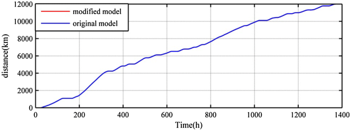
Distance
-
B.
Dynamic results
Apart from kinematic aspect, the dynamic factor is also considered in this braking system. Theoretically, the vehicle force achieved under the same driving conditions should be the same as that of simulation. As shown in Fig. 18, the experimental results of the modified model and the original model have the same vehicle power exactly. The results show the method can ensure braking safety of vehicle.
Fig. 18 
Vehicle force achieved
The wheel torque reflects the mechanical braking force exerted to the vehicle, as seen in Fig. 19. When wheel torque is positive, the vehicle is in a forward state; when the wheel torque is less than zero, the vehicle is in braking state. The modified model is coherent with the original one when the wheel torque is greater than zero, which means that the improved vehicle can reach the desired wheel torque under the driving forward condition. However, under the braking condition, the absolute wheel torque of the modified model is greater than that of the original wheel torque, which means that the wheels need to exert more torque. Therefore, more energy can be recovered during the braking process.
Fig. 19 
Wheel torque achieved
For the final drive torque outputs, gearbox torque outputs, and motor torque outputs, there are similar situations. According to Fig. 20, on the positive axis of y, the curve of the modified model overlaps completely with the original model curve; on the negative axis of the y, the absolute value of the modified model is much larger than that of the original. The simulation shows that, in the dynamic aspect, the driving safety can be ensured, and more torque will occur in the process of braking regeneration.
Fig. 20 
Final drive torque outputs achieved
To produce more energy, the motor should play a major role in the regenerative braking, and the gearbox torque output is another factor reflecting recirculation of the motor. As shown in Fig. 21, the improved model can recover more energy.
Fig. 21 
Gearbox torque outputs achieved
At last, the motor torque output figure gives the torque curve of motor during braking. In Fig. 22, the motor output torque is much larger during the braking process, so naturally more energy will be recovered in the process.
Fig. 22 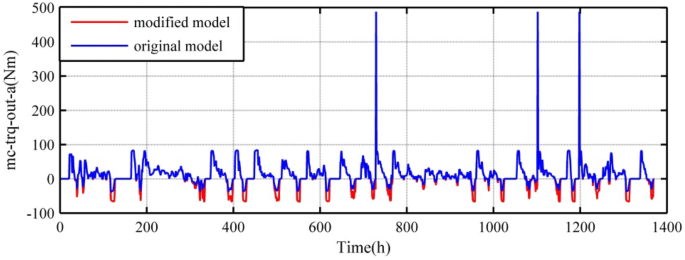
Motor torque outputs achieved


Energy Results
The energy storage history of SOC can be seen from Fig. 23. Obviously, the charging state in the modified model is higher than that of the original one by rough calculation, and the improvement value of SOC is about 15%. This is a convincing proof of the validity of the new control method in improving energy efficiency.

Energy storage history of SOC
As shown in Fig. 24, the modified model (red curve) can be found to be able to store more energy by comparing the energy in the storage system that varies with time.

Energy stored in the storage system varies with time
The above figures are all simulation results of the driving process, and the details of the energy recovery and usage of each part can be seen in Table 3.
According to Table 3, the energy efficiency of the modified control method is obviously better than the original one. In the modified model, both the input energy and output energy of motor/controller and gearbox have increased by (0.78 − 0.67)/0.67 = 16.42% and (0.94 − 0.9)/0.9 = 4.44%, respectively, which proves the effectiveness of the new control strategy. The energy consumed by brake is shown in the third column of Table 3. In the original model, the braking energy is 770 kJ, while, in the modified model, it is − 2630 kJ. Herein, the “ − ” means that the energy is increased in the modified model that is a direct proof of the validity of the modified control strategy. By calculation, the 3400 kJ energy can be recovered during regenerative braking.
Besides, in ADVISOR’s simulation software, a parameter named overall energy efficiency is defined. In the original model, the overall energy efficiency is 0.341, while the modified model is 0.374. The increase in energy efficiency is (0.374 − 0.341)/0.341 = 9.68%.
Conclusion
A novel regenerative braking control method is proposed. First, the force distribution regulation among the front-mechanical, the rear-mechanical, and the RBFs is designed. The regulation cannot only ensure the driving safety of vehicle, but also recycling more energy during braking process. Besides, using the fuzzy controller, a regenerative braking control method is designed. The controller includes the driver’s braking requirement and the vehicle speed related to the braking safety also considers the factors such as the battery SOC and temperature, which are important to ensure the battery safety. Furthermore, an HIL simulation experiment set-up and the simulation model system are established to testify the validity of the proposed strategy. Through experimental results, the driving safety can be ensured from the aspects of kinematics and dynamics, and energy utilization has increased about 10%. Therefore, the proposed RBS is an effective method to ensure driving safety and improving energy utilization efficiency.
References
Suganya S, Raja SC, Venkatesh P (2017) Simultaneous coordination of distinct plug-in hybrid electric vehicle charging stations: a modified particle swarm optimization approach. Energy 138:92–102
Gao MZ, Cai GP (2018) Fault-tolerant control for wing flutter under actuator faults and time delay. J Vib Eng Technol 6(6):429–439
Wu J, Wang X, Li L, Qin CA, Du Y (2018) Hierarchical control strategy with battery aging consideration for hybrid electric vehicle regenerative braking control. Energy 145:301–312
Chandak GA, Bhole AA (2017) A review on regenerative braking in electric vehicle. In: 2017 IEEE innovations in power and advanced computing technologies, Vellore, India, April, 21–22
Lot R, Massaro M (2017) A Symbolic approach to the multibody modeling of road vehicles. Int J Appl Mech 9(5):1750068
Zhang YF, Cesbron J, Yin HP, Berengier M (2017) Experimental study of normal contact force between a rolling pneumatic tyre and a single asperity. Int J Appl Mech 9(06):1750081
Ehsani M (2013) Switched reluctance motor drives, switched reluctance motor drives, for propulsion and regenerative braking, regenerative, braking, in EV and HEV. Encyclopedia of sustainability science and technology. Springer, New York
Lian YF, Tian YT, Hu LL, Yin C (2013) A new braking force distribution strategy for electric vehicle based on regenerative braking strength continuity. J Cent South Univ 20(12):3481–3489
Goodarzi A, Behmadi M, Esmailzadeh E (2010) Optimized braking force distribution during a braking-in-turn maneuver for articulated vehicles. In: IEEE international conference on mechanical and electrical technology, Singapore, September, 10–12
Fujimoto H, Harada S (2015) Model-based range extension control system for electric vehicles with front and rear driving–braking force distributions. IEEE T Ind Electron 62(5):3245–3254
Zhang J, Li Y, Chen L, Ye Y (2014) New regenerative braking controls strategy for rear-driven electrified minivans. Energy Convers Manage 82:135–145
Zhai L, Sun T, Wang J (2016) Electronic stability control based on motor driving and braking torque distribution for a four in-wheel motor drive electric vehicle. IEEE T Veh Technol 65(6):4726–4739
Li B, Goodarzi A, Khajepour A (2015) An optimal torque distribution control strategy for four-independent wheel drive electric vehicles. Veh Syst Dyn 53(8):1172–1189
Cai L, Zhang X (2011) Study on the control strategy of hybrid electric vehicle regenerative braking. In: IEEE international conference on electronic and mechanical engineering and information technology, Harbin, China, August, 12–14
Osborn R (2017) Vehicle and method of controlling a vehicle, US9718355
Qiu C, Wang G, Meng M, Shen Y (2018) A novel control strategy of regenerative braking system for electric vehicles under safety critical driving situations. Energy 149:329–340
Gao YM, Ehsani M (2010) Design and control methodology of plug-in hybrid electric vehicles. IEEE T Ind Electron 57(2):633–640
Mutoh N (2012) Driving and braking torque distribution methods for front and rear wheel-independent drive-type electric vehicles on roads with low friction coefficient. IEEE T Ind Electron 59(10):3919–3933
Yeo H, Kim H (2002) Hardware-in-the-loop simulation of regenerative braking for a hybrid electric vehicle. Proc Inst Mech Eng Part D-J Automob Eng 216(11):855–864
Guo J, Wang J, Cao B (2009) Study on braking force distribution of electric vehicles. In: Power and energy engineering conference (APPEEC 2009), Wuhan, China, March, 28–30
Gao Y, Chen L, Ehsani M (1999) Investigation of the effectiveness of regenerative braking for EV and HEV. SAE Trans 108:3184–3190
Li P, Jin DF, Luo YG (2005) Regenerative braking control strategy for a mild HEV. Autom Eng 27(5):570–574
Zou GC, Luo YG, Bian MY (2005) Simulation and study on control strategy for brake energy recovery of parallel type of HEV. Automob Tech 36(7):14–18
Zhao L, Tang L (2013) Braking force distribution research in electric vehicle regenerative braking strategy. In: IEEE international symposium on computational intelligence & design, Jia Zhou Hotel, Leshan, December, 14–15
Zhang XD, Göhlich D, Li J (2018) Energy-efficient toque allocation design of traction and regenerative braking for distributed drive electric vehicles. IEEE T Veh Technol 99(10):1
Gao Y, Ehsani (2001) Electronic braking system of EV and HEV—integration of regenerative braking, automatic braking force control and ABS. In: Future transportation technology conference and exposition, Ypsilanti, MI, June, 13–16
Oshima T, Fujiki N, Nakao S (2011) Development of an electrically driven intelligent brake system. SAE Int J Passeng Cars Mech Syst 4(6):399–405
Peng J, He H, Xiong R (2016) Rule based energy management strategy for a series–parallel plug-in hybrid electric bus optimized by dynamic programming. Appl Energy 185:1633–1643
Li L, Li X, Wang X, Song J, He K, Li C (2016) Analysis of downshift’s improvement to energy efficiency of an electric vehicle during regenerative braking. Appl Energy 176(8):125–137
Gao HW, Gao YM, Ehsani M (2001) A neural network based SRM drive control strategy for regenerative braking in EV and HEV. In: Electric machines and drives conference, (IEMDC 2001), Cambridge, MA, USA, June, 17–20
Yao J, Zhong ZM, Sun ZC (2006) A fuzzy logic based regenerative braking regulation for a fuel cell bus. Veh Electron Saf 12(8):22–25
Zhang JM, Song BY, Niu XJ (2008) Optimization of parallel regenerative braking control strategy. In: Vehicle power and propulsion conference, 2008 (VPPC ‘08) Harbin, China, September, 3–5
Li XJ, Xu LF, Hua JF, Li JQ, Ouyang MG (2008) Regenerative braking control strategy for fuel cell hybrid vehicle using fuzzy logic. Electric Mach Syst 10(5):2712–2716
Paul D, Velenis E, Cao D (2016) Tire-road-friction-estimation-based braking force distribution for AWD electrified vehicles with a single electric machine. In: IEEE international conference on sustainable energy engineering and application, Jakarta, Indonesia, October 03–05
Nian X, Peng F, Zhang H (2014) Regenerative braking system of electric vehicle driven by brushless DC motor. IEEE Trans Ind Electron 61(2):5798–5808
Guo JG, Dong HX, Sheng WH, Tu X (2018) Optimal control strategy for regenerative braking energy recovery of electric vehicle. J Jiangsu Univ (NATURAL SCIENCE EDITION) 39(17):132–138
ECE 13 (2005) Uniform Provisions Concerning the Approval of Vehicles of categories M, N and O with regard to braking. United Nations, Standards United Nations, New York
Yu ZS (2009) Automobile theories. China Machine Press, Beijing
Xu G Q, Li WM, Zheng L(2010) Regenerative braking for electric vehicle based on fuzzy logic control strategy. In: The 2010 international conference on mechanical and electronics engineering (ICMEE 2010), Kyoto, Japan, August, 25–27
Bouaziz H, Peyret N, Abbes MS, Chevallier G, Haddar M (2016) Vibration reduction of an assembly by control of the tightening load. Int J Appl Mech 8:1650081
Acknowledgements
The authors would like to acknowledge the financial supports from the NSFC (Natural Science Foundation of China, nos. 51705241, 11802118) and the NSFJP (National Science Foundation of Jiangsu Province, no. BK20170808).
Author information
Authors and Affiliations
Corresponding author
Additional information
Publisher's Note
Springer Nature remains neutral with regard to jurisdictional claims in published maps and institutional affiliations.
Rights and permissions
About this article

Cite this article
Zhang, Z., Dong, Y. & Han, Y. Dynamic and Control of Electric Vehicle in Regenerative Braking for Driving Safety and Energy Conservation. J. Vib. Eng. Technol. 8, 179–197 (2020). https://doi.org/10.1007/s42417-019-00098-0
Received:
Revised:
Accepted:
Published:
Issue Date:
DOI: https://doi.org/10.1007/s42417-019-00098-0