
Abstract
Musical instruments identification in polyphonic is a challenge in music information retrieval. In proposed work, a deep convolution neural network framework for predominant instrument recognition in real-world polyphonic music is accomplished. The network is trained on fixed-length music with a labeled predominant instrument and estimate an arbitrary number of instruments from an audio signal with variable length. The Mel spectrogram representation is used to map audio data into the matrix format. This work used eight layer convolution neural network for instrument recognition. ReLu activation function is used for the scaling of training data and introduces non-linearity in the network. At each layer, Max Pooling function is used for the dimension reduction. For the regularization, dropout is used which prevent the output from getting overfitting. The Softmax function gives the probability of particular instruments. The research excellent result with 92.8% accuracy.
1 Introduction
Artificial Intelligence [1] (AI) is modern technology which emphasizes creating a system which reacts like a human. It is an emerging field in the computer science. Nowadays many research like music generation, recommendation system, classification etc. takes place in the field of AI. The evolution and development of various algorithm and technique in the neural network make of advancement in the field of Artificial Intelligence.
1.1 Artificial neural network
ANN [1] is a biologically inspired model which perform on the computer and implemented with the help of mathematical logic. It is used for clustering [2], classification [3], prediction etc. It is an improved version of logistic regression [4] which is suitable for large data set. The Artificial Neural Network contains three layers as shown in Fig. 1. The first layer is called input layer which is responsible for taking input from the dataset in the form of a matrix, the second is called hidden layer which holds the weights, these weights get adjusted with the backpropagation algorithm [5] to get fit with the training dataset. In the third layer, the output is generated in the form of probability. There are different type of architecture in an artificial neural network such as recurrent neural network, Convolution neural network, capsule network etc. has revolutionizing AI industry.

Artificial neural network
1.2 Convolution neural network (CNN)
CNN [6] is class of ANN which is used generally in image classification, due to its convolution feature it identifies an object in any part of an image. It is a stack of Convolution Layer, Pooling Layer, and Fully-Connected Layer. It performs a series of operation on input data to derive the trend from it as shown in Fig. 2.

Convolution neural network
1.3 ALEXNET
In the proposed work ALEXNET [6] which is a modified version of CNN along with the functionality of CNN is used for analysis of spectrogram and recognition of music. It provides high accuracy with reduced computation time. The ALEXNET [6] uses dropout which provides regularization of the result and Leaky ReLu or ReLu activation function as described in Fig. 3. MaxPolling or Average pooling reduces the computation by reducing the arithmetic operation in the network.

AlexNet
2 Problem identification
It is uncomplicated for a human to identify the instruments that are used in a music, but for the computer, it is a difficult task to automatically recognize them. This is mainly because music in the real world is mostly polyphonic and extraction of information from audio become a tedious task. Furthermore, instrument sounds in the real world vary in many ways such as for timber, quality, and playing style, which makes identification of the musical instrument even harder. The musical sound has a large number of dimension which demands the high computational cost. For music instrument recognition there is the need for a high computational machine to process it and to produce the optimal result. The system gives revolution in the music industry by searching instrument according to the instrument.
3 Literature survey
In 2003 the handwritten digit recognition system using convolutional neural networks and Gabor filters was accomplished. A backpropagation algorithm specifically adapted to the problem is used in the training phase for the rest of the layers. Gabor filters as feature maps for the first layer of the network, instead of using a usual convolutional layer. Therefore, this modified network topology is called GCNN. The multiresolution analysis was used in order to obtain different feature maps for the first layer. A gradient-based algorithm, to adapt the weights of the other layers was used. Finally, it is shown that the use of committee machines improve the results [17]. In the year of 2004 musical instrument recognition on solo performances [15] was implemented using two statistical approach Gaussian Mixture Model (GMM) and the Support Vector Machines (SVM). The authors studied for the recognition of woodwind instruments using a large database of isolated notes and solo excerpts extracted from many different sources. The Principal Component Analysis (PCA) is used to de-noise. Mel-Frequency Cepstrum Coefficients (MFCC) as features, a study on isolated notes is discussed to test several variations on the classification strategies for model training and decision rules. In the year 2005 Instrument recognition in polyphonic music based on automatic taxonomies [18] is accomplished in which hierarchical clustering algorithm for exploiting robust probabilistic distances, authors obtain a taxonomy of musical ensembles which is used to efficiently classify possible combinations of instruments played simultaneously. A major focus of author work is Jazz music. In 2006 Classification of musical patterns using variable duration hidden Markov models [19] is accomplished which is the new extension to the variable duration Hidden Markov model (HMM), capable of classifying musical patterns that have been extracted from raw audio data into a set of predefined classes. Each musical pattern is converted into a sequence of music intervals by means of a fundamental frequency tracking procedure. This sequence is subsequently presented as input to a set of variable-duration HMMs. Each one of these models has been trained to recognize patterns of a corresponding predefined class. Classification is determined based on the highest recognition probability. In the year 2007 Pattern Recognition Approach for Music Style Identification Using Shallow Statistical Descriptors [20] is accomplished in which a framework covers the feature extraction, feature selection, and classification stages, in such a way that new features and new musical styles can be easily incorporated and tested. Different classification methods, like Bayesian classifier, nearest neighbors, and self-organizing maps, are applied in the study. In the year 2009 Music Scene- Adaptive Harmonic Dictionary for Unsupervised Note-Event Detection [21] is accomplished with the unsupervised process to obtain music scene-adaptive spectral patterns for each MIDI-note is proposed. Furthermore, the obtained harmonic dictionary is applied to note-event detection with matching pursuits. In the case of a music database that only consists of one-instrument signals, promising results (high accuracy and low error rate) have been achieved for note-event detection.
In the year 2010 a Survey of Audio-Based Music Classification and Annotation which highlights the new method and research area for Music information retrieval [22]. In the same year an Evaluation of Pooling Operations in Convolutional Architectures for Object Recognition [23] was proposed in which a comparison made on different aggregation function on the fixed architecture of several object recognition tasks. Empirical results show that a max pooling operation significantly outperforms subsampling operation.
In the year 2011 an automatic recognition of gesture using computer vision for many real-world application such as sign language and human–robot interaction [24] was accomplished using the state of the art big and deep convolution neural network with special max pooling MPCNN (Multi-Stage Hubel Wiesel Architecture). MPCNN is responsible for identifying the orientation of selective simple cells along with local receptive fields similar to those of convolution layers and complex cell performing sub-sampling like operation.
In the year 2012, the author proposed a system used for imagenet classification [6] with 1.2 million high-resolution images with 1000 different classes. To attain high computational performance max-pooling function used which decrease the computation by picking the max element from the sub input region and also a high amount of data cause overfitting problem to solve this dropout is used for regularization. In same year improving neural networks by preventing co- adaptation of feature detectors [7] was proposed in which a feed forward neural network is trained on small training set which not give good performance on test data. The overfitting is greatly reduced by omitting half of the feature detectors in each training case which prevent complex co-adaptation. Each neuron learns to detect a feature that is generally helpful for producing the correct results. Random dropout gives the improvement in many tasks of speech and object recognition. In 2014 Adam [16], an Adam algorithm for the first-order gradient-based optimization of stochastic objective functions, based on adaptive estimates of lower-order moments is used for optimization. The method is straightforward to implement, is computationally efficient, has little memory requirements, is invariant to a diagonal rescaling of the gradients, and is well suited for problems that are large in terms of data and/or parameters. The method is also appropriate for non- stationary objectives and problems with very noisy and/or sparse gradients. The hyper-parameters have intuitive interpretations and typically require little tuning. In the same year dropout [8] introduced in deep neural nets with a large number of parameters are very powerful but a large number also slow down the learning process dropout technique addresses this problem with dropout during training the some of the neuron output randomly restricted from generating weight.
In 2015 speech acoustic modeling from raw multichannel waveform [9] was proposed using CNN and DNN for the identification multichannel signal. In which timing between the input channels can be used to localize a signal in space. The system is trained on a signal channel with the long mel filter bank. It is trained on multichannel inputs. The network learns a filter-bank with a similar frequency scale that also exhibits directional selectivity to filter out energy coming from different spatial directions. It is essentially a bank of bandpass beam formers. Along with that Noisy image magnification with total variation regularization and order-changed dictionary learning [11] was accomplished in which provide two-step image magnification algorithm to solve Noisy image magnification problem. In the first step, total variation regularization takes place which is responsible for magnifying the LR image and at the same time suppressing the noise in it. In the second step with the ordered changed dictionary training algorithm to train dictionaries. Also in the same year, the investigation on the performance of the different type of rectified activation function in convolution takes place [10] which include ReLU, leaky ReLU, parametric ReLu and new Randomize leaky ReLU on standard images for classification. After evaluation it was found that non zero slope for a negative part in rectified activation unit gets improve consistently. In the same year Quang Trung Nguyen et al. proposed an approach for speech classification using SIFT [12] feature with Local Naive Bias Nearest Neighbour which allows using variable size feature vector. SIFT algorithm is designed to detect novel feature in images. The model uses the difference of Gaussian function as a kind of an improvement of gauss Laplace algorithm to achieve scale invariance.
In 2016 Deep Convolutional Neural Networks for Predominant Instrument Recognition in Polyphonic Music [14] is accomplished. In this work a convolution neural network is used for the predominant instrument Recognition is used. The model is trained on the singled labeled predominant instrument. The Max pooling is used for the dimension reduction of the network and Leky ReLU for the scaling. In the same year Speech dereverberation for enhancement and recognition using dynamic features constrained deep neural networks and feature adaptation [13] is accomplished. During training, a clean and distorted signal is used to map reverberant and noisy speech coefficients to underlying clean speech coefficients. The im- posed constraint by dynamic feature enhance the smoothness of predicted coefficient trajectories with least square estimation from predicted coefficient and other is incorporate the constraint of the dynamic feature directly into DNN.
In the year 2017 Head pose estimation in the wild using Convolutional Neural Networks and adaptive gradient methods [14] accomplished in which the performance of four architecture compared with recently released in the wild datasets. The result after combining CNN and adaptive gradient methods leads to the state of the art in unconstrained head pose estimation.
4 Musical instrument classification system using deep convolution neural network
This section discusses the architecture, process flow and pseudocode of the proposed system.
4.1 Architecture of proposed work
The proposed architecture as shown in Fig. 4. has mainly two module named training and a testing module which is discussed in this section.

Architecture of proposed work
4.1.1 I Training module
-
1.
Re-sampling training audio Signal: During the training phase, it is necessary to resample the audio near the Nyquist frequency to get the standard format of each input audio signal. The sampling frequency of 2200 is used in the proposed system.
-
2.
Audio window: The nonoverlapping window is used for dividing an audio signal into the frame. It should make sure that the frame is short enough so that it gets the reliable spectral estimate and long enough to observe the signal change.
-
3.
Mel Spectogram: Mel Spectogram [25] is a graphical representation of sound by using Mel scale on short time Fourier transformation generated the audio signal. The Network layer is the core of the proposed system responsible for the weight adjustment and fitting of training data. Initially, 3 × 3 convolution layer with 32 filters and Max Pooling function is used for the dimension reduction. For regularization and the prevention of over-fitting dropouts is used. The dropout eliminates some output from the predecessor layer to introduce desirable error in operation and prevent the result from over-fitting. The relu activation function is used in the proposed work for introducing non-linearity.
-
4.
Dropout: The dropout layer is responsible for regular- ization of output to prevent the result from over-fitting by introducing bias in a network.
-
5.
ReLu activation: ReLu activation function is responsible for introducing non-linearity in the network. ReLu reduces the computation and increases the accuracy of the result.
-
6.
Final weight: In the final step of the training phase, the final weight of each layer’s generated which then used for fitting and classifying testing data.
4.1.2 II Testing module
-
7.
Testing audio signal process: During the testing phase, the audio signal is sampled at the sampling rate of 2200 and the processed signal plotted using Mel-spectrogram.
-
8.
Prediction and classification with trained weight: This phase responsible for fitting testing signal to trained weight and classifying the instrument it gives result in posterior probability.
4.2 Process flow of proposed work
The process flow proposed work is describe in Fig. 5.

Process flow of proposed work step I input audio signal
Step I Input Audio Signal
The training data which is used in the proposed work is IMRAS dataset which contain the Western music recording. The IMRAS dataset consist 3 s audio clip of various music instrument. The training audio data re-sample at the sampling rate of 2200 and further re-sample audio signals normalized with short time Fourier transformation.
Step II Mel-Spectogram
Mel scale uses to compute the mel-spectrogram. The Mel Spectrogram represents the time–frequency representation of the audio signal. Mel Spectogram uses Mel filter and Mel Frequency to plot the signal. The Mel Filter is responsible for taking only those signal into consideration which falls under the range of Mel scale. Mel Filters function similar to human ears and the frequency at that range Mel scale is considered as Mel Frequency.
Step III Deep neural network
This step is a composition of feature reduction and classification. The Convolution Neural Network is responsible for the network layer operation. The convolution neural network generally uses in the classification of the image but in the proposed system. The audio signal behave as the image. On transforming audio signal into Mel-spectrogram.
III.A Max poolsing
The max pooling is used to down sample the dimension of the matrix and reduce the processing time. In proposed work 3 × 3 max-pooling layers are used which take most dominant value from submatrix with the nonoverlapping region.
III.B Dropout
The dropout provides the regularization to the result. The main function of dropout is to introduce a desirable error in the result the drop out rate used in the proposed work is 0.25.
III.C Activation function
The activation function that used in the proposed work is ReLu. The ReLu is more advance activation function than traditional activation function. The traditional activation function threshold the value to zero so it cause data input data to vanishing gradient problem but in ReLu the vanishing gradient is reduced.
III.D Optimizer
The Adam optimizer is used for calculating the error. It increases the network accuracy by maintaining the learning rate per parameter in the network and efficient result. Because of using a sparse gradient.
Step IV Result
The softmax function is used for calculating the posterior probability. The categorical cross entropy [26] calculate the normalized result of softmax function.
4.3 Pseudocode of proposed system
The proposed system functionality divided into two major parts training and testing.
-
1.
Pseudocode for training audio signal:

-
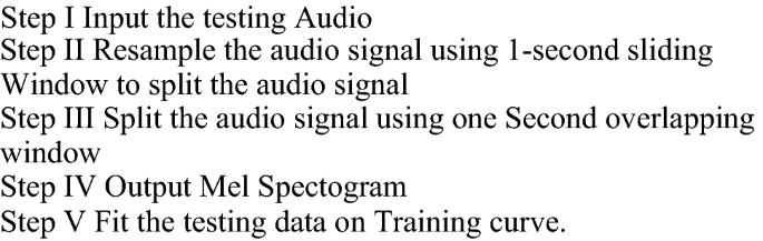
2.
Pseudocode for testing audio signal: Step I Input the testing Audio.


4.3.1 Implementation of proposed system
Python language is used to implement the proposed work on Ubuntu 16.04 with keras library and Tensorflow at the back end. The keras provide a high level of abstraction to the code with it ready-made model. The tensorflow at the back-end increase the system performance due to its operation at the GPU level. The Intel 2 GB graphic card used in this work with processor cycle of 2.65 GHz and 8 GB DDR 3 RAM on this configuration the training time take 985 min. The following step is used to implement the proposed system.
The dataset which is used in proposed work is from IMRAS dataset which is in the work of J. J. Bosch et al. for comparison of sound segregation techniques for predominant instrument recognition in musical audio signals [27]. It consists of audio of 11 musical instruments. The training data contain 6705 audio data for training as shown in Fig. 6.

IMRAS training data
Step I: Input Audio.
These data need to re sample in standard format. Sampling rate of 2200 to is used re sample the data. Figure 7 explains the waveform of the audio signal after resampling at the sampling rate of 2200.

Sampled audio signal
Step II: Audio signal processing.
To extract the features from audio spectrograms is used as shown in Fig. 8. Spectrograms have high dimension to decrease the dimensions with Mel spectrograms. The intensity of color defines the power of the audio signal at the different time of scale. Spectrograms have a set of color scheme which defines the volume/power of the audio signal. Spectogram is best for analyzing timber which is tune. The red region signifies the wave at the particular frequency scale and the intensity of the image signifies the power of a signal.

Spectogram of audio signal
Step III: Convolution layer.
In the convolution layer, the ALAXNET is used. It is a modified version of Convolution neural network. The two-dimension neural network with varying filter. The ReLu activation function introduces non-linearity in the result.
Step IV: Max polling.
The max pooling function is used to reduce the dimension of the result which results in an increase in computational and performance. The max pooling is described in Fig. 9. In the 3 × 3 max pooling it takes only max value from 3 × 3 submatrix into consideration.

Max pooling
Step V: Regularization.
For regulation dropout of 0.25 is introduced into the network which adds a bias in the network prevents the result from getting overfitting. Figure 10 describes the dropout functionality in which input to the next layer is accepted by blocking the output of some random nodes. Only 3 out of 4 output get computed in the next hidden layer which causes bias of one hidden layer output.

Dropout
Step VI: Second Layer of Network Layer.
In the second layer of network used 64 filters with the Max pooling of 3 × 3 and drop out of 0.25.
Step VII: Third Layer of Network Layer.
In the third layer of network used 128 filters with the Max pooling of 3 × 3 and drop out of 0.25.
Step VIII: Fourth Layer of Network Layer.
In the fourth layer of network used 256 filters with the Max pooling of 3 × 3 and drop out of 0.25.
Step IX: Fatten and Fully Connected Layer.
This layer responsible for getting input from all the layer combining them for the classification. The dropout of 0.5 layers is introduced in this layer.
Step X: Result.
The generated output is in the form of posterior probability. The categorical cross entropy is used to minimize the loss and Softmax function to calculate the posterior probability of each musical instrument. The network takes 60 epochs to set the weight with 92% accuracy.
5 Result
The proposed work is evaluated using the different parameter. At training, IMRAS dataset is used which contain 6705 western musical recording data. During the testing phase, 20% of the training data is used in a cross-validation set. The learning rate of 0.01 is fixed during the training with 9 layers deep neural network. Figure 11 shows the posterior Probability of the different instrument and the highlighted probability give the max probability of a particular instrument.

Output in the form of posterior probability
During the training it was observed that with each epoches, the accuracy increases. Figure 12 explain the training epoches vs accuracy curve with ReLu activation function and Max Pooling function.

Accuracy v/s epoches plot
The line graph shows negative movement in some points such as epoch 55 and epoch 56 at these point accuracy of the system is dropping because of overfitting.
-
1.
Max pooling and average pooling The Max Pooling picks up the most dominant feature from the sub-matrix of the input matrix and Average Pooling picks an average of the submatrix. An attempt is to used run an experiment with Average Pooling function for comparison with Max-Pooling function both with relu as an activation function. The bar graph in Fig. 13 compares the accuracy of Max Pooling and Average Pooling function.
Fig. 13 
Accuracy comparison of max pooling and average pooling
After analysis bar chart in Fig. 13, it is clear that there is the difference in result between two approaches and the Max Pooling gives the better outcome.
-
2.
ReLu Activation and Leaky ReLu activation function The ReLu activation function is responsible for introducing nonregularity and it appears to the most efficient and optimized activation function. An attempt is made to compare the accuracy of the system with LekyReLu which more advance then ReLu activation function by solving the vanishing gradient problem. Figure 14 gives the give the comparison result of both the activation function.
Fig. 14 
Accuracy comparison of ReLu and Leky ReLu


On comparing with different pooling operation and activation function. It is found that a combination of ReLu and Max Pooling function works best in proposed work. Figure 15 Give the comparison of results with different functions. Table 1 give the accuracy and Loss of system with a function of different parameter. From the table we can say that the Minimum loss and and highest accuracy is in combination of ReLu and max pooling function.

Accuracy comparison
5.1 Comparison with existing work
On comparison with the most recent work an improve in the accuracy by 4% is calculated. The recent work [14] uses deep convolution neural network with Leaky ReLu activation function and global Max Pooling at the end the final layer. An accuracy of 88% on cross-validation data sets is obtain. It was found that on using Max Pooling at the end of network instead of global Max Pooling the accuracy on cross-validation is increases and using ReLU activation function by increases accuracy by 4%.
During the testing, a confusion matrix obtained which get improved on introducing these changes. As discussed in Figs. 16 and 17. The confusion matrix of single music instrument gets improved by the significant level.

Confusion matrix of music instrument recognition using deep CNN [14]

Confusion matrix of proposed work
6 Conclusion
In the proposed work music instrument recognition using deep convolution neural network is accomplished. The system receives input in the form sampled audio signal which further converted Mel spectrogram form. The network receives input in the matrix representation form of Mel spectrogram. This work is accomplished using eight layers deep convolution neural network. The eight-layer provide the fitting of large datasets. It was found that ReLu activation function performs better in proposed work. Max Pooling function is used for dimension reduction. The dropout is used for preventing the result from overfitting. In the final layer, softmax function is used which calculate the probability of each musical instrument used in the audio signal. On comparing by with different function change it is found that the combination of ReLu activation function and Max Pooling is giving the best result in this work. After the 60 epochs, the research found the excellent result with 92.80% accuracy.
References
Purohit R et al (2013) AI and its application: sixth sense technology. Int J Emerg Trends Technol Comput Sci 2(3):184–186
Luong DTA, Chandola V (2017) A K-means approach to clustering disease progressions. 2017 IEEE International Conference on Healthcare Informatics (ICHI). https://doi.org/10.1109/ICHI.2017.18
Rong F (2016) Audio classification method based on machine learning. In: 2016 International conference on intelligent transportation. Big Data Smart City (ICITBS). https://doi.org/10.1109/ICITBS.2016.98
Issa MB et al (2017) Using logistic regression to improve virtual machines management in cloud computing systems. In: 2017 IEEE 14th international conference on mobile ad hoc and sensor systems (MASS). https://doi.org/10.1109/MASS.2017.86
Nitta T (1996) A back-propagation algorithm for complex numbered neural networks. In: Proceedings of 1993 international conference on neural networks (IJCNN-93-Nagoya, Japan). https://doi.org/10.1109/IJCNN.1993.716968
Krizhevsky A et al (2012) ImageNet classification with deep convolutional neural networks. In: NIPS’12 proceedings of the 25th international conference on neural information processing systems, vol 1, pp 1097–1105
Hinton GE (2012) Improving neural networks by preventing co-adaptation of feature detectors. Neural Evol Comput 1–18. arXiv:1207.0580
Srivastava N et al (2014) Dropout: a simple way to prevent neural networks from overfitting. J Mach Learn Res 15:1929–1958
Hoshen Y et al (2015) Speech acoustic modeling from raw multichannel waveforms. In: IEEE international conference on acoustics, speech and signal processing (ICASSP). https://doi.org/10.1109/icassp.2015.7178847
Xu B, Wang N, Chen T, Li M (2015) Empirical evaluation of rectified activations in convolutional network. CoRR. arXiv:1505.00853
Xu J, Chang Z, Fan J et al (2015) EURASIP J Adv Signal Process 2015:41. https://doi.org/10.1186/s13634-015-0225-y
Nguyen QT, Bui TD (2016) Vietnam J Comput Sci 3:247. https://doi.org/10.1007/s40595-016-0071-3
Xiao X (2016) Speech dereverberation for enhancement and recognition using dynamic features constrained deep neural networks and feature adaptation. EURASIP J Adv Signal Process 1:4
Han Y et al (2017) Deep convolutional neural networks for pre-dominant instrument recognition in polyphonic music. IEEE/ACM Trans Audio Speech Lang Process 25(1):208–221. https://doi.org/10.1109/taslp.2016.2632307
Slim ESSID et al (2004) Musical instrument recognition on solo performances. In: 2004 12th European signal processing conference, pp 1284–1286
Kingma DP, Ba J (2015) Adam: a method for stochastic optimization. CoRR. arXiv:1412.6980
Calderon A, et al. (2003) Handwritten digit recognition using convolutional neural networks and gabor filters. In: Proceedings of the international congress on computational intelligence CIIC, pp 1–9
Essid S et al (2006) Instrument recognition in polyphonic music based on automatic taxonomies. IEEE Trans Audio Speech Lang Process 14:1
Pikrakis A, et al. (2004) Classification of musical patterns using variable duration hidden Markov models. In: 2004 12th European signal processing conference
de Leon PJP, Inesta JM (2007) Pattern recognition approach for music style identification using shallow statistical descriptors. IEEE Trans Syst Man Cybern Part C Appl Rev 37(2):248–257
Carabias-Orti JJ et al (2010) Music scene-adaptive harmonic dictionary for unsupervised note-event detection. IEEE Trans Audio Speech Lang Process 18(3):473–486
Fu Z et al (2011) A survey of audio-based music classification and annotation. IEEE Trans Multimedia 13(2):303–319. https://doi.org/10.1109/TMM.2010.2098858
Scherer D, Mller A, Behnke S (2010) Evaluation of pooling operations in convolutional architectures for object recognition. In: Diamantaras K, Duch W, Iliadis LS (eds) Artificial neural networks ICANN 2010. ICANN 2010. Lecture Notes in Computer Science, vol 6354. Springer, Berlin
Nagi J (2011) Max pooling convolution neural networks for vision- based hand gesture recognition. In: 2011 IEEE International Conference on Signal and Image Processing Applications (ICSIPA)
Weenink D (2016) Speech signal processing with Praat 18th April 2016
Plunkett K, Elman JL (1997) Exercises in rethinking innateness. MIT Press, Cambridge, p 166
Bosch J, et al. (2012) A comparison of sound segregation techniques for predominant instrument recognition in musical audio signals, 13th International society for music information retrieval conference (ISMIR 2012) pp. 559–564
Author information
Authors and Affiliations
Corresponding author
Rights and permissions
About this article

Cite this article
Solanki, A., Pandey, S. Music instrument recognition using deep convolutional neural networks. Int. j. inf. tecnol. 14, 1659–1668 (2022). https://doi.org/10.1007/s41870-019-00285-y
Received:
Accepted:
Published:
Issue Date:
DOI: https://doi.org/10.1007/s41870-019-00285-y