Design of Path Planning and Obstacle Avoidance for a Wheeled Mobile Robot

Abstract

This paper proposed a path tracking method for wheeled mobile robot (WMR). This method includes path planning and controller design. In path planning, using B-spline instead of A* algorithm to create smooth and obstacle-avoidance path, so that the possibility of collision can be reduced statistically. In controller design, genetic algorithm (GA) and fuzzy logic control (FLC) are combined together for the velocity control for WMR, which is supposed to move in a certain environment. The suitable membership function of FLC according to the feature of environment, such as distance and angle of WMR, is based on the B-spline path, and the input and output of FLC can be adjusted by GA. Therefore, the WMR can move along the planned path steady, which means our method has good performance.

1 Introduction

Recently, robots are paid more and more attention by many people [1–3]. According to the structure of mobile robot, we can classify into foot robots and wheeled robots. The former, with complex mechanism design problem, should be considered balancing themselves during working. Literatures [4–6] have discussed these issues. Conversely, the latter are simplified as mechanism, we only have to know each part of robot’s size, such as platform, wheels, and sensors, then deriving mathematical model from their structure and consider how to control them [7–9].

In past research, one of the most important task of WMR is path planning, which is to navigate the robot to the destination quickly and safely. In order to satisfy these demands, especially for obstacle avoidance [10], the location of robot is an indispensable information for path planning. If the robot moves in the unknown surrounding, the technology, such as simultaneous localization and mapping, can be used helpfully with the information from camera or ulreasonic range sensor. However, this paper focuses only on the known surrounding to reduce the complexity of system.

In order to achieve the shortest path and the lowest time cost, we adopt A* algorithm to find the shortest path [11]. Comparing with the well-known Dijkstra's algorithm [12], the latter can also be guaranteed to find the shortest path, but its performance is not as fast as the former. When Dijkstra's algorithm does not likely seem to be applied to some situations considering time cost, the improved algorithm of Dijkstra, A* algorithm, is regarded as the more suitable method in this paper.

The idea of B-spline curve was proposed by Schoenberg in 1946 [13]. Others like Bezier curve [14] or Cubic curve [15] are used to design obstacle-avoidance paths for robots. However, B-spline curve is more widely used than the others for its ability of local controlling, adding control points of curves without changing their orders, and bringing up different order curves when fixing B-spline’s control point on the other hand.

Genetic algorithm, one of the evolutionary algorithms, is a search heuristic algorithm [16] to solve optimization in the artificial intelligence field of computer science. This heuristic is usually used to generate useful solutions for optimization and searching problems. Evolutionary algorithm is originally developed by some phenomena among evolutionary biology, these phenomena include genetic, mutation, natural selection and hybridization.

Genetic algorithm really has been widely used among bioinformatics [17], phylogenetic, computer science [18], engineering, economics, chemistry, manufacturing, mathematics, physics, science, and other areas of drug measurement, such as C wing, air plane, water supply, games, TSP, learning scenes, coding A face, freeze/flood, simulation crime, etc.

Controlling is a new and evolving subject; there were some names such as expert control [3], learning control, and others have been mentioned beforehand. Intelligent control has been more able to be accepted recently, such as fuzzy logic control (FLC) which is a thinking pattern applied using human reasoning to decide how to control models, that is imitating the way people think of fuzzy phenomenon or things, by way of experts’ judgment and then make decision to solve complex control problems. Genetic algorithm is based on the theory of evolution, belonging to wise method [19]. Wisdom control is an effective way of system’s control, but this does not mean that the traditional control is no wisdom, we may better say that intelligent control uses human intelligence to handle affairs, and make some decisions. On the contrary, traditional control way uses mathematical derivation out of control, and it’s less thinking action in the control process.

In modern control, three feature objects are often encountered and they are given in the following:

• Uncertainty Model of the controlled substance not available or uncertain, unsure of model parameters.

• Nonlinear Nonlinear increasingly complex-controlled body presented, even nonlinear control theory, also not perfect, it would not be able to solve all the nonlinear problems.

• Complex Objectives For example, robust control not only considered performance, but considered robust features about foreign interference and internal system’s parameters. Mission requirements are becoming increasingly complex, as a result, only using traditional control will not be applied.

GA is a kind of evolutionary algorithms that can deal with optimization problem. Fuzzy controller is a language controller that allows the operator to easily use natural language to access man–machine dialogue, and do not have to establish a complete mathematical model of the controlled object. In the past, many experts have been able to combine the two ways of dealing with the path planning and obstacle-avoidance problems in WMR [3, 20].

All of the above applications are to solve the mathematical maximization or minimization questions. If function is differentiable, it can be optimized by gradient methods; if not, there are other ways, such as simulation annealing, random search method, etc. There is a common feature among these methods, the results found may be global optimum or local optimum. And the best advantage of genetic algorithm is avoiding falling into local optimum point during the optimization process of seeking, so the chances to find the best global point would be great. This is mainly accredited to the ability of induced mutations. Even if genetic algorithm may not find the best answer every time, the result always appears near the best answer, unlike the other methods with big opportunity that have their answers fall on the second best point.

This paper is organized as follows. In Sect. 2, we establish some mathematical model of WMR used for motion discussion and robotic control. In Sect. 3, description to the algorithms’ theorem about A* algorithm and B-spline curve used for path planning is given in this paper. In Sect. 4, the part concept of GA which is used in this paper is selected and described. In Sect. 5, description to the theorem of FLC and flow of control design is given. In Sect. 6, adoption to the simulation of path planning and path tracking way is given.

2 Kinematic of Wheeled Mobile Robot

Wheeled robot used in this study is composed of three rigid bodies, each of them are platform, fixed wheel installed on each sides of the platform.

The purpose of this part is to get the motion equations of the robot, so we need to analyze its structure, and then derive the geometric and kinematic constraints.

In Fig. 1, let body1 be platform, body2 and body3 are the wheels fixed to the robot left and right sides, and the freedom wheel is not be considered in the derivation process.

Fig. 1

Define body of WMR

In the following we define some parameters for robot: w _r is radius of the wheel, L is half distance between two wheels. In the three-dimensional space, each of the rigid body needs six variables to describe the relationship between movement and rotation, so in this study we use $x = \left( {x_{i} , y_{i} , z_{i} , \varphi_{i} , \delta_{i} , \theta_{i} } \right),i = 1, \, 2, \, 3,$ represents variables, (x _i , y _i , z _i ) is described as rigid body’s coordinates on the inertial coordinate axis, then $(\varphi_{i} ,\,\delta_{i} ,\,\theta_{i} )$ is described as attitude angle of rigid body, each of them represents the roll angle, the pitch angle, and the yaw angle, and i is the corresponding number of rigid mentioned beforehand.

Here define X-axis as the moving direction of robots, Z-axis as direction toward the earth, Y-axis is right-handed coordinate system from X-axis and Z-axis. Therefore, according to this definition we can get $(\varphi_{i} ,\,\delta_{i} ,\,\theta_{i} )$ as the three rotation angles of shaft on X-, Y-, Z-axis.

Because attitude angle is defined in the robot, it is relative with robot’s movement, and each wheel has common axis and is perpendicular to the moving direction, therefore the angular direction of the wheel and platform is consistent and then we get:

$$ \theta_{2} = \theta_{1} $$

(1)

$$ \theta_{3} = \theta_{1} $$

(2)

The position of rigid is affected by robot’s structural constraints, therefore there are these following constraints:

$$ x_{2} = x_{1} + d\cos \theta_{1} - L\sin \theta_{1} $$

(3)

$$ y_{2} = y_{1} + d\sin \theta_{1} + L\cos \theta_{1} $$

(4)

$$ x_{3} = x_{1} + d\cos \theta_{1} + L\sin \theta_{1} $$

(5)

$$ y_{3} = y_{1} + d\sin \theta_{1} + L\sin \theta_{1} $$

(6)

After the above six robot motion model geometric constraints, the next step includes motion restrictions and we derive it.

Considering wheels are pure rolling state on the ground, the moving speed is relative to the rotation angular velocity and the robot’s moving direction, as per the following four sports constraints:

$$ \dot{x}_{2} = r\dot{\delta }_{2} \cos \theta_{1} $$

(7)

$$ \dot{y}_{2} = r\dot{\delta }_{2} \sin \theta_{1} $$

(8)

$$ \dot{x}_{3} = r\dot{\delta }_{3} \cos \theta_{1} $$

(9)

$$ \dot{y}_{3} = r\dot{\delta }_{3} \sin \theta_{1} $$

(10)

By (3), (5), we can get:

$$ x_{3} - x_{2} = 2L\sin \theta_{1} $$

(11)

Differential form of (11) is the following:

$$ \dot{x}_{3} - \dot{x}_{2} = 2L\cos \theta_{1} \cdot \theta_{1} $$

(12)

Including motion constraints (7) and (9) we have the following:

$$ w_{\text{r}} \left( {\dot{\varphi }_{2} - \dot{\varphi }_{3} } \right)\, = \,2L\dot{\theta }_{1} $$

(13)

Since this equation can be integral, it can be converted into a geometric constraint:

$$ \theta_{1} = \frac{r}{2L}\left( {\delta_{3} - \delta_{2} } \right) + c_{2}, $$

(14)

where C ₂is a constant, θ ₁ represents initial value. In addition, from (3) to (6) also can be obtained:

$$ x_{2} + x_{3} = 2x_{1} + 2d\cos \theta_{1}, $$

(15)

$$ y_{2} + y_{3} = 2y_{1} + 2d\sin \theta_{1}, $$

(16)

respectively, and to the left after the equal sign and the differential was:

$$ \dot{x}_{1} = \frac{1}{2}\left( {\dot{x}_{2} + \dot{x}_{3} } \right) - d\cos \dot{\theta }_{1} \cdot \theta_{1} $$

(17)

$$ \dot{y}_{1} = \frac{1}{2}\left( {\dot{y}_{2} + \dot{y}_{3} } \right) + d\cos \dot{\theta }_{1} \cdot \theta_{1} $$

(18)

The motion constraints (7) to (10) after the substitution and they were analyzed to obtain:

$$ \dot{x}_{1} = \frac{{w_{\text{r}} }}{2}\left( {\dot{\varphi }_{2} + \dot{\varphi }_{3} } \right)\cos \theta_{1} - d\cos \dot{\theta }_{1} \cdot \theta_{1} $$

(19)

$$ \dot{y}_{1} = \frac{{w_{\text{r}} }}{2}\left( {\dot{\varphi }_{2} + \dot{\varphi }_{3} } \right)\sin \theta_{1} + d\cos \dot{\theta }_{1} \cdot \theta_{1} $$

(20)

Compared with the platform coordinates (x ₁, y ₁), the central reference point Pr(x _r, y _r) around the axle use it more often, and because the wheel is mounted on the servo motor, it can be controlled directly, in this order $\dot{\delta }_{2} \, = \,u_{1}$ and $\dot{\delta }_{3} \, = \,u_{2}$, and finally we can get sports model robots:

$$ \begin{aligned} \dot{\delta }_{2}&=u_{1} \hfill \\ \dot{\delta }_{3}&=u_{2} \hfill \\ \dot{x}_{\rm r} &= \frac{r}{2}\left( {u_{1} + u_{2} } \right)\cos \theta_{1} \hfill \\ \dot{y}_{\rm r} &= \frac{r}{2}\left( {u_{1} + u_{2} } \right)\sin \theta_{1} \hfill \\ \dot{\theta }_{1}& = \frac{r}{2L}\left( {u_{1} - u_{2} } \right) \hfill \\ \end{aligned} $$

(21)

3 Path Planning

3.1 A* Algorithm

A* algorithm determines the lowest path-limited nodes by least cost [21]; mathematic form is represented as (22). This algorithm contains two stages: search and reconstruction phase. When g(n) represents the actual distance from the start point n0 to any node n, and h(n) represents any node n to estimate the distance to the target point ng, the overall cost can be expressed as a function of the distance

$$ f({\mathbf{n}}) = g({\mathbf{n}}) + h({\mathbf{n}}) $$

(22)

When h(n) is less than the actual distance from the node n to the destination point, then you can certainly get the shortest path, and if h(n) is close to the practical cost, this algorithm will be the most efficient. But if h(n) is larger than the practical cost, the result will not be guaranteed. In the practical operation, we usually define h(n) to be the distance between current node and target point. Operation process of A* algorithm is as follows and the result is as shown in Fig. 2.

Fig. 2

Path planning by A* algorithm

Step 1 to Step 10 belong to searching stage, it’s to find the goal point with the lowest cost, and Step 11 to Step 13 belong to reconstruction stage, it’s to establish the result of path with all the nodes that had been found.

Step 1:

Establish OPEN array and CLOSE array. OPEN array sets forthcoming nodes that will be estimated, CLOSE array sets the nodes which was completed computing. OPEN array as the starting point n ₀; CLOSE array was empty. g(n) as the actual lowest cost from start point n ₀ to the node n, and it is possible to obtain g(n ₀) as zero. In this step while estimating h(n ₀), the result g(n ₀) = 0 to obtain f(n ₀) = h(n ₀).

Step 2:

Construct a loop from step 3 to step 10, if OPEN array is nonempty, then calculate into the loop, it means it still did not arrive to the end, and after judgment, if no path to the end is generated, then return fail plan.

Step 3:

From OPEN array find the node which has smallest f(n), and regard it as next current node x, determining whether it is the end point n _g, if so, it means that the search step is completed, then remove the target node from OPEN array and add to CLOSE array, out of step 2 and go to step 11.

Step 4:

Search in the vicinity from the current node and reachable nodes defined as y _i .

Step 5:

Construct a loop containing step 5 to step 10, judging each nodes y _i in the loop until all adjacent node judgment is completed.

Step 6:

Determine whether the nodes y _i are in the CLOSE array, skipping this node, determining the next adjacent nodes, or continue to the next step.

Step 7:

Evaluating g(y _i ) of y _i , this function is defined by the current actual cost function node x, and can be expressed as $\hat{g}(y_{i} )\, = \,g(x)\, + \,{\text{dis}}(x,y_{i} )$, which dis() function represents linear distance between nodes.

Step 8:

Setting a Boolean parameter k is false, recording whether the node information needs to be updated.

Step 9:

Determining whether nodes y _i are in OPEN array, if not, the node y _i will be added in OPEN array, and define whether parameter k is true, or it is again judged $\hat{g}(y_{i} )$ whether it is less than g(y _i ) at node y _i , if so, parameter k is then set true, to indicate that the node data need to be added or modified.

Step 10:

Analyzing the parameters k, if it is false, then go straight back to Step 5, if it is true then update the information, comprising: set node y _i source node as x, it is represented by the current node x and g(y _i ) substituted by $\hat{g}(y_{i} )$ indicating that there is a lower cost path.

Step 11:

This is the reconstruction stage, let the goal point n _g of the path temporarily store P first position, i.e., P(1) = ng.

Step 12:

Constructing of a loop, in accordance with P(i + 1) = c(P(i)), filling N nodes information gradually in the temporarily stored path, until the starting point is added to the temporarily stored path, which satisfies P(N) = n ₀.

Step 13:

Overturning the order in temporarily stored path, namely P(i) = P(N − i + 1), i = 1,2,…, N − 1, then will have the correct order path P, namely to complete the A* algorithm.

3.2 B-Spline Curve

Path planning is not usually able to accurately design a path to meet user’s demand by one type of algorithm; the results from the previous design way in Fig. 2 shows that there are too many corners during the path that are not continuous and not suitable for real mobile robots to track with their body size, in order to overcome such problems, having characteristics of local adjusting with B-Spline curve will look quite apply.

B-spline curve is generated by a set of base functions and parameters of control points, consisting of affine invariant, adjustments in the local curve, convex hull property, continuity and differentiability superior qualities, etc., making it more suitable as a smooth description method curve. B-spline curve’s mathematical model is represented as follows:

$$ P(t) = \sum\limits_{i = 0}^{n} {P_{i} N_{i,k} (u)}, $$

(23)

where P(t) is position vector on the curve along with parameter t, B _i is position vector control points, also named control points, the number of it is n + 1, N _i,k is normalized B-spline basis function. At the order k (degree k − 1), Cox-de Boor regression formula of i _th basis function N _i,k (t) is defined as follows:

$$ N_{i,1} (u) = \left\{ {\begin{array}{ll} 1 &\quad {{\text{if t}}_{{i}} \le u < t_{i + 1} } \\ 0 & \quad {\text{others}} \\ \end{array} } \right. $$

(24)

and

$$ N_{i,k} (u) = \frac{{(u - t_{i} )N_{i,k - 1} (t)}}{{t_{i + k - 1} - t_{i} }} + \frac{{(t_{i + k} - u)N_{i + 1,k - 1} (u)}}{{t_{i + k} - t_{i + 1} }} $$

(25)

defines 0/0 = 0 during calculating.

t _i is named as knot value, and {t _i } is named as knot value, and the knot value is defined as (26)

$$ \begin{array}{*{20}l} {t_{i} = 0,} &\quad {i = 0, \ldots ,k - 1} \\ {t_{i} = i - k + 1,} &\quad {i = k, \ldots ,n} \\ {t_{i} = n - k + 2, \, } &\quad {i = n + 1, \ldots ,n + k} \\ \end{array} $$

(26)

x _i is the ith element of node vector, and x _i  ≤ x _i+1, t is between t _min and t _max. In (25). For k = 3 as example, assuming k = 3, we then used (23)–(26) and then the basic function is given in Table 1 and the result is shown in Fig. 3.

Table 1 Basic function of k = 3

Fig. 3

B-spline curve(n = 4, k = 3)

k = 3 (order = 3), k not value: {0, 0, 0, 1, 2, 3, 3, 3} = {t ₀, t ₁, t ₂, t ₃, t ₄, t ₅, t ₆, t ₇} by the procedure and by defining the position of control point we can find the value P(t).

The curve of order k (degree k − 1) usually satisfies the following conditions:

• P(t) should be the polynomial degree k − 1 in any region of x _i .

• P(t) contains both differential and continuity of 1 to k − 2 order.

• In the valid region of t, N _i,k  ≥ 0, and each of N _i,k has only one maximum value, and N _i,k is the continuous smooth curve except k = 1, 2.

4 Genetic Algorithm

Genetic algorithm is usually implemented as a way of computer simulation [21]. It contains Gene, Chromosome, Fitness function, and Population for the elements for algorithm. For an optimization problem, a number of candidate solutions’ abstract representation of the population is to evolve to a better solution. Traditionally, the solution is usually represented with binary (strings 0 and 1), but also can use other representation [22]. Evolving begins from completely random individual populations, then occurred on next generations. In each generation, the fitness of the entire population is evaluated, choosing multiple individuals (based on their fitness) randomly from the current population, generating new life populations through natural selection, and the population in the last iteration of the algorithm becomes the current population.

The strategy of genetic algorithm is shown in Fig. 4, its procedure contains initially, evaluation, selection, crossover, mutation, and brings new chromosomes, next we focus on each procedure and discuss them in detail.

Fig. 4

Procedure of GA

• Encoding. In order to facilitate mating with crossover and mutation, genes should be encoded into binary digits and called as chromosome. Genetic algorithm which consisted of coded procedures is binary genetic algorithm, if genetic algorithm’s parameter is directly composed of floating, it is called real genetic algorithms, continuous parameter genetic algorithms, or floating point genetic algorithms (RGA, CGA, or FPGA). Generally, real number converts to binary number using direct binary conversion (straight binary), for example, if x is from 0 to 10, and represented by bit length number 7, then the decimal and binary number is represented as follows:

  0 → 000 0000 (=0)

  100 → 111 1111(=127)

  then 50 = fix(0.5*127) = 63 is selected, that is 0111 111. But the number 011 1111 represents 100 × (63/127) = 49.606 actually, rather than 50. Because there are 128 binary numbers, therefore a real number from 0 to 100 can only correspond to 128 bits, instead of infinite number. This is called Quantization. The greater the number of bit length to represent, the more it means more accurate (resolution). The disadvantage is that the longer transcoding time will slow down execution time of program. The conversion formula is

  $$ x\, = \,{\text{B}}2{\text{D}}\, \times \,\left( {{\text{UB}} - {\text{LB}}} \right)/\left( {2^{l} - 1} \right)\, + \,{\text{LB}}, $$

  (27)

  where B2D is transfer from binary to decimal, i.e., 1101 → 13, UB is maximum value, LB is minimum value, L is bit length, x is gene’s real value, for example, UB = 100, LB = 0, binary = 0111 1110, then B2D = 126, L = 8,

  $$ x = 126 \times (100 - 0)/(2^{8} - 1) + 0 = 49.412 $$

  Next, for calculating fitness function, we have to transfer binary after encoding procedure to decimal, called “Decoding.”

• Evaluation and Selection Here we introduce the way Roulette Wheel Selection. In Fig. 3, the proportion of the round can be thought as each selection’s probability represented in (28).

  $$ \left\{ {\begin{array}{ll} {f_{1} = 4} \\ {f_{2} = 3} \\ {f_{3} = 3} \\ {f_{4} = 2} \\ \end{array} } \right. \quad p_{i} = \frac{{f_{i} }}{{\sum\limits_{j} {f_{j} } }} $$

  (28)

  f _i is value of fitness function, here defined by number of ′1′ in binary as Figs. 5 and 6

  Fig. 5

  

  Value of fitness function

  Fig. 6

  

  Roulette wheel selection

• Crossover Select two sets of data for mating to match, then set new chromosome into the next generation of ethnic groups as in Fig. 7.

  Fig. 7

  

  Crossover in GA

• Mutation Mutation as shown in Fig. 8 is to produce new varieties so that searching for the best values will not be trapped in a local maximum or local minimum value.

  Fig. 8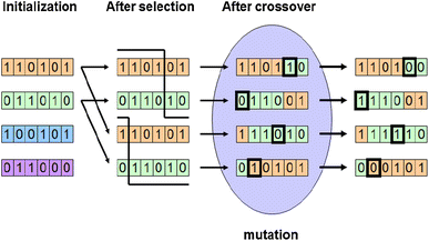

  

  Mutation in GA

The probability of mutation is signed as, it’s value usually provided between 0.01 and 0.08 generally, when set 0 may let genetic algorithms not get the best results, if too large, it can’t to be convergence. If there are 100 chromosomes, and P _m = 0.08, then the average of eight chromosome will be mutated (determined by the random number generated). General mutation is just select one bit during string randomly, original 0–1, and original 1 becomes zero.

5 Fuzzy Control Theorem

Fuzzy control is a way of using FLC to control plants. FLC is composed according to Fuzzy set theory advocated by Professor Zadeh’s in 1965 [23] and consists of an inference to generate control signals. You can design such a controller without a proper mathematical model of the controlled substance (differential equations or transfer functions to start the design). Fuzzy theory now contains fuzzy set, fuzzy logic, fuzzy measure, fuzzy inference system, fuzzy numbers, fuzzy integral, fuzzy entropy, etc.

Fuzzy inference logic does not require complicated mathematical operations (such as differential, integral, or floating point of error), maybe a rule table could complete the entire fuzzy controller inference result. On the other hand, the best benefit of fuzzy controller is saving the excessive computational load during performing table look-up process. It makes the system capable to execute control algorithms sufficiently in small sampling time, and ensures robots’ control quality and results of path tracking, Fig. 9 is the content of fuzzy control procedure, and the following describes each site of flow of fuzzy logical control.

Fig. 9

Procedure of Fuzzy control

• Fuzzification: It’s the step of conversion input data into equivalent language value, quantifying, and setting up membership function.

• Fuzzy rule: It’s causal relationship between input and output “IF, THEN” design rules, for example,

  $\begin{aligned} R^{1} :\,{\text{IF }}X_{1} {\text{ is }}A_{11} {\text{ AND }}X_{2} {\text{ is }}A_{21} {\text{ THEN }}Y{\text{ is }}B_{1} \hfill \\ {\text{R}}^{2} :\,{\text{IF }}X_{1} {\text{ is }}A_{12} {\text{ AND }}X_{2} {\text{ is }}A_{22} {\text{ THEN }}Y{\text{ is }}B_{2} \hfill \\ \end{aligned}$ then here we use the “max–min operation” to inference output as shown in Fig. 10.

  Fig. 10

  

  Max–min operation

• Inference Engine: It’s the step that lets fuzzy input set via fuzzy logic inference, combining with all IF–THEN rules then mapped to fuzzy output set via the fuzzy rule base.

• Defuzzification The process of converting conclusions generated by the fuzzy inference into explicit value. Here “centroid method” is provided in Fig. 10 as a way of defuzzification to solve overlap region of membership function, define fuzzy set C as conclusion of the fuzzy rules after fuzzy inference procedure, and y is the result of the solution after defuzzification. Following are the two formula forms in different situation.

When the range is continuous

$$ y^{*} = \frac{{\int_{Y} {\mu_{\text{C}} (y) \cdot y{\text{d}}y} }}{{\int_{Y} {\mu_{\text{C}} (y)\;{\text{d}}y} }} , $$

(29)

$\smallint$ represents symbol of continuous.

When the range of discrete time

$$ y^{*} = \frac{{\sum\nolimits_{i = 1}^{L} {\mu_{\text{C}} (y_{i} )} \cdot y_{i} }}{{\sum\nolimits_{i = 1}^{L} {\mu_{\text{C}} (y_{i} )} }} , $$

(30)

∑ represents symbol of discrete time. μ _c(y _i )is ith grade of membership about output’s rule set, and yi is output value of ith rule.

6 Simulation

In this section, we try to let the robot move along a path which had been designed, and when robot meets an obstacle, it also can avoid obstacle successfully. We planned the shortest path from start to destination of WMR by A* algorithm and let WMR move along it as shown in Fig. 11; the red line is the shortest path by A* algorithm. Because the real robots should have their specific size, when WMR meets obstacles, we deal with the procedure in avoidance of obstacle by the design of a new obstacle-avoidance path as shown in Fig. 12 [24]. Equation (31) is transfer from Cartesian coordinate to the new coordinate based on the direction of WMR.

Fig. 11

Path planning of shortest path with A* algorithm

Fig. 12

Tracking of avoidance path

$$ \left[ {\begin{array}{*{20}c} {\xi_{\text{e}} } \\ {\eta_{\text{e}} } \\ {\theta_{\text{e}} } \\ \end{array} } \right] = \left[ {\begin{array}{*{20}c} {\cos \theta } & {\sin \theta } & 0 \\ { - \sin \theta } & {\cos \theta } & 0 \\ 0 & 0 & 1 \\ \end{array} } \right]\left[ {\begin{array}{*{20}c} {x_{\text{d}} - x_{\text{r}} } \\ {y_{\text{d}} - y_{\text{r}} } \\ {\theta_{\text{d}} - \theta } \\ \end{array} } \right] $$

(31)

The error parameters between reference path and WMR’s direction are defined as (x _e, y _e, θ _e), and

$$ x_{\text{e}} \, = \,x_{\text{d}} \, - \,x_{\text{r}} ,\,y_{\text{e}} \, = \,y_{\text{d}} \, - \,y_{\text{r}} ,\,\theta_{\text{e}} \, = \,\theta_{\text{d}} \, - \,\theta_{\text{r}} $$

are also defined as $d_{\text{e}} \, = \,\sqrt {\xi_{\text{e}}^{2} + \eta_{\text{e}}^{2} } ,\,\vartheta_{\text{e}} \, = \,\tan^{ - 1} (\eta_{\text{e}} /\xi_{\text{e}} )$, d _e is distance between WMR’s current position and goal on the avoidance path, ϑ _e is line of sight angle from WMR’s direction to goal.

After some parameters have been defined, we then use d _e, θ _e, ϑ _e as input of FLC, and Δs ₁, Δs ₂ as output, each Δs ₁, Δs ₂ is represented as linear and angular velocity of left wheel, respectively. Each of the Figs. 13 and 14 represent the membership function of fuzzy input and fuzzy output. Table 2 shows the suitable fuzzy rule to achieve the proposal of path tracking on new avoidance path planned by B-spline curve, it’s considered by some situation:

Fig. 13

Membership function of fuzzy input parameter. a d _e, b θ _e, c $\vartheta_{\text{e}}$

Fig. 14

Membership function of fuzzy output parameter

Table 2 Fuzzy rule of path tracking

S1:

When ϑ _e is close to zero and θ _e is small, it should move fast forward and avoid any turning action, design angular velocity Δs ₂ → 0.

S2:

When d _e → 0, it’s much important to adjust Δs ₂ than Δs ₁. Here Δs ₁ → 0 is defined and Δs ₂ is changed with θ _e.

S3:

When d _e is too large, robot will only move in forward motion without rotating (Δs ₂ → 0).

S4:

Δs ₂ decreases when d _e increases and keeps increasing when $\left| {\vartheta_{\text{e}} } \right|$ and $\left| {\theta_{\text{e}} } \right|$ increase.

S5:

Δs ₁ increases when d _e increases and keeps decreasing when $\left| {\vartheta_{\text{e}} } \right|$ and $\left| {\theta_{\text{e}} } \right|$ increase.

If the WMR can avoid obstacles successfully, then it moves along the planned path mentioned before. In the following contents, we consider fuzzy control parameters such as fuzzy rules, fuzzy set, scaling factor, and include chromosome of GA, then after the fitness function is calculated and is compared with each fitness value, we find the optimal fuzzy control to avoid obstacles.

We try to control WMR to move along the avoidance path by velocity control of WMR, and we use GA algorithm to find suitable scaling factor then use different generation numbers (here define G) to achieve the proposal and compare with efficiency between each other as shown in Fig. 15. Fig. 15a, b show the result G = 20 and (c, d) are G = 100. (a, c) are the velocity results (here they are the design to the right wheel’s velocity); (b, d) are the results of evaluate value, blue line is the range of best fitness, red is the range of poorest fitness, and green line is average fitness. In Fig. 15, we can find result such that the more times G is, the better the ideal velocity will be done.

Fig. 15

Velocity control of path tracking (a–d), (a, c) are results of velocity control, (b, d) are the results of evaluation value of GA

7 Conclusion

In this paper, we planned a suitable path of WMR to move along in an environment containing obstacles. And when WMR finds an obstacle, we planned an avoidance path and let WMR move along it. Here we consider a velocity control way to achieve the proposal using GA algorithm to select the suitable evaluate value as fitness function of the fuzzy control, and by doing so, the result of the path will be shorter and smoother when the WMR meets obstacles.

In future, we will try to add the dynamic obstacles in the environment and use the predicting theorem to predict the next position of the obstacle so that the WMR can avoid them accurately and arrive to the destination rapidly.

References

Weiteng, Z., Baoming, H., Dewei, L., Bin, Z.:Improved reversely a star path search algorithm based on the comparison in valuation of shared neighbor nodes, International Conference on Intelligent Control and Information Processing (ICICIP), pp. 161–164, 2013
Zhou, H., Chen, W., Fang, K.: A Fuzzy Control algorithm for collecting main pressure controlling using expert control, International Conference on Intelligent Computation Technology and Automation, pp.104–107, 2010
El, S., Su, L.: Fuzzy critical path problem for project network. Int. J. Pure Appl. Math. 85(2), 223–240 (2013)
Choil, K. C., Lee, H.-J., Lee, M.C.: Fuzzy fosture control for biped walking robot based on force sensor for ZMP, SICE-ICASE International Joint Conference 2006, pp.1185–1189, 2006
Park, J.H., Kim, E.S.: Foot and body control of biped robots to walk on irregularly protruded uneven surfaces, IEEE Transactions on Systems, vol. 39, no.1, pp. 289–297, 2009
Suwanratchatamanee, K., Matsumo, M., Hashimoto, S.: IEEE Transactions on Industrial Electronic, vol. 58, no. 8, 2011
Ibrahim M. I., Johari J.: Mobile robot obstacle avoidance in various type of static environments using fuzzy logic approach, U.S. Government work not protected by U.S. copyright
Liang, X., Wang, H., Chen, W., Guo, D., Liu, T.: Adaptive image-based trajectory tracking control of wheeled mobile robots with an uncalibrated fixed camera, IEEE Transaction on Control Systems Technology, vol. 23, no. 6, pp. 2266–2282, 2015
Linda, O., Manic, M.: Self-organizing fuzzy haptic teleoperation of mobile robot using sparse sonar data, Transactions on Industrial Electronics, vol. 58, no. 8, pp 3187–3195, 2011
Fu, G., Corradi, P., Menciassi, A., and Dario, P.:An integrated triangulation laser scanner for obstacle detection of miniature mobile robots in indoor environment, IEEE/ASME Transactions on Mechatronics, vol. 16, no. 4, pp. 778–783, 2011
Oriolo, G., Ulivi, G., Vendittelli, M.: Real-time map building and navigation for autonomous robots in unknown environments, IEEE Transaction Systems, Man, and Cybernetics—Part B: Cybernetics, vol. 28, no. 3, pp. 316–333, 1998
Sharma, D.K.: McDonald’s problem—an example of using Dijkstra’s programming method. Bell Syst. Tech. J. 60(9), 2157–2165 (1981)
Che, X., Zong, S., Che, N., Gao, Z.: The product calculation of linear polynomial and B-spline curve, IEEE 10th International Conference on Computer-Aided Industrial Design & Conceptual Design, 2009. CAID & CD 2009, pp. 991–994, 2009
Abbas, T.F.: A bezier curve based free collision path planning of an articulated robot. Eng. Tech. J. 31(7), 1263–1275 (2012)
Ahmad A., Ali J.M.: Geometric control of rational cubic curve, International Conference on Computer Graphics, Imaging and Visualization, 2004. CGIV 2004. Proceedings, pp. 257–262, 2004
Jiao, C.Y., Li, D.G.: Microarray image converted database—genetic algorithm application in bioinformatics, BioMedical Engineering and Informatics, 2008. BMEI 2008. International Conference, vol. 1, pp. 302–305, 2008
Li, J., Qi Zha Y.: Genetic granular cognitive fuzzy neural networks and human brains for pattern recognition, International Conference on Granular Computing, 2005 IEEE, vol. 1, pp. 172–175, 2005
Bin, H., Zhen, L.W., Feng, L.H.: The kinematics model of a two-wheeled self-balancing autonomous mobile robot and its simulation, Second International Conference on Computer Engineering and Applications, vol. 2, pp. 64–68, 2011
Tu, A., Yi, M.: Dynamic path planning of mobile robots with improved genetic algorithm. Sci. Dir. Comput. Electr. Eng. 38, 1564–1572 (2012)
Ji, H. An hybrid heuristic algorithm for the two-echelon vehicle routing problem, IET International Conference on Information Science and Control Engineering, pp. 1–5, 2012
Yu C.-J., Chen Y.-H., Wong C.-C.: Path planning method design for mobile robots, SICE Annual Conference, Tokyo, pp. 1681–1686, 2011
Neeraj, Ku A., Efficient hierarchical hybrid parallel genetic algorithm for shortest pathroutne, Confluence the Next Generation Information Technology Summit International Conference, 2014
Chalco-Cano, Y.: Fuzzy differential equations and Zadeh’s extension principle, Fuzzy Information Processing Society Annual Meeting of the North American, pp. 1–5, 2011.
Ta, P.-S., Lin, Y.-H., Ta, C.-F.: Implementation of trajectory tracking control for wheeled mobile robots based on fuzzy controller. J. China Univ. Sci. Technol. 41, 45–65 (2009)
Author information
Authors and Affiliations
Corresponding author
Rights and permissions
About this article
Cite this article
Chen, WJ., Jhong, BG. & Chen, MY. Design of Path Planning and Obstacle Avoidance for a Wheeled Mobile Robot. Int. J. Fuzzy Syst. 18, 1080–1091 (2016). https://doi.org/10.1007/s40815-016-0224-7
Received:
Revised:
Accepted:
Published:
Issue Date:
DOI: https://doi.org/10.1007/s40815-016-0224-7