Principles of Image Analysis

The process by which a visualized scene is analyzed comprises specific steps that lead the user to either an enhanced image or data that can be used for further interpretation. A decision is required at each step to be able to achieve the next step, as shown in Fig. 1. In addition, many different algorithms can be used at each step to achieve desired effects and/or measurements.

Fig. 1

Image analysis process steps. Each step has a decision point before the next step can be achieved

To illustrate the decision-making process, consider the following hypothetical situation. Visualize a polished section of nodular gray cast iron (which, decidedly, is best acquired by reflected bright-field illumination). After digitizing, the image is enhanced to delineate the edges more clearly. Then the threshold (gray-level range) of the graphite in the metal matrix is set, and the image is transformed into binary form. Next, some binary image processing is performed to eliminate the graphite flakes so the graphite nodules can be segmented as the features of interest. Finally, image analysis software measures area fraction and size distribution of nodules, providing data that can be used to compare against the specifications of the material being analyzed.

This article discusses the practice of image processing for analysis and explores issues and concerns of which the user should be aware.

Image Considerations

An image in its simplest form is a three-dimensional array of numbers representing the spatial coordinates (x and y, or horizontal and vertical) and intensity of a visualized object (Fig. 2). The number array is the fundamental form by which mathematical calculations are performed to enhance an image or to make quantitative measurements of features contained in an image. In the digital world, the image is composed of small, usually square (to avoid directional bias) picture elements called pixels. The gray level, or intensity, of each pixel relates to the number of light photons striking the detector within a camera. Images typically range in size from arrays of 256 × 256 pixels to those as large as 4096 × 4096 pixels using specialized imaging devices. There are a myriad number of cameras having wide-ranging resolutions and sensitivities available today. In the mid to late 1980s, 512 × 512 pixel arrays were the standard. Older systems typically had 64 (2⁶) gray levels, whereas at the time of this publication, all commercial systems offer at least 256 (2⁸) gray levels, although there are systems having 4096 (2¹²) and 65,536 (2¹⁶) gray levels. These are often referred to 6, 8, 12, and 16 bit cameras, respectively.

Fig. 2

Actual image area with corresponding magnified view. The individual pixels are arranged in x, y coordinate space with gray level, or intensity, associated with each one

The process of converting an analog signal to a digital one has some limitations that must be considered during image quantification. For example, pixels that straddle the edge of a feature of interest can affect the accuracy and precision of each measurement because an image is composed of square pixels having discrete intensity levels. Whether a pixel resides inside or outside a feature edge can be quite arbitrary and dependent on positioning of the feature within the pixel array. In addition, the pixels along the feature edge effectively contain an intermediate intensity value that results from averaging adjacent pixels. Such considerations suggest a desire to minimize pixel size and increase the number of gray levels in a system—particularly, if features of interest are very small relative to the entire image—at the most reasonable equipment cost.

Resolution Versus Magnification

Two of the more confusing aspects of a digital image are the concepts of resolution and magnification. Resolution can be defined as the smallest feature that can be resolved. For example, the theoretical limit at which it is no longer possible to distinguish two distinct adjacent lines using light as the imaging method is at a separation distance of about 0.3 μm. Magnification, on the other hand, is the ratio of an object dimension in an image to the actual size of the object. Determining that ratio sometimes can be problematic, especially when the actual dimension is not known.

The displayed dimension of pixels is determined by the true magnification of the imaging setup. However, the displayed pixel dimension can vary considerably with display media, such as on a monitor or hard-copy (paper) print out. This is because a typical screen resolution is 72 dots per inch (dpi), and unless the digitized image pixel resolution is exactly the same, the displayed image might be smaller or larger than the observed size due to the scaling of the visualizing software. For example, if an image is digitized into a computer having a 1024 × 1024 pixel array, the dpi could be virtually any number, depending on the imaging program used. If that same 1024 × 1024 image is converted to 150 dpi and viewed on a standard monitor, it would appear to be twice as large as expected due to the 72 dpi monitor resolution limit.

The necessary printer resolution for a given image depends on the number of gray levels desired, the resolution of the image, and the specific print engine used. Typically, printers require a 4 × 4 dot array for each pixel if 16 shades of gray are needed. An improvement in output dpi by a factor of 1.5–2 is possible with many printers by optimizing the raster, which is a scanning pattern of parallel lines that form the display of an image projected on a printing head of some design. For example, a 300 dpi image having 64 gray levels requires a 600 dpi printer for correct reproduction. While these effects are consistent and can be accounted for, they still are issues that require careful attention because accurate depiction of size and shape can be dramatically affected due to incorrect interpretation of the size of the pixel array used.

It is possible to get around these effects by including a scale marker or resolution (e.g., μm/pixel) on all images. Then, accurate depiction of the true size of features in the image is achieved both on monitor display and on paper printout regardless of the enlargement. The actual size of a stored image is nearly meaningless unless the dimensional pixel size (or image size) is known because the final magnification is strictly dependent on the image resolution and output device used.

Measurement Issues

Another issue with pixel arrays is determining what is adequate for a given application. The decision influences the sampling necessary to achieve adequate statistical relevance and the necessary resolving power to obtain accurate measurements. For example, if it is possible to resolve the features of interest using the same microscope setup and two cameras having differing resolutions, the camera having the lowest resolution should be used because it will cover a much greater area of the sample.

To illustrate this, consider that in a system using a 16× objective and a 1024 × 1024 resolution camera, each pixel is 0.3 μm². Measuring 10 fields to provide sufficient sampling statistics provides a total area of 0.94 mm² (0.001 in.²). Using the same objective but switching to a 760 × 574 pixel camera, the pixel size is 0.66 μm². To measure the same total area of 0.94 mm², it would only require the measurement of five fields. This could save substantial time if the analysis is complicated and slow, or if there are hundreds or thousands of samples to measure. However, this example assumes that it is possible to sufficiently resolve features of interest using either camera or the same optical setup, which often is not the case. One of the key points to consider is whether or not the features of interest can be sufficiently resolved.

Using a microscope, it is possible to envision a situation where camera resolution is not a concern because, if there are small features, magnification can easily be increased to accurately quantify, for instance, feature size and shape. However, while this logic is accurate, in reality there is much to be gained by maximizing the resolution of a given system, considering hardware and financial constraints.

In general, the more pixels you can “pack” into a feature, the more precise is the boundary detection when measuring the feature (Fig. 3). As mentioned previously, the tradeoff of increasing magnification to resolve small features is a greater sampling requirement. Due to the misalignment of square pixels with the actual edge of a feature, significant inaccuracies can occur when trying to quantify the shape of a feature with only a small number of pixels (Fig. 4). If the user is doing more than just determining whether or not a feature exists, the relative accuracy of a system is the limiting factor in making any physical property measurements or correlating a microstructure.

Fig. 3

Small features magnified over 25 times showing the differences in the size and number density of pixels within features when comparing a 760 × 560 pixel camera and a 1024 × 1024 pixel camera

Fig. 4

Three scenarios of the effects of a minute change in position of a circular feature within the pixel array and the inherent errors in size that can result

When small features exist within an array of larger features, increasing the magnification to improve resolving power forces the user to systematically account for edge effects and significantly increases the need for a larger number of fields to cover the same area that a lower magnification can cover. Again, the tradeoff has to be balanced with the accuracy needed, the system cost, and the speed desired for the application. If a high level of shape characterization is needed, a greater number of pixels may be needed to resolve subtle shape variations.

One way to determine the acceptable magnification is to begin with a much higher magnification and perform the measurements needed, then repeat the same measurement using successively lower magnifications. An analysis routine can be set up after determining the lowest acceptable magnification for the camera resolution used.

Image Storage and Compression

Many systems store images onto a permanent medium (e.g., floppy, hard, and optical disks) using proprietary algorithms, which usually compress images to some degree. There also are standardized compression algorithms, for example, that of the joint photography experts group (JPEG) and the tagged image file format (TIFF). The proliferation of proprietary algorithms makes it cumbersome for users of imaging systems to share images, but many systems offer the option to export images into standard formats. Care must be exercised when storing images in standard formats because considerable loss of information can occur during the image compression process.

For instance, JPEG images are compressed by combining contiguous segments of like gray/color levels in an image. A 512 × 512 × 24 bit image having average color detail compresses to 30 kb when saved using a mid-range level of compression, but shrinks to 10 kb when the same image without any features is compressed. The same image occupies 770 kb when stored in bitmap or TIFF form without any compression. In addition, repeated JPEG compression of an image by opening and saving an image results in increasing information loss, even with identical settings. Therefore, it is generally recommended that very limited compression (no less than half the original size) be used for images that are for analysis as opposed to images that are for archival and visualization purposes only. The errors associated with compression depend on the type of image being compressed and the size and gray-level range of the features to be quantified. If compression is necessary, it is recommended that image measurements are compared before and after compression to determine the inaccuracies introduced (if any) for a particular application. In general, avoid compression when measuring a large array of small features in an image. Compression is much less of an issue when measuring large features (e.g., coatings or layers on a substrate) that contain thousands of pixels.

Image Acquisition

Image acquisition devices include light microscopes, electron microscopes (e.g., scanning electron, transmission electron, and Auger), laser scanning, and other systems that translate a visualized scene into an analog or digital form. The critical factor when determining whether useful information can be gleaned from an image is whether there is sufficient contrast between the features of interest and the background. The acquisition device presents its own set of constraints, which must be considered during the image processing phase of analysis. For instance, images produced using a transmission electron microscope (TEM) typically are difficult to analyze because the contrast mechanism uses transition of feature gray levels as the raster scans the sample. However, back-scattered electrons can be used to improve contrast due to the different atomic numbers from different phases contained in a sample examined on a flat surface with no topographic features. Alternatively, elemental signal information might also be used to distinguish features of interest in an appropriately equipped scanning electron microscope (SEM) based on chemical composition of features. When using a light microscope to image samples, dark-field illumination sometimes is used to illuminate features that do not ordinarily reflect most of the light to the objective—as usually occurs under bright-field illumination.

Images are electronically converted from an analog signal to a digital array by various means and transferred into computer random access memory (RAM) for further processing. Earlier imaging sensors were mainly of the vacuum tube type, designed for specific applications, such as low-light sensitivity and stability. The main limitations of these sensors were nonlinear light response and geometric distortion. The bulk of today’s sensors are solid-state devices, which have nearly zero geometric distortion and linear light response and are very stable over time.

Frame-acquisition electronics (often referred to as a frame grabber), the complimentary part to the imaging sensor, converts the signal from the camera into a digital array. The frame grabber selected must match the camera being used. Clock speed, signal voltage, input signals, and computer interface must be considered when matching the frame grabber to the camera. Some cameras have the digitizing hardware built in and only require the appropriate cable to transfer the data to the computer.

An optical scanner is another imaging device that can produce low-cost, very high-resolution images with minimal distortion. The device, however, requires an intermediate imaging step to produce a print or negative that subsequently can be scanned into a computer.

Illumination uniformity and inherent fluctuations that can occur with a camera are critical during the acquisition process. Setting up camera gain, offset, and other variables can be critical in attaining consistent results [1]. Any system requires that two basic questions be answered:

• Do the size and shape of features change with position within the camera?

• Is the feature gray-level range the same over time?

Users generally turn to the use of dc power supplies, which isolate power from house current to minimize subtle voltage irregularities. Also, some systems contain feedback loops that continuously monitor the amount of light emanating from the light source and adjust the voltage to compensate for intensity fluctuations. Another way of achieving consistent intensities is to create a sample that can be used as a standard when setting up the system. This can be done by measuring either the actual intensity or feature size of a specified area on the sample.

Image Processing

Under ideal conditions, a digitized image can be directly binarized (converted to black and white) and measured to obtain desired features. However, insufficient contrast, artifacts, and/or distortions very often prevent straightforward feature analysis. Image processing can be used in this situation to compensate for the plethora of image deficiencies, enabling fast and accurate analysis of features of interest.

Gray-level image processing often is used to enhance features in an image either for visualization purposes or for subsequent quantification. The rapid increase of algorithms over the years offers many ways to enhance images, and many of these algorithms can be used in real time with the advent of low-cost/high-performance computers.

Shading Correction

Image defects that are caused by uneven illumination or artifacts in the imaging path must be taken into account during image processing. Shading correction is used when a large portion of an image is darker or lighter than the rest of the image due to, for example, bulb misalignment or by the use of poor optics in the system. The relative differences between features of interest and the background are usually the same, but features in one area of the image have a different gray-level range than the same type of feature in another portion of the image. The main methods of shading correction use a background reference image, either actual or artificial, and polynomial fitting of nearest-neighbor pixels.

A featureless reference image requires the acquisition of an image using the same lighting conditions but without the features of interest. The reference image is then subtracted or divided (depending on light response) from the shaded image to level the background. If a reference image cannot be obtained, it is sometimes possible to create a pseudoreference image using rank-order processing (which is discussed later) to diminish the features and blend them into the background (Fig. 5). Polynomial fitting also can be used to create a pseudobackground image, but it is difficult to generate if the features are neither distinct nor somewhat evenly distributed.

Fig. 5

Rank-order processing used to create a pseudoreference image. a Image without any features in the light path showing dust particles and shading of dark regions to light regions going from the upper left to the lower right. b Same image after shading correction. c Image of particles without shading correction. d Same image after shading correction showing uniform illumination across the entire image

Each shading correction methodology has its own advantages and limitations, which usually depend on the type of image and illumination used. Commercial systems usually use one shading correction method, which is optimized for that particular system, but also may depend on how easily a reference image can be obtained or the degree of the variation in the image.

Pixel Point Operations

Pixel point operations are a class of image enhancements that do not alter the relationship of pixels to their neighbors. This class of algorithms uses a type of transfer function to translate original gray levels into new gray levels, usually called a look-up table (LUT). For instance, a pseudocolor LUT enhancement simply correlates a color with a gray value and assigns a range of colors to the entire gray-level range in an image. This technique can be very useful to delineate subtle features. For example, it is nearly impossible to distinguish features having a difference of, say, five gray levels. However, it is possible to delineate subtle features by assigning different colors to different gray-level ranges because the human eye can distinguish different hues much better than it can different gray levels.

Another useful enhancement effect uses a transfer function that changes the relationship between the input gray level and the output or displayed gray level from a linear one to another that enhances the desired image features (Fig. 6). This often is referred to as the gamma curve for the displayed image and has many useful effects, especially when viewing very bright objects with very dark features, such as thermal barrier coatings.

Fig. 6

Reflected bright-field image of an oxide coating before and after use of a gamma curve transformation that translates pixels with lower intensities to higher intensities while keeping the original lighter pixels near the same levels

An image can be displayed as a histogram by summing up all the pixels in uniform ranges of gray levels and plotting the number of pixels versus gray level (Fig. 7). An algorithm is used to transform the histogram, uniformly distributing intermediate brightness values evenly throughout the full gray-level range (usually 0–255), a technique called histogram equalization. The effect is that an individual pixel has the same relative brightness but has a shifted gray level from its original value. The shift in gray-level gradients often provides improved contrast of previously subtle features, as shown in Fig. 8.

Fig. 7

Example of a gray-level histogram generated from an image

Fig. 8

Reflected-light image of an aluminum–silicon alloy before and after gray-level histogram equalization, which significantly improves contrast of the subtle smaller silicon particles by uniformly distributing intensities

Neighborhood-Kernel Processing

Neighborhood-kernel processing is a class of operations that translates individual pixels based on surrounding pixels. The concept of using a kernel or two-dimensional array of numeric operators provides a wide range of image enhancements including:

• Sharpening an image

• Eliminating noise

• Smoothing edges

• Finding edges

• Accentuating subtle features.

These algorithms should be used carefully because the effect on an individual pixel depends on its neighbors. The output image after processing can vary considerably from image to image when making quantitative measurements. Numerous mathematical formulas, derivatives, and least-square curve fitting also can be used to provide various enhancements.

Neighborhood-kernel processing includes rank-order, Gaussian, Laplacian, and averaging filters. An example of a rank-order filter is the Median filter, which determines the median, or 50%, value of a set of gray values in the selected kernel and replaces the central value with the median value. An algorithm translates the selected kernel over to the next pixel and applies the same process (Fig. 9). A variety of operators with the resulting image transformation are illustrated in Fig. 10. Russ [2] describes many kernel filters in much greater detail together with example images.

Fig. 9

Schematic showing how kernel processing works by moving kernel arrays of various sizes over an image and using a formula to transform the central pixel accordingly. In the example shown, a median filter is used

Fig. 10

Examples of neighborhood-kernel processing using various processes. a Original reflected-light image of a titanium alloy. Image using b gradient filter, c median filter, d Sobel operator, e top-hat processing, f gray-level opening

Arithmetic Processing of Images

Image processing that uses more than one image and combines them in some mathematical way is useful to accentuate subtle differences between images and to observe spatial dependencies. For example, adding images is used to increase the brightness in an image, averaging images is used to reduce noise, and subtracting images is used to correct for background shading (see the section “Shading correction”) and to highlight subtle and not so subtle differences. There are other math manipulations that are used occasionally, but effectiveness can vary widely due to the extreme values that can result when multiplying or dividing gray values from two images.

Frequency Domain Transformation

Frequency domain transformation is another image enhancement, which is particularly useful to distinguish patterns, remove very fine texture, and determine repeating periodic structures. The most popular transform is Fourier transform, which uses the fast Fourier transform (FFT) algorithm to quickly calculate the power spectrum and complex values in frequency space. Usually, the power spectrum display is used to determine periodic features or preferred orientations, which assists determining the alignment in an electron microscope and identifying fine periodic structures (Fig. 11). A more extensive description of transform can be found in Ref [2].

Fig. 11

Defect shown with different image enhancements. a High-resolution image from a transition electron microscope of silicon carbide defect in silicon showing the alignment of atoms. b Power spectrum after application of FFT showing dark peaks that result from the higher-frequency periodic silicon structure. c Defect after masking the periodic peaks and performing an inverse FFT

Feature Discrimination

Thresholding

As previously described, an image that has 256 gray values needs to be processed in such a way as to allow quantification by reducing the available gray values in an image to only the features of interest. The process in which 256 gray values are reduced to two gray values (black and white, or 0 and 1) is called thresholding. It is accomplished by selecting the gray-level range of the features of interest. Pixels within the selected gray-level range are assigned as foreground, or detected features, and everything else as background, or undetected features. In other terms, thresholding simply converts the image to a series of 0 and 1 s, which represent undetected and detected features, respectively. Whether white features represent foreground or vice a versa varies with image analysis systems, but it does not affect the analysis in any way and usually is a matter of the programmer’s preference.

The segmentation process usually yields three types of images depending on the system: a black and white image, a bit-plane image, and a feature-boundary representation (Fig. 12). The difference between the methods is analogous to a drawing program versus a painting program. A drawing program creates images using lines and/or polygons to represent features and uses much less space. It also can quickly redraw, scale, and change an image comprising multiple features. By comparison, a painting program processes images one pixel at a time and allows the user to change the color of individual pixels because each image comprises various pixel arrangements.

Fig. 12

Images showing the three main transformations from a gray-level image to a thresholded image. a Original gray-level image. b Black and white image. c Binary image using a colored bit plane. d Detected feature boundaries

The replicated black and white image is more memory intensive because, generally, it creates another image of the same size and gray-level depth after processing and thresholding, and requires the same amount of computer storage as the original image. A bit-plane image is a binary image, usually having a color that represents the features of interest. It is often easier to track binary image processing steps during image processing development using the bit-plane method. Feature-boundary representation is more efficient when determining feature perimeter and shape. There is no inherent advantage to any methodology because the final measurements are similar and the range of processing algorithms and possible feature measurements remain competitive.

Segmentation

Basically, there are three ways that a user indicates to an image analysis system the appropriate threshold for segmentation using gray level:

• Enter the gray-level values that represent the desired range.

• Select both width (gray-level range) and location (gray-level values) by moving a slider along a gray-level spectrum bar (Fig. 13). This is known as the interactive method. Interactive selection usually affects the size of a colored overlay bit plane that is superimposed on the gray-level image, which allows setting the gray-level range to agree with the user’s assessment of the correct feature boundaries.

  Fig. 13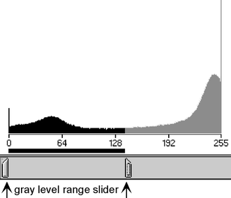

  

  Interactive method of selecting gray levels with graphic slider

• Determine if there are any peaks that correspond to many pixels within a specific gray-level range using a gray-level histogram (Fig. 14).

  Fig. 14

  

  Thresholding gray levels in an image by selecting the gray-level peaks that are characteristic of the features of interest

Interactive selection and histogram characteristic-peaks thresholding methods are used frequently, sometimes together, depending on the particular type of image being viewed. Automatic thresholding often uses the histogram peaks method to determine where to set the gray-level ranges for image segmentation. However, when using automatic thresholding, the user must be careful because changing overall brightness or artifacts, or varying amounts of foreground features, can change the location and the relative size of the peaks. Some advanced algorithms can overcome these variations.

There are more issues to consider when thresholding color images for features of interest. Most systems use red, green, and blue (RGB) channels to establish a color for each pixel in an image. It is difficult to determine the appropriate combination of red, green, and blue signals to distinguish features. Some systems allow the user to point at a series of points in a color image and automatically calculate the RGB values, which are used to threshold the entire image. A better methodology than RGB color space for many applications is to view a color image in hue, intensity, and saturation (HIS) space. The advantage of this method is that color information (hue and saturation) is separated from brightness (intensity). Hue essentially is the color a user observes, while the saturation is the relative strength of the color. For example, translating “dark green” to an HIS perspective would use dark as the level of saturation (generally ranges as a value between 0 and 100%) and green as the hue observed. While saturation describes the relative strength of color, intensity is associated with the brightness of the color. Intensity is analogous to thresholding of gray values in black and white space. Hugh, intensity, and saturation space also is described as hue, lightness, and saturation (HLS) space, where L quantifies the dark-light aspect of colored light.

Nonuniform Segmentation

Selecting the threshold range of gray levels to segment foreground features sometimes results in overdetecting some features and underdetecting others. This is not only due to varying brightness across an image but also is often due to the gradual change of gray levels while scanning across a feature. Delineation enhancement is a useful gray-level enhancement tool in this situation (Fig. 15). This algorithm processes the pixels that surround features by transforming their gradual change in gray level to a much steeper curve. In this way, as features initially fall within the selected gray-level range, the apparent size of the feature will not change much as a wider band of gray levels is selected to segment all features.

Fig. 15

Delineation filter enhances feature edges by sharpening the transition of gray values considerably, providing more leeway when thresholding. a Magnified original gray-level image of particles showing gradual transition of gray levels along the feature edges. b The same image after using a delineation filter

There are other gray-level image processing tools that can be used to delineate edges prior to segmentation and to improve contrast in certain regions of an image, and their applicability to a specific application can be determined by experimenting with them.

Watershed Segmentation

Watershed transformations are iterative processes performed on images that have space-filling features, such as grains. The enhancement usually starts with the basic eroded point or the last point that exists in a feature during successive erosions, often referred to as the ultimate eroded point. Erosion/dilation is the removal and/or addition of pixels to the boundary of features based on neighborhood relationships. The basic eroded point is dilated until the edge of the dilating feature touches another dilating feature, leaving a line of separation (watershed line) between touching features.

Another much faster approach is to create a Euclidean distance map (EDM), which assigns successively brighter gray levels to each dilation iteration in a binary image [2]. The advantage of this approach is that the periphery of each feature grows until impeded by the growth front of another feature. Although watershed segmentation is a powerful tool, it is fraught with application subtleties when applied to a wide range of images. The reader is encouraged to refer to Refs [2] and [3] to gain a better understanding of the proper use and optimization of this algorithm and for a detailed discussion on the use of watershed segmentation in different applications.

Texture Segmentation

Many images contain texture, such as lamellar structures, and features of widely varying size, which may or may not be the features of interest. There are several gray-level algorithms that are particularly well suited to images containing texture because of the inherent frequency or spatial relationships between structures. These operators usually transform gradually varying features (low frequency) or highly varying features (high frequency) into an image with significantly less texture.

Algorithms such as Laplacian, Variance, Roberts, Hurst, and Frei and Chen operators often are used either alone or in combination with other processing algorithms to delineate structures based on differing textures. Methodology to characterize banding and orientation microstructures of metals and alloys is covered in ASTM E 1268 [4].

Pattern-Matching Algorithms

Pattern-matching algorithms are powerful processing tools used to discriminate features of interest in an image. Usually, they require prior knowledge of the general shape of the features contained in the image. For instance, if there are cylindrical fibers orientated in various ways within a two-dimensional section of a composite, a set of boundaries can be generated that correspond to the angles at which a cylinder might occur in three-dimensional space. The resulting boundaries are matched to the actual fibers that exist in the section, and the resulting angles are calculated based on the matched patterns (Fig. 16). In general, pattern-matching algorithms are used when required measurements cannot be directly made or calculated from the shape of a binary feature of interest.

Fig. 16

Pattern matching used for reconstructing glass fibers in a composite. a Bright-field image of a glass fiber composite with several broken fibers. b Computer-generated image after pattern matching, which reconstructs the fibers enabling the quantification of the degree of fiber breakage after processing

Binary Image Processing

Boolean Logic

Binary representation of images allows simple analysis of features of interest while disregarding background information. There are many algorithms that operate on binary images to correct for imperfect segmentation. The use of Boolean logic is a powerful tool that compares two images on a pixel-by-pixel basis and then generates an output image containing the result of the Boolean combination. Four basic Boolean operations are:

• AND

• OR

• Exclusive OR (XOR)

• NOT

These basic four often are combined in various ways to obtain a desired result, as illustrated in Fig. 17.

Fig. 17

Examples of Boolean operators using two images

A simple way to represent Boolean logic is using a truth table, which shows the criteria that must be fulfilled to be included in the output image. When comparing two images, the AND Boolean operation requires that the corresponding pixels from both images be ON (1 = ON, 0 = OFF). Such a truth table would look like:

	AND
Image A	Image B	Output
1	1	1
1	0	0
0	1	0
0	0	0

If a pixel is ON in one image and OFF in another, the resulting pixel will be OFF after the AND Boolean operator is applied. The OR operator requires only that one or the other corresponding pixel from either image be ON to yield a pixel which is ON. The XOR operator produces an ON pixel as long as the corresponding pixels are different; i.e., one is ON and one is OFF. If both the pixels are ON or OFF, then the resulting output will be an OFF value. The NOT operator is simply the inverse of an image, but when used in combination with other Boolean operators can yield interesting and useful results.

Some other truth tables are shown below:

	OR
Image A	Image B	Output
1	1	1
1	0	1
0	1	1
0	0	0

	XOR
Image A	Image B	Output
1	1	0
1	0	1
0	1	1
0	0	0

An important use of Boolean operations is combining multiple criteria, including spatial relationships, multiphase relationships with various materials, brightness differences, and size or morphology within a set of images. It is important that the order and grouping of the particular operation be maintained when designating a particular sequence of Boolean operations.

Feature-based Boolean logic is an extension of pixel-based Boolean logic in that individual features, rather than individual pixels, are compared between images (Fig. 18). The resultant image contains the entire feature instead of just the parts of a feature that are affected by the Boolean comparison. Feature-based logic uses artificial features, such as geometric shapes, and real features, such as grain boundaries, to ascertain information about features of interest.

Fig. 18

Feature-based Boolean logic operates on entire features when determining whether a feature is ON or OFF. This example shows the result when using the AND Boolean operator with images A and B from Fig. 17. An image B outline is shown for illustrative purposes

There are a plethora of uses for Boolean operators on binary images and also in combination with gray-scale images. Examples include coating thickness measurements, stereological measurements, contiguity of phases, and location detection of features.

Morphological Binary Processing

Beyond combining images in unique ways to achieve a useful result, there also are algorithms that alter individual pixels of features within binary images. There are hundreds of specialized algorithms that might help particular applications and merit further experimentation [2, 3]. Several of the most popular algorithms are mentioned below.

Hole Filling

Hole filling is a common tool that removes internal “holes” within features. For example, one technique completely fills enclosed regions of features (Fig. 19a, b) using feature labeling. This identifies only those features that do not touch the image edge, and these are combined with the original image using the Boolean OR operator to reconstruct the original inverted binary image with the holes filled in. There is no limit on how large or tortuous a shape is. The only requirement for hole filling is that the hole is completely contained within a feature.

Fig. 19

Effects of different hole-filling methods. a Transmitted-light image containing an array of glass particles with some interstitial clear regions within the particles. b Same image after the application of the hole-filling algorithm with dark gray regions showing the filled regions. Identified areas 1, 2, and 3 show erroneously filled regions due to the arrangement of particles. c Inverted or negative of the first image, which treats the original interstitial holes as individual features. d Image after removing features below a certain size and inverting the image to its original binary order with only interstitial holes filled

A variation of this is morphological-based hole filling. In this technique, the holes are treated as features in the inverted image and processed in the desired way before inverting the image back. For example, if only holes of a certain size are to be filled, the image is simply inverted, features below the desired size are eliminated, and then the image is inverted back (Fig. 19a, c, d). It also is possible to fill holes based on other shape criteria.

Erosion and Dilation

Common operations that use neighborhood relationships between pixels include erosion and dilation. These operations simply remove or add pixels to the periphery (both externally and internally, if it exists) of a feature based on the shape and location of neighborhood pixels. Erosion often is used to remove extraneous pixels, which may result when overdetection during thresholding occurs, because some noise has the same gray-level range as the features of interest. When used in combination with dilation (referred to as “opening”), it is possible to separate touching particles. Dilation often is used to connect features by first dilating the features followed by erosion to return the features to their approximate original size and shape (referred to as “closing”).

Most image analysis systems allow the option of using several neighborhood-kernel patterns (Fig. 20) and also allow selection of the number of iterations used. However, great care must be exercised when using these algorithms because the feature shape (especially for small features) can be significantly different from the original feature shape. Parameter selection can dramatically affect features in the resulting image because if too many iterations are used relative to the size of the feature, it can take on the shape of the neighborhood pattern used (Fig. 21). However, some very useful results can be achieved when using the right erosion/dilation kernel shape. For instance, using a vertical shape closing in a binary image of a surface can remove edges that fold over themselves (Fig. 22), which allows determination of the roughness of an interface.

Fig. 20

Examples of the effects of erosion on a feature using kernels of various shapes and the associated shape of a single pixel after dilation using the same kernel

Fig. 21

Particle with elongated features showing the effect of using a number of octagonal-opening (erosion followed by a dilation) iterations

Fig. 22

Use of a vertical shape closing in a binary image. a Reflected-light image of a coating having a tortuous interface. b Binary image of coating. c Binary image after hole filling and removal of small unconnected features. d Equally spaced vertical lines overlaid on the binary image. e Result after a Boolean AND of the lines and the binary image. f Image after vertical closing of 35 cycles, which closes off overlapping features of the interface for measuring roughness. g Binary image showing the lines before (dark gray) and the line segments filled in after closing (black). h Vertical lines overlaid on the original lightened gray-level image

Skeletonization, Skeleton by Influence Zones (SKIZ), Pruning, and Convex Hull

A specialized use of erosion that prevents the separation of features while eroding away pixels is called skeletonization, or thinning. This operation is useful when thinning thick, uneven feature boundaries. Caution is advised when using this algorithm on very thick boundaries because the resulting skeleton can change dramatically depending on the existence of just a few pixels on an edge or within a feature.

SKIZ, a variation of skeletonization, operates by simultaneously growing all features in an image (or eroding the background) to the extent possible given the zones of influence of growing features (Fig. 23). This is analogous to nearest-neighbor determinations because drawing a line segment from the edge of one feature to the edge of an adjacent feature results in a midpoint, which is the zone of influence. The result of a SKIZ operation often replicates what an arrangement of grain boundaries looks like. Additionally, it is possible to measure the resulting zone size to quantify spatial clustering or statistics on the overall separation between features.

Fig. 23

Effects of the SKIZ process. a SEM image of a superalloy. b Binary image of gamma prime particles overlaid on the original gray-level image with light gray particles touching the image boundary. c After application of SKIZ showing zones of influence. d Zones with original binary particles overlaid

Occasionally, unconnected boundaries remain after the skeletonization operation and can be removed using a pruning algorithm that eliminates features having endpoints. The convex-hull operation can be used to fill concavities and smooth very jagged skeletons or feature peripheries. Basically, a convex-hull operation selectively dilates concave feature edges until they become convex (Fig. 24).

Fig. 24

Images showing the use of various binary operations on a grain structure. a Original bright-field image of grain structure. b Binary image after removal of small disconnected features. c Binary image after skeletonization with many short arms extending from grain boundaries. d Binary image after pruning. e Binary image after pruning and after three iterations of convex hull to smooth boundaries. f Image showing grain structure after skeletonization of the convex-hulled image

Further Considerations

The binary operations described in this article are only a partial list of the most frequently used operations and can be combined in useful ways to produce an image that lends itself to straightforward quantification of features of interest. Today, image analysis systems incorporate many processing tools to perform automated, or at least fast-feature, analysis. Creativity is the final tool that must be used to take full advantage of the power of image analysis. The user must determine if the time spent in developing a set of processing steps to achieve computerized analysis is justified for the application. For example, if you have a complicated image that has minimal contrast but somewhat obvious features to the human eye and only a couple of images to quantify, then manual measurements or tracing of the features might be adequate. However, the benefit of automated image analysis is that sometimes-subtle feature characterizations can yield answers that the user might never have guessed based on cursory inspections of the microstructure.

References

E. Pirard, V. Lebrun, J.-F. Nivart, Optimal acquisition of video images in reflected light microscopy. Microsc. Anal. 37, 19–21 (1999)
J.C. Russ, The Image Processing Handbook, 2nd edn. (CRC Press, Boca Raton, 1994)
L. Wojnar, Image Analysis, Applications in Materials Engineering (CRC Press, Boca Raton, 1998)
“Standard Practice for Assessing the Degree of Banding or Orientation of Microstructures,” E 1268-94, Annual Book of ASTM Standards, ASTM, 1999
Editor’s Note: Following are more recent references the reader may wish to explore for additional information.
Gegner, J., Ochsner, A.: Digital image analysis in quantitative metallography. Prakt. Metallogr. 38(9), 499-513 (2001)
Ribeiro, L.M.F., Horovistiz, A.L., Jesuíno, G.A., de O Hein, L.R., Abbade, N.P., Crnkovic, S.J.: Fractal analysis of eroded surfaces by digital image processing, Mater. Lett. 56(4), 512-517 (2002)
Wojnar, L., Kurzydlowski, K. J., Szala, J.: Quantitative Image Analysis. In: Vander Voort, G.F., (ed.) Metallography and Microstructures, Vol. 9, ASM Handbook, pp. 403-427, ASM International, Materials Park, OH (2004)
Ochsner, A., Gegner, J., Gracio, J.J.A.: Quantitative determination of microstructural inhomgeneity for directional particle distribution. 42(3), 116-125 (2005)
Collins, T.J.: ImageJ for microscopy. BioTechniques. 43, S25-S30 (July 2007)
Russ, J.C.: The Image Processing Handbook. 5th ed. Taylor & Francis Group (2007)
Wu, Q., Merchant, F., Castleman, K.: Microscope Image Processing, 1st ed. Academic Press (2008)
Limodin, N., Salvo, L., Suéry, M., Delannay, F.: Assessment by microtomography of 2D image analysis methods for the measurement of average grain coordination and size in an aggregate. Scr. Mater. 60(5), 325-328 (2009)
Author information
Authors and Affiliations
Additional information
Reprinted from Practical Guide to Image Analysis, ASM International, Materials Park, OH (2000), copyright © ASM International.
Rights and permissions
About this article
Cite this article
Grande, J.C. Principles of Image Analysis. Metallogr. Microstruct. Anal. 1, 227–243 (2012). https://doi.org/10.1007/s13632-012-0037-5
Published:
Issue Date:
DOI: https://doi.org/10.1007/s13632-012-0037-5