A novel approach to efficient resource allocation in load-balanced cellular networks using hierarchical DRL

Abstract

5G wireless networks require highly spectral-efficient multiple access techniques, which play an important role in determining the performance of mobile communication systems. Multiple access techniques can be classified into orthogonal and nonorthogonal based on the way the resources are allocated to the users. This paper investigates the joint user association and resource allocation problem in an uplink multicast NOMA system to maximize the power efficiency with guaranteeing the quality-of-experience of all subscribers. We also introduce an adaptive load balancing approach that aspires to obtain “almost optimal” fairness among servers from the quality of service (QoS) perspective in which learning automata (LA) has been used to find the optimal solution for this dynamic problem. This approach contains a sophisticated learning automata which consists of time-separation and the “artificial” ergodic paradigms. Different from conventional model-based resource allocation methods, this paper suggested a hierarchical reinforcement learning based frameworks to solve this non-convex and dynamic power optimization problem, referred to as hierarchical deep learning-based resource allocation framework. The entire resource allocation policies of this framework are adjusted by updating the weights of their neural networks according to feedback of the system. The presented learning automata find the $\epsilon$-optimal solution for the problem by resorting to a two-time scale-based SLA paradigm. Numerical results show that the suggested hierarchical resource allocation framework in combination with the load balancing approach, can significantly improve the energy efficiency of the whole NOMA system compared with other approaches.

1 Introduction

The ever-increasing traffic demand in mobile communications has motivated research activities to design the next generation (5G) wireless networks that can offer significant improvements in coverage and user experience (Li et al. 2020). 5G wireless networks require highly spectral-efficient multiple access techniques, which play an important role in determining the performance of mobile communication systems. Multiple access techniques can be classified into orthogonal and nonorthogonal based on the way the resources are allocated to the users (Liu et al. 2018). Recently, related work has emerged to investigate the resource allocation problem in NOMA systems to optimize the system SE. In Khan et al. (2020), game theory is applied to allocate power among users in single-carrier NOMA (SC-NOMA) systems to maximize the revenue of BS. Song et al. (2018) proposed a suboptimal power and channel allocation algorithm combining Lagrangian duality and dynamic programming to maximize the weighted sum rate in a multi-carrier NOMA (MC-NOMA) system. In Wei et al. (2018), for a two-user multiple-input multiple-output (MIMO) NOMA system, the authors propose two power allocation algorithms to maximize the sum capacity under the total power constraint and the minimum rate requirement of weak users.

Many model-based resource allocation algorithms have been proposed to increase EE or other objectives in NOMA systems. The power allocation problems were studied by (Zeng et al. 2017, 2019; Liu et al. 2019a, b; Baidas et al. 2019), and the joint scheduling and power allocation problems were studied by (Cao et al. 2018; Praveenchandar and Tamilarasi 2020; Zhai et al. 2018; Maimó et al. 2019; Fu et al. 2019). However, considering the dynamics and uncertainty that are inherent in wireless communication systems, it is generally hard or even unavailable to obtain the complete knowledge or mathematical model that are required in these conventional resource allocation approaches in practice (Abedin et al. 2018 and Ye and Li 2018). Besides, due to the high computational complexity of these algorithms, they are inefficient or even inapplicable for future communication networks.

Some studies have used deep learning (DL) as a model-free and data-driven approach to reduce the computational complexity with available training inputs and outputs (Celdrán et al. 2019; Huang et al. 2019). As one main branch of machine learning (ML), DL has been used to solve resource allocation problems (Liu et al. 2019a; b; Ye et al. 2019) by training the neural networks offline with simulated data first, then outputting results with the well-trained networks during the online process. However, the correct data set or optimal solutions used for training can be difficult to obtain, and the training process itself is usually time-consuming. Given the above issues, reinforcement learning (RL) (Xu et al. 2018), as another main branch of ML, can be a feasible option for real-time decision-making tasks (e.g., dynamic resource allocation) since in RL the requirements of system model and priori data is widely relaxed. Besides, instead of optimizing current benefits only, RL can generate almost optimal decision policy which maximizes the long-term performance of systems through constant interactions. However, conventional RL algorithms suffer from slow convergence speed and become less efficient for problems with large state and action spaces. Therefore, deep reinforcement learning (DRL), which combines DL with RL, has been proposed to overcome these issues. One famous algorithm of DRL named deep Q-learning (Teng et al. 2020), uses a deep Q network (DQN) which applies deep neural networks as function approximators to conventional RL, and has already been used in many aspects such as power control in NOMA system (Zhao et al. 2019), resource allocation in heterogeneous network (Liu et al. 2018) and internet of things (IoT) (Verhelst and Moons 2017).

However, the main drawback of DQN is that the output decision can only be discrete, which brings quantization error for continuous action tasks (e.g., power allocation). Besides, the output dimension of DQN increases exponentially for multi-action and joint optimization tasks. Fortunately, the recently proposed deep deterministic policy gradient (DDPG) (Qiu et al. 2019) is able to solve these issues. DDPG is an enhanced version of the deterministic policy gradient (DPG) algorithm (Xie and Zhong 2020) based on the actor-critic architecture, which uses an actor network to generate a deterministic action and a critic network to evaluate the action. DDPG also takes the advantages of experience replay and target network strategies from DQN to improve learning stability, which makes DDPG more efficient for dynamic resource allocation problems.

This research considers the load distribution criterion in hierarchical heterogeneous networks which is very important in the next-generation wireless networks and tries to propose a prominent load balancing approach to be adaptive to multi-layer configured networks. We also investigate the hierarchical resource allocation problem in an uplink NOMA system. Motivated by the aforementioned considerations, we present a dynamic framework to improve the long-term energy efficiency of the NOMA system while ensuring a minimum data rate of all subscribers. The first part of the framework is fully based on the dynamic model of DQN, while the second part of the framework combines the advantages of DQN and DDPG considering the load balancing constraints. Based on the DRL methods they use, we refer to this framework as the continuous DRL-based resource allocation, the continuous DRL based resource allocation (CDRA) framework.

The main idea of this paper is based on a claim which the performance of NOMA resource allocation schemes can significantly increase joining with stochastic-based load balancing approaches. This research mainly investigates about the functionality of a prominent resource allocation scheme empowered with an effective load balancing approach in NOMA heterogeneous wireless networks. In this regard, we first interpret a multi agent-based resource allocation scheme using DRL, which has been presented by Li et al. After presenting an adaptive load balancing approach, we prove that the performance of the integrated scheme will significantly increase from the total network energy consumption, forced termination probability, and resource utilization rate perspectives.

The rest of this paper is organized as follows. Section 2 introduces the system model and problem formulation of the uplink NOMA system. Section 3 is relevant to the discrete and continues resource allocation framework. And in Sect. 4, the load balancing approach for dynamic resource allocation is proposed. The simulation results are given in Sect. 5, and final conclusions in Sect. 6.

2 System model and assumptions

As shown in Fig. 1, we consider a user association and resource allocation system considering NOMA channels in which, one base station (BS) considered at the center point of the macro cell and M users scattered randomly in the covered area. The UEs have randomly movement with a velocity of v within the macro cell covered radius. The total provided bandwidth will be shared equally to K orthogonal carriers, so the interference among carriers is harmful. The set of users and carriers are demonstrated as $\mathfrak{m}=\{\mathrm{1,2},\ldots,M\}$ and $\mathcal{K}=\{\mathrm{1,2},\ldots ,K\}$. Suppose each carrier can support two UEs with the highest level of channel quality at a same time, ${b}_{k,m}\left(t\right)$ represents the carrier allocation factor on time-slot (TS) t, in which ${b}_{k,m}\left(t\right)=1$ illustrates that carrier k is allocated to UE m on time slot t, otherwise ${b}_{k,m}\left(t\right)=0$. Hence, the superposition coded signal transmitted on subchannel k is as Eq. (1).

Fig. 1

User association and resource allocation system considering NOMA channels

From the performance assessment perspective, based on the indicated system model, the system functionality can be represented as the following: $\mathrm{S}=\{(\mathrm{i},\mathrm{j},\mathrm{k},\mathrm{m},\mathrm{n})\mid \mathrm{i}\ge 0,\mathrm{i}\ge 0,\mathrm{i}+\mathrm{j}+\mathrm{k}\le \mathrm{C},0\le \mathrm{m}\le \mathrm{M},0\le \mathrm{n}\le \mathrm{N}\}$

All of the steady states can be categorized in some different classes based on the queues’ condition and the available resources. In this stage, each state’s manner should be investigated and the equivalent formulation is obtained. In this scenario, we apply the presented queueing method in (Zhai et al. 2018; Maimó et al. 2019) in which we need Boolean indexes in order to study interaction between different states.

All of the probable states we can consider for the scenario are distinct but to simplify the deployment of the scenario, we consider only four states Si (i = 1, 2, 3, 4) so as S = S1 ∪ S2 ∪ S3 ∪ S4 we can denote the four mentioned states as below cases:

$$\begin{array}{l}{S}_{1}=\{(i,j,k,m,n)\mid i=0;j=0;k=0;m=0;n=0\}\\ {S}_{2}=\{(i,j,k,m,n)/0<(i+j+k)<C;m=0;n=0\}\\ {S}_{3}=\{(i,j,k,m,n)/0<(i+j+k)=C;m=0;n=0\}\\ {S}_{4}=\{(i,j,k,m,n)/C<(i+j+k+n+m)\le (C+M+N);0\le m\le M;0\le n\le N\}\end{array}$$

in the following, we should interpret these four steady states and try to find their equivalent formulations.

$${x}_{k}=\sum_{m = 1}^{M}{b}_{k,m}\left(t\right)\sqrt{{ P}_{k,m}\left(t\right)}{ d}_{k,m}\left(t\right)+{\beta }_{k,m}\left(t\right)$$

(1)

where ${d}_{k,m}\left(t\right)$ and ${P}_{k,m}\left(t\right)$ illustrate the data symbol and transmission power of UE m on carrier k, and ${d}_{k,m}\left(t\right)$ meets the constraint of ${\mathbb{E}}\left[{\left|{d}_{k,m}(t)\right|}^{2}\right]=1$ in which ${\mathbb{E}}\left[\cdot \right]$ denotes the expectation and $\left|.\right|$ shows the absolute degree operation. Note that we have applied queuing model for different QoS-class of data as shown in Fig. 2.

Fig. 2

Applied queuing model for different QoS-class of data

It should be noted that according to the described framework, overall normalized balancing formulation will be achievable through equality (12)

$$\pi Q=0;\text{ and }\sum_{\forall S} {\pi }_{i,j,k,m,n \, = \, 1}$$

In this formulation, ${g}_{k,m}\left(t\right)$ demonstrate the fast Rayleigh fading between base station and UE m on carrier k, which can be calculated as ${g}_{k,m}\left(t\right)=\sqrt{{\beta }_{k,m}\left(t\right)}{h}_{k,m}\left(t\right)$, in which ${\beta }_{k,m}\left(t\right)$ is the fast Rayleigh fading factor supposed to be fixed during one specific time slot but varies over different time slots, and ${h}_{k,m}\left(t\right)$ represents the small scale fading with a normal Gaussian distribution ${h}_{k,m}(t)\sim \mathcal{C}\mathcal{N}(\mathrm{0,1})$. So, the corresponding signal received at the base station in time slot t can be mentioned as

$${\mathcal{Y}}_{k,m}\left(t\right)={b}_{k,m}\left(t\right){g}_{k,m}\left(t\right)\sqrt{{p}_{k,m}\left(t\right)}{d}_{k,m}\left(t\right)+\sum_{i \, = \,I,i \, \ne \, m}^{M}{b}_{k,i}\left(t\right)\sqrt{{p}_{k,i}\left(t\right)}{d}_{k,i}\left(t\right)+{{\beta }_{k,m}\left(t\right)z}_{k,m}\left(t\right)$$

(2)

The first part of the formulation (2) indicates the actual sent signal of UE m on carrier k, and the second section of this equation shows received signal related to other UEs on the particular carrier. The last part of the equation also indicates complete gaussian noise with the distribution pattern of ${z}_{k,m}\left(t\right)\sim \mathcal{C}\mathcal{N}\left(0,{\sigma }_{z}^{2}\right)$.

In the assessment stage, in accordance with the defined probability matrix $\pi$ we will be able to determine the performance assessment indexes in order to compare enhanced mobile broadband and massive and machine-type communications from the quality-of-service point of view. During the performance evaluation process, resource utilization process is considered in both enhanced mobile broadband and massive machine-type communications services as the following. At the destination, successive interference cancellation is applied to decode multiple arrival packets concurrently (Pan et al. 2018), so the interference caused by carrier sharing is prohibited. First, the destination decodes the UE with the highest channel quality level, extracts it from the total received signal and then decodes the remaining signal which contains weaker signals. Hence, the SINR of UE m on carrier k can be represented as

$${\Gamma }_{k,m}(t)=\frac{{b}_{k,m}\left(t\right){p}_{k,m}{(t)\left|{g}_{k,m}\left(t\right)\right|}^{2}}{{\sum }_{i \, = \, I,{\left|{g}_{k,m}\left(t\right)\right|}^{2}<{\left|{g}_{k,m}\left(t\right)\right|}^{2}}^{M}{b}_{k,i}\left(t\right){{\beta }_{k,m}\left(t\right)p}_{k,i}\left(t\right){\left|{g}_{k,i}\left(t\right)\right|}^{2}+{\sigma }_{n}^{2}}$$

(3)

With normalized bandwidth, the corresponding data rate is

$${\xi }_{k,m}\left(t\right)=\mathrm{log}\left(1+{\Gamma }_{k,m}\left(t\right)\right)$$

(4)

In the fully-utilized system which the resource is not enough for the congested network, enhanced mobile broadband should send a demand sequence to release some of the basebands’ resource blocks and dedicate the released resources to the coming ultra-reliable and low-latency communications. In this condition, the forced termination probability will be one of the primary assessment indexes applied in the paper. Because limitation of the uplink transmission rate of each UEs, the non-orthogonal multiple access system determines a user level uplink energy efficiency on carrier k which is computed as ratio of throughput to the total power consumption.

$${E}_{k,m}\left(t\right)=\frac{{\xi }_{k,m}\left(t\right)}{{{\beta }_{k,m}\left(t\right)p}_{k,m}{(t)}+{\mathcal{P}}_{m}},$$

(5)

where ${\mathcal{P}}_{m}$ is a certain amount of power consumed by the device of user m itself (such as baseband signal processing, digital to analog converter and transmit filter), and the larger ${E}_{k,m}\left(t\right)$ represents the idea of having more transmit rate while consuming less power. We aim to optimize the EE performance of the whole NOMA system, so the resource allocation problem is formulated as maximizing the sum EE of all users through selecting the subchannel assignment index ${\{b}_{k,m}\left(t\right)\}$ and the allocated power ${\{p}_{k,m}\left(t\right)\}$ of every TS t, that is

$$P1: \underset{\left\{{b}_{k,m}\left(t\right),{p}_{k,m}(t)\right\}}{\mathrm{max}}\sum_{k \, = \,1}^{K}\sum_{m \, = \,1}^{M}{{\beta }_{k,m}\left(t\right)E}_{k,m}(t)$$

(6)

$$S.t. C1:\sum_{k \, = \,1}^{k}{b}_{k,m}\left(t\right){\beta }_{k,m}\left(t\right){p}_{k,m}\left(t\right)\le {p}_{max},\forall m\in M,$$

$$C2:\sum_{k \, = \,1}^{k}{b}_{k,m}\left(t\right){R}_{k,m}\left(t\right)\ge {R}_{min},\forall m\in M,$$

$$C3:{p}_{k,m}\left(t\right)\ge 0,\forall k\in \mathcal{K},m\in M,$$

$$C4:{b}_{k,m}\left(t\right)\in \left\{\mathrm{0,1}\right\},\forall k\in \mathcal{K},m\in M,$$

$$C5:\sum_{k \, = \,1}^{K}{b}_{k,m}\left(t\right)\le 1,\forall m\in M,$$

$$C6:\sum_{m \, = \,1}^{M}{b}_{k,m}\left(t\right)\le C,\forall k\in \mathcal{K},$$

Applying the balancing formulation, the number of enhanced mobile broadband resource blocks which should be released can be calculated by

$$\sum_{\genfrac{}{}{0pt}{}{\forall s}{i+j+k \, = \,C\text{ and }k \, = \,0}} \frac{{\lambda }_{1}j}{C-j}{\pi }_{i,j,k,m,n}$$

where ${P}_{max}$ is the maximum available power of a device for signal transmission. Constraint C1 indicates that the transmit power of any user cannot exceed the power limitation ${P}_{max}$, and C2 is the minimum data rate requirement ${R}_{min}$ for all users to ensure their quality-of-service (QoS). C3 and C4 are the inherent constraints of ${p}_{k,m}\left(t\right)$ and ${b}_{k,m}\left(t\right)$. C5 and C6 suggest that one subchannel can serve no more than C users, while each user can only access to one subchannel at the same time.

The service completion index of enhanced mobile broadband and massive and machine-type communications which can be calculated as final number of completed services is achievable as

$$SC{R}_{1}=\sum_{\forall S} j{\mu }_{2}{\pi }_{i,j,k,m,n}$$

$$SC{R}_{2}=\sum_{\forall S} j{\mu }_{3}{\pi }_{i,j,k,m,n}$$

With deploying the scenario, it’s obvious that for each steady state $(i,j,k,m,n)$ with C number of available discrete resource, $(i+j+k)$ base band units are utilized by ultra-reliable and low-latency communications, enhanced mobile broadband or massive machine-type communications services. So, the utilization rate of enhanced mobile broadband or massive machine-type communications demands can be calculated as:

$$U=\sum_{\forall S} \frac{i+j+k}{C}{\pi }_{i,j,k,m,n}$$

The optimization problem is non-convex and NP-hard, and the global optimal solution is usually difficult to obtain in practice due to the high computational complexity and the randomly evolving channel conditions. More importantly, the conventional model-based approaches can hardly satisfy the requirements of future wireless communication services. Thus, we present the DRL-based frameworks in the following sections to deal with these problems.

From the performance assessment perspective, based on the indicated system model, the system functionality can be represented as the following:

$$\mathrm{S}=\{(\mathrm{i},\mathrm{j},\mathrm{k},\mathrm{m},\mathrm{n})\mid \mathrm{i}\ge 0,\mathrm{i}\ge 0,\mathrm{i}+\mathrm{j}+\mathrm{k}\le \mathrm{C},0\le \mathrm{m}\le \mathrm{M},0\le \mathrm{n}\le \mathrm{N}\}$$

(7)

All of the steady states can be categorized in some different classes based on the queues’ condition and the available resources. In this stage, each state’s manner should be investigated and the equivalent formulation is obtained. In this scenario, we apply the presented queueing method of (Zhai et al. 2018; Maimó et al. 2019) in which we need Boolean indexes in order to study interaction between different states.

All of the probable states we can consider for the scenario are distinct but to simplify the deployment of the scenario, we consider only four states Si (i = 1, 2, 3, 4) so as S = S1 ∪ S2 ∪ S3 ∪ S4 we can denote the four mentioned states as below cases:

$$\begin{array}{l}{S}_{1}=\{(i,j,k,m,n)\mid i=0;j=0;k=0;m=0;n=0\}\\ {S}_{2}=\{(i,j,k,m,n)/0<(i+j+k)<C;m=0;n=0\}\\ {S}_{3}=\{(i,j,k,m,n)/0<(i+j+k)=C;m=0;n=0\}\\ {S}_{4}=\{(i,j,k,m,n)/C<(i+j+k+n+m)\le (C+M+N);0\le m\le M;0\le n\le N\}\end{array}$$

Now we should interpret these four steady states and try to find their equivalent formulations.

The first state (S1): this state is relevant to conditions in which the system is completely empty that in this state we suppose T equal to 0. In this state, none of the base band units are in service and there is no any traffic in C-radio access network. This state can be defined as the initiation state of the system. So, we can define this state as the following:

$${S}_{1}=\{(i,j,k,m,n)\mid i=0;j=0;k=0;m=0;n=0\}$$

Which all of the parameters are 0 and the equivalent equation is as Eq. (8).

$$\left({\lambda }_{1}+{\lambda }_{2}+{\lambda }_{3}\right){\pi }_{\mathrm{0,0},\mathrm{0,0},0}={\pi }_{\mathrm{1,0},\mathrm{0,0},0}+{\pi }_{\mathrm{0,1},\mathrm{0,0},0}+{\pi }_{\mathrm{0,0},\mathrm{1,0},0}$$

(8)

$$\begin{array}{c}{\lambda }_{{S}_{2}{R}_{2}}=\cdots ={\lambda }_{{S}_{N}{R}_{N}}=\lambda /2 \, {\text{a}}{\text{n}}{\text{d}} \, {\lambda }_{{R}_{1}{D}_{1}}={\lambda }_{{R}_{2}{D}_{2}}=\cdots ={\lambda }_{{R}_{N}{D}_{N}}=\lambda /2\\ {\lambda }_{{R}_{0}{R}_{1}}={\lambda }_{{R}_{1}{R}_{2}}=\cdots ={\lambda }_{{R}_{N}{R}_{N-1}}=\lambda ,\lambda =1, \, {\text{a}}{\text{n}}{\text{d}} \, {\gamma }_{th}^{j}={\gamma }_{th}^{1},j\in [1,N].\\ \end{array}$$

The second state 2 (S2): in this condition, we have some requests in C-RAN with the amount of more than zero and less than a predefined threshold (C). In this state the system isn’t face to any congestion and any delay for requests due to queueing. So, consequently the total accessible resource blocks are more than zero and less than the indicated fixed value (C) and all of the queues are completely empty. The equation of the second state can be demonstrated as:

$${S}_{2}=\{(i,j,k,m,n)/0<(i+j+k)<C;m=0;n=0\}$$

The more detail of Eq. (9) shown in the following.

$$\begin{array}{c}\left(i{\mu }_{1}+{\lambda }_{1}+j{\mu }_{2}+{\lambda }_{2}+k{\mu }_{3}+{\lambda }_{3}\right){\pi }_{i,j,k,\mathrm{0,0}}={\lambda }_{1}{\pi }_{i-1,j,k,\mathrm{0,0}}+\\ (i+1){\mu }_{1}{\pi }_{i+1,j,k,\mathrm{0,0}}+{\lambda }_{2}{\pi }_{i,j-1,k,\mathrm{0,0}}+(j+{1}\text{)} \, {\mu }_{2}{\pi }_{i,j+1,k,\mathrm{0,0}}\\ +{\lambda }_{3}{\pi }_{i,j,k-\mathrm{1,0},0}+(k+1){\mu }_{3}{\pi }_{i,j,k+\mathrm{1,0},0}\end{array}$$

(9)

The third state (S3): this steady state represents the situation that $i+j+k=0$ and $m=n=0$ in which all of the queues are fully empty but the maximum achievable resources applied in radio access network due to cover the requests. This situation can be formulized as Eq. (10).

$$\begin{array}{c}\left(i{\mu }_{1}+{\alpha }_{1}{\lambda }_{1}+j{\mu }_{2}+{\lambda }_{2}+k{\mu }_{3}+{\lambda }_{3}\right){\pi }_{i,j,k,\mathrm{0,0}}={\alpha }_{3}{\lambda }_{1}{\pi }_{i-1,j,k,\mathrm{0,0}}\\ +\left(j{\mu }_{2}+k{\mu }_{3}\right){\pi }_{i,j,k,\mathrm{1,0}}+{\lambda }_{2}{\pi }_{i,j-1,k,\mathrm{0,0}}+k{\mu }_{3}{\pi }_{i,j,k,\mathrm{0,1}}+{\lambda }_{3}{\pi }_{i,j,k-\mathrm{1,0},0}\\ \end{array}$$

(10)

The fourth state (S4): this state is dedicated to all of the remaining possible conditions so as to $0<T>C$, $0<m\le M$, $0<n\le N$. In this state, most parts of the resource blocks are utilized and the requests execution is done based on the queueing process. So, we can formulate this state as Eq. (11).

$$\left(\begin{array}{c}{\alpha }_{6}i{\mu }_{1}+{\alpha }_{1}{\lambda }_{1}+{\alpha }_{7}\left(1-{\alpha }_{6}\right)i{\mu }_{1}+\\ {\alpha }_{6}j{\mu }_{2}+{\alpha }_{7}\left(1-{\alpha }_{6}\right)j{\mu }_{2}+{\alpha }_{8}k{\lambda }_{1}+\\ {\alpha }_{6}k{\mu }_{3}+{\alpha }_{7}\left(1-{\alpha }_{6}\right)k{\mu }_{3}+{\alpha }_{9}{\lambda }_{3}\end{array}\right){\pi }_{i,j,k,m,n}={\alpha }_{3}{\lambda }_{1}{\pi }_{i-1,j+1,k,m-1,n}+{\alpha }_{3}{\lambda }_{1}{\pi }_{i-1,j+1,k,m,n-1}+{\alpha }_{3}{\lambda }_{1}{\pi }_{i,j,k,m-1,n}+{\alpha }_{3}{\lambda }_{1}{\pi }_{i,j,k,m,n-1}$$

(11)

Considering these four defined states and the T-matrix, the below condition should be quarantined.

$$\sum_{\genfrac{}{}{0pt}{}{\forall S}{0<{\pi }_{i,j,k,m,n}<1}} \pi =1$$

According to the described framework, overall normalized balancing formulation will be achievable through equality (12)

$$\pi Q=0;\text{ and }\sum_{\forall S} {\pi }_{i,j,k,m,n=1}$$

(12)

In the assessment stage, in accordance with the defined probability matrix $\pi$ we will be able to determine the performance assessment indexes in order to compare enhanced mobile broadband and massive and machine-type communications from the quality-of-service point of view. During the performance evaluation process, resource utilization process is considered in both enhanced mobile broadband and massive machine-type communications services as the following.

In the fully-utilized system which the resource is not enough for the congested network, enhanced mobile broadband should send a demand sequence to release some of the basebands’ resource blocks and dedicate the released resources to the coming ultra-reliable and low-latency communications. In this condition, the forced termination probability which is represented as PF1 can be calculated as

$${P}_{{F}_{1}}=\frac{the \, average \, rate \, of \, terminated \, eMBB}{the \, eMBB \, admitted \, rate}$$

Applying the balancing formulation, the number of enhanced mobile broadband resource blocks which should be released can be calculated by

$$\sum_{\genfrac{}{}{0pt}{}{\forall s}{i+j+k = C\text{ and }k \,= \, 0}} \frac{{\lambda }_{1}j}{C-j}{\pi }_{i,j,k,m,n}$$

The final enhanced mobile broadband rate is equal to λ2(1 − PB2). Therefore, the forced termination probability obtains via Eqs. (13) and (14).

$$P{F}_{1}=\sum_{\genfrac{}{}{0pt}{}{\forall \mathrm{S}}{i+j+k \,= \, C\text{ and }k \,= \, 0}} \frac{{\lambda }_{1}j}{(C-j){\lambda }_{2}\left(1-P{B}_{2}\right)}{\pi }_{i,j,k,m,n}$$

(13)

$$P{F}_{2}=\sum_{\genfrac{}{}{0pt}{}{\forall \mathrm{S}}{i+j+k \,= \, C\text{ and }n \,= \, N}} \frac{{\lambda }_{1}k}{(C-j){\lambda }_{3}\left(1-P{B}_{2}\right)}{\pi }_{i,j,k,m,n}$$

(14)

The service completion index of enhanced mobile broadband and massive and machine-type communications which can be calculated as final number of completed services is achievable through Eqs. (15) and (16) consequently.

$$SC{R}_{1}=\sum_{\forall S} j{\mu }_{2}{\pi }_{i,j,k,m,n}$$

(15)

$$SC{R}_{2}=\sum_{\forall S} j{\mu }_{3}{\pi }_{i,j,k,m,n}$$

(16)

With deploying the scenario, it’s obvious that for each steady state $(i,j,k,m,n)$ with C number of available discrete resource, $(i+j+k)$ base band units are utilized by ultra-reliable and low-latency communications, enhanced mobile broadband or massive machine-type communications services. So, the utilization rate of enhanced mobile broadband or massive machine-type communications demands can be calculated as:

$$U=\sum_{\forall S} \frac{i+j+k}{C}{\pi }_{i,j,k,m,n})$$

(17)

One of the measurement indexes we select to the assessment of our model is average transmission delay for both enhanced mobile broadband or massive machine-type communications services. As mentioned before, each demand has own distinct queue process based on its quality-of-service thresholds and having different delays for different demands is inevitable. In this scenario, we assume queue length of enhanced mobile broadband or massive machine-type communications as ${L}_{1}$ and ${L}_{2}$ and the mean value of enhanced mobile broadband service $({D}_{1})$ and the mean value of massive machine-type communications $({D}_{2})$ is achievable as:

$${D}_{1}=\frac{{L}_{1}}{{\lambda }_{1}}$$

(18)

which

$${L}_{1}\sum_{\genfrac{}{}{0pt}{}{\forall S}{0\le m\le M}} m{\pi }_{i,j,k,m,n}$$

It should be noted that in calculation of delay for massive machine-type communications demands, all of the interrupts must be calculated in addition to the usual transmission delay. So ${D}_{2}$ changes to:

$${D}_{2}=\frac{{L}_{2}}{{\lambda }_{3}+{R}_{Interrupt}}$$

(19)

In which,

$${L}_{2}={\sum }_{\begin{array}{c}\forall s\\ 0\le n\le N \end{array}}n{\pi }_{i,j,k,m,n}\text{ and }{R}_{\text{Interrup}}=\sum_{\genfrac{}{}{0pt}{}{\forall \mathrm{s}}{\begin{array}{c}i+j+k=C \, \\ \nu <C\end{array}}} \frac{{\lambda }_{1}k}{C-v}{\pi }_{i,j,k,m,n}$$

3 Hierarchical resource allocation

This part of the paper allocated to present the structure of the hierarchical framework called CDRA, in which we applied the same carrier allocation DQN unit based on the introduces framework in the former section to select the best carrier, and subsequently application of a DDPG unit to result in the transmission power of all UEs as shown in Fig. 3. First, we briefly introduce the framework of DDPG. It is not possible for us to use (19) formulation to select actions because the actions considered infinite and consequently Q will also be infinite. In order to find the optimal solution for this problem, the policy gradient approach directly formulates the rule $\pi$ to determine actions, that makes policy gradient the most appropriate method for stablishing continuous reinforcement learning tasks. The formulated framework can be described as Eq. (20) but it should be noted that virtue of the M/M/1 queue, the mean-response time at server i is:

$${MRT}_{i}\left(t\right)=\frac{1}{{\mu }_{i}-{{\beta }_{k,m}\left(t\right)\lambda }_{i}\left(t\right)},$$

where ${\lambda }_{i}\left(t\right)$ is the average arrival rate at server i. If the {${p}_{i}$} are constant or vary slowly over time, then ${\lambda }_{i}\left(t\right)$ can be approximated using ${\lambda }_{i}\left(t\right)={p}_{i}\left(t\right)\lambda$, which is a consequence of the M/M/1 queue model (Zhai et al. 2018).

Fig. 3

Configuration of the dynamic DRL based resource allocation

$${\pi }_{\varnothing }\left(s,a\right)={P}_{r}\left\{\left.a\right|s;\varnothing \right\},$$

(20)

In which $\varnothing$ represents the policy index. This formulation represents the probability of selecting action a considering state s and $\varnothing$. To evaluate the appropriateness of policy ${\pi }_{\varnothing }$, we can utilize the expectation of the cumulative discounted reward to demonstrate the target, which is shown as Eq. (21)

$$J\left({\pi }_{\varnothing }\right)={\int }_{S}{\rho }^{\pi }\left(s\right){\int }_{A}{\pi }_{\varnothing }\left(s,a\right)r\left(s,a\right) {d}_{a} {d}_{s}.$$

(21)

In which, ${\rho }^{\pi }\left(s\right)$ is the distribution of states. Therefore, the goal of PG is to maximize (21) by adjusting the parameters $\varnothing$ in the direction of the performance gradient defined as the following. To proceed with the formulation, let $\alpha (t)$ be the index of the chosen action at time instant t. Then, the value of ${p}_{i}\left(t\right)$ is updated as per the following simple rule (the rules for other values of ${p}_{j}\left(t\right)$, $j\ne i$, are analogous):

$${p}_{i}\left(t+1\right) \leftarrow {p}_{i}\left(t\right)+\theta \left({p}_{max}-{p}_{i}\left(t\right)\right)$$

$$when \, \alpha \left(t\right) = i \, and \, {v}_{i} = 1$$

$${p}_{i}\left(t+1\right) \leftarrow {p}_{i}\left(t\right)+\theta \left({p}_{min}-{p}_{i}\left(t\right)\right)$$

$$when \, \alpha \left(t\right) = j,j \ne i \, and \, {v}_{i} = 1,$$

where $\theta$ is a user-defined parameter 0 < $\theta$  < 1, typically close to zero. Further, ${v}_{i}$ is a reward function indicator defined by:

• ${v}_{i}=1$, reward, if the instantaneous response of the chosen server is under the running moving average of the mean response time, ${s}_{i}\left(t\right)\le \frac{1}{r}{\sum }_{k=1}^{r}{\widehat{s}}_{k}\left(t\right)$.

• ${v}_{i}=0$, penalty, if the instantaneous response of the chosen server exceeds the running moving average of the mean response time, ${\widehat{s}}_{i}\left(t\right)>\frac{1}{r}{\sum }_{k=1}^{r}{\widehat{s}}_{k}\left(t\right)$.

$${\nabla }_{\varnothing }\mathrm{J}\left({\pi }_{\varnothing }\right)= {\int }_{S}^{ }{{\beta }_{k,m}\left(t\right)p}^{\pi }\left(s\right){{\int }_{A}^{ } \nabla }_{\varnothing }{\pi }_{\varnothing }\left(\mathrm{s,a}\right){Q}^{\pi }\left(s,a\right) {d}_{a} {d}_{s}$$

(22)

and Eq. (9) is referred to as the policy gradient theorem (Zhang et al. 2020). However, two main drawbacks are existed in PG methods. First, PG algorithms typically converge to a local optimum rather than the global optimum. Besides, evaluating a policy ${\pi }_{\varnothing }$ is generally inefficient and has high variance, because it requires integration over both state and action spaces (Weisz et al. 2018). To address these problems, the deterministic policy gradient theorem (Wu et al. 2020) is proposed, where an action is deterministically generated by a parameterized policy instead of the probability of actions (20). That is, ${a=\pi }_{\varnothing }\left(s\right)$, and Eq. (25) is rewritten as

$$J\left({\pi }_{\varnothing }\right)={\int }_{S}{{\beta }_{k,m}\left(t\right)p}^{\pi }\left(s\right)r(s,{\pi }_{\varnothing }\left(s\right))ds,$$

(23)

and the corresponding gradient is

$$\begin{aligned} {\nabla }_{\varnothing }\left(s,a\right) &= {\int }_{s}{\beta }_{k,m}\left(t\right){p}^{\pi }\left(s\right){\nabla }_{\varnothing }{\pi }_{\varnothing }(s){\nabla }_{a}{Q}^{\pi }(s,a{\left.)\right|}_{a={\pi }_{\varnothing }(s{)}}ds \hfill \\ & = {E}_{s\sim {p}^{\pi }}\left[{\nabla }_{\varnothing }{\pi }_{\varnothing }\left(s\right){\Delta }_{a}{Q}^{\pi }(s,a{\left.)\right|}_{a={\pi }_{\varnothing \left(s\right)}}\right]+{\beta }_{k,m}\left(t\right ) \end{aligned}$$

(24)

where the deterministic policy gradient (DPG) (28) is a special case of PG (26) when the variance of Eq. (24) reaches 0.

The delay for massive machine-type communications demands, all of the interrupts must be calculated in addition to the usual transmission delay. So ${D}_{2}$ changes to:

$${D}_{2}=\frac{{L}_{2}}{{\lambda }_{3}+{R}_{Interrupt}}$$

In which,

$${L}_{2}={\sum }_{\begin{array}{c}\forall s\\ 0\le n\le N \end{array}}n{\pi }_{i,j,k,m,n}\text{ and }{R}_{\text{Interrup}}=\sum_{\genfrac{}{}{0pt}{}{\forall \mathrm{s}}{\begin{array}{c}i+j+k = C \, \\ \nu <C\end{array}}} \frac{{\lambda }_{1}k}{C-v}{\pi }_{i,j,k,m,n}$$

4 DRL-based load balancing model

In this section we try to apply an effective Load Balancing approach presented by H. Ismail and A. Yazidi which is based on two-time scale LA with barriers into the presented resource allocation approach to empower the suggested approach from the load distribution and load sharing point of views. So, we interpret the archived results of this combination approach after a brief presentation of their load balancing model.

• A. Model

  In this scenario, $r$ servers considered each of which organized as an M/M/1 queue so that entrance probability is modeled as a poisson distribution statistics considering ${\lambda }_{i}$ (Shu and Zhu 2020). The service rate is equal to ${\mu }_{i}$ and the service time has an exponential statistical distribution.

  In this framework, the learning automata will be responsible for dispatching the demand. The learning automata submits the demand to server $i$ which its probability is illustrated as ${p}_{i}\left(t\right)$. In the following of this section we will describe the update process of these learning automata formulations. We can define the update process considering the advantage of M/M/1 queue modelling. Based on this approach, the equation of mean-feedback time relevant to server $i$ will be equal to:

  $${MRT}_{i}\left(t\right)=\frac{1}{{\beta }_{k,m}\left(t\right){\mu }_{i}-{\lambda }_{i}\left(t\right)},$$

  (25)

  In which, ${\lambda }_{i}\left(t\right)$ demonstrates the mean entrance rate of server i. it should be noted that if the {${p}_{i}$} considered as a fixed value or we can ignore its changes, we can consider ${\lambda }_{i}\left(t\right)={p}_{i}\left(t\right)\lambda$, which is as a result of utilizing M/M/1 as a model for the queue (Zhai et al. 2018). We suppose that ${s}_{i}\left(t\right)$ shows the immediate response time at the exact time $t$ at server $i$. considering $\alpha$ as the learning index, to calculate the mean feedback time of server $i$, we have to apply the $exponential-moving-average$ method so that ${\widehat{s}}_{i}\left(t\right)$ shows the approximate mean feedback time.

  The estimation parameter ${\widehat{s}}_{i}\left(t+1\right)$ will be updated right after despatching a demand toward server $i$. this action is done utilizing a dynamic estimator called $exponential-moving-average$ as the following:

  $${\widehat{s}}_{i}\left(t+1\right)= {\widehat{s}}_{i}\left(t\right)+\alpha \left({s}_{i}\left(t\right)-{\widehat{s}}_{i}\left(t\right)\right).$$

  (26)

  The mean feedback time for each other servers remain without change during this process. Here,

  $${\widehat{s}}_{i}\left(t+1\right)= {\widehat{s}}_{i}\left(t\right) for j\ne i , j\in \left[1,n\right].$$

  (27)

  The process of penalty and reward determination for each action is clear. If action $i$ is selected, we have the following instructions relevant to penalty/reward process.

• • Reward if ${\widehat{s}}_{i}\le \frac{1}{r}{\sum }_{k=1}^{r}{\widehat{s}}_{k}$.

• • Penalty if ${\widehat{s}}_{i}>\frac{1}{r}{\sum }_{k=1}^{r}{\widehat{s}}_{k}$.

  Based on this framework, as a back-drop, the proposed approach can be described step-by-step as algorithm 2.

• B. Two-time scale learning automata

  The beginning stage of the preposed approach is related to modification of Markov process from the absorbing form to the ergodic form. Instead of applying the actual constraints of the probability space equal to 0 or 1, we assume that none of the probability factors can be less than a predefined lower bound threshold which we indicated it by ${p}_{min}$ or more than a upper bound threshold denoted as ${p}_{max}$ (Colonius and Rasmussen 2021).

  After definition of these two thresholds, the action-selection stochastic parameter in the learning resolution method will be changed and the optimal value in this scheme will be moving to the determind levels ${p}_{min}$ and ${p}_{max}$ and such a little adjustments can make the framework ergodic and the results will also be completely different compared to other current schemes.

  To obtain such goal, we try to define a minimum level ${p}_{min}$ as the probability factor, in which 0 < ${p}_{min}$< 1 for all selection probability ${x}_{i}$, $1\le i\le r$ and r illustrates the quantity of actions. The optimum value for any selection probability ${p}_{i}$, $1\le i\le r$, is obtained as ${p}_{max}=1-(r-1){p}_{min}$ which it can be considered as a primary target. It will be happened if the other $r-1$ actions are equal to their minimal degree ${p}_{min}$, nevertheless, the action with the highest probability will be equal to ${p}_{max}$. Subsecuently, ${p}_{i}$, for $1\le i\le r$, will take values more than ${p}_{min}$ and less than ${p}_{max}$.

  In this framework, $\alpha (t)$ denotes the parameter of selected action at relevant to time $t$. To proceed with the formulation, let $\alpha (t)$ be the index of the chosen action at time instant t. Hence, ${p}_{i}\left(t\right)$ will be renewed based on the following formulation (the relevant rules for other degrees of ${p}_{j}\left(t\right)$, $j\ne i$, will be similar):

  $${p}_{i}\left(t+1\right) \leftarrow {p}_{i}\left(t\right)+\theta \left({p}_{max}-{p}_{i}\left(t\right)\right)$$
  $$when \, \alpha \left(t\right) = i \, and \, {v}_{i}=1$$
  $${p}_{i}\left(t+1\right) \leftarrow {p}_{i}\left(t\right)+\theta \left({p}_{min}-{p}_{i}\left(t\right)\right)$$
  $$when \, \alpha \left(t\right) = j,j\ne i \, and \, {v}_{i}=1,$$

  In this formulation, $\theta$ demonstrates user level variable 0 < $\theta$  < 1, which is normally close to 0. Also, ${v}_{i}$ indicates a reward function described via:

• • ${v}_{i}=1$, known as the reward, if the imediate feedback of the selected server is less than the $moving-average$ of the average feedback time ${s}_{i}\left(t\right)\le \frac{1}{r}{\sum }_{k=1}^{r}{\widehat{s}}_{k}\left(t\right)$.

• • ${v}_{i}=0$, is known as the penalty, if the imediate feedback of the selected server more than the $moving-average$ of the average feedback time, ${\widehat{s}}_{i}\left(t\right)>\frac{1}{r}{\sum }_{k=1}^{r}{\widehat{s}}_{k}\left(t\right)$.

  This procedure has been summurized in Algorithm 2. As per our description, ${\widehat{s}}\left(t\right)$ indicates the mean immediate feedback times relevant to all the entities during time duration $t$ is exhibited as the following equation:

  $${\widehat{s}}\left(t\right)\le \frac{1}{r}{\sum }_{k=1}^{r}{\widehat{s}}_{k}\left(t\right)$$

  (28)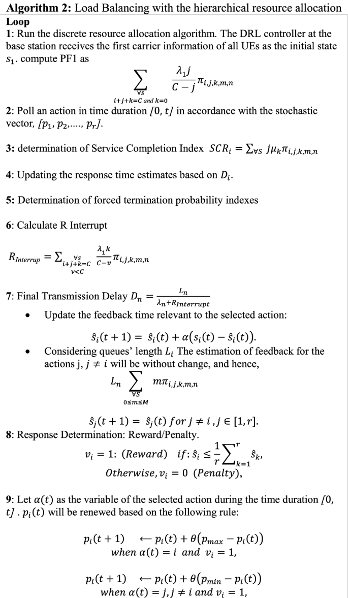

  

  We explained all aspects of the proposed scheme so we should evaluate the performance of this approach compared to the other state of the art schemes during the next part. In the assessment stage, it will be exhibited that as ${p}_{i}\left(t\right)$ enhances, Prob(${s}_{i}\left(t\right)>\widehat{s}(t)$), decreases which this results can be very exciting.

5 Simulation results

In this part of the paper, we tried to evaluate the performance of the presented model compared to some other schemes in a same and identical scenario. The results are simulated in an uplink multi-user NOMA system, where the BS is located at the center of the cell and four users are randomly distributed in the cell with a radius of 400 m. The path loss model is $114+38\mathrm{lg}\left(d\right)+9.2$, where $d(\mathrm{km})$ is the distance between users and BS. The minimum data rate requirement ${R}_{min}=$ 15 bps/Hz, ${\sigma }_{z}^{2}=-174$ dBm and C is set to be 4. If not specified, parameters are set as follows. ${P}_{max}$ = 5 W, ${P}_{0}$ = 25 W, ${T}_{max}$ = 1000 and all users perform random moving with a speed of $\upsilon = 2.5 \, \mathrm{m}/ \mathrm{s}$. For the DDRA framework, each network of all DQN units has three consecutive layers with 64 neurons per layer. The learning rate is 0.015, $\gamma$ = 0.98, $\epsilon$ = 0.9, memory capacity D = 450, weights update interval W = 50 and batch size N = 64. For the CDRA framework, the subchannel assignment DQN unit is the same as the one in the DDRA framework.

In this scenario we consider a single C- radio access network with 45 accessible base band units (i.e., C = 45). We also have assumed three distinct quality of service class for different arrival rate of services which all of the service streams are categorized in one of the following cases:

• Ultra-reliable and low-latency communications.

• Enhanced mobile broadband.

• Massive machine-type communications.

In which we have λ1 = 3, λ2 = 3, λ3 = 6 for the three services respectively. And data rate relevant to each service is μ1 = 0.8, μ2 = 1.0, and μ3 = 0.7. The queue length for two distinct applied queues is 10 (L = 6) and 2 (L = 2) respectively.

In comparison with DL-based approaches in deep learning for effective non-orthogonal multiple access networks, we have compared the performance of the proposed scheme with (Liu et al. 2017; Gui et al. 2018) which Liu et al. (2017) applied a long-short-term memory (LSTM) to detect the channel characteristics automatically. As we mentioned before, evaluation of the resource allocation approach is done both individually (CDRA) and combined with the introduced load balancing approach (CDRA + LB). We can also consider LSTM individually or in combination with RTN method.

In the first round of the assessment, we have deployed three different algorithms in a same scenario in which the assessment index was rate of resource utilization per service rae. As shown in Fig. 4, the combination of CDRA with the suggested load balancing model achieved the best result with the significant difference to other two schemes. In this scenario the effectiveness of the stochastic load balancing method is completely obvious. It has been clear that without empowerment of CDRA, this approach has no any excellence compared to LSTM.

Fig. 4

Resource utilization of ultra-reliable and low-latency communications

In Fig. 5, the evaluation index is the amount of forced termination probability versus arival rate. In this scenario we considered five different algorithms in which CDRA and LSTM are the main algorithms with/without additional methods like as load balancing and RTN. The major target of this plot is to interpret the functionality of each algorithm, when the arrival service rate of massive machine-type communications request with the best QoS class increases. As we mentioned before, in such scenario, evaluation of the queues’ length or queue delays cannot be enough individually and the more effective index which should be investigated in force terminated probability of each services. Based on the obtained results, it is obvious that the combination of CDRA is choosen as the best solution for having least force termination probability. The performance of CDRA can also be better when this algorithm empowered by the load balancing approach.

Fig. 5

Forced termination probability per arrival rate for massive machine-type communications

Figure 6 demonstrated the queuing delay of massive machine-type communications service for various approaches. It shown that CDRA outperforms that of LSTM generally although in some cases when the service arival rate increases, the combination of LSTM and RTN has excellence compared to CDRA. It’s why that when any interrupted requests relevant to the massive machine-type communications join back to its queue, we will face to queue length increasing and in this condition increasing the queueing delay is inevitable.

Fig. 6

Average queue delay of enhanced mobile broadband arrival rate for different approaches

Actually there is a tradeoff between the average queuing delay and the force termination probability but the effect of using the load balancing approach can completely change this process. However, the best solution for this problem is finding the optimal queue length which be able to balance this tradeoff’s parameters.

In Fig. 7, the performance of the proposed CDRA approach and LSTM have been compared from the perspective of total consumption energy for different number of connected subscribers. As it is obvious in this figure, the total consumed energy of LSTM is completely close to CDRA.

Fig. 7

Total network energy consumption (mj) versus the number of connected users (#)

Figure 8 demonstrates the effect of number of resource block on the energy consumption. This result proves that we can decrease the consumed energy by increasing the number of resource blockes. It has been also exhibited that CDRA has better performance than other two DL-based NOMA resource allocation approaches.

Fig. 8

Total energy consumption (mj) versus the number of resource block (#)

6 Conclusion

This paper investigates the joint user association and resource allocation problem in an uplink multicast NOMA system to maximize the power efficiency with guaranteeing the quality-of-experience of all subscribers. We also introduced an adaptive load balancing approach that aspires to obtain “almost optimal” fairness among servers from the quality of service (QoS) perspective in which learning automata (LA) has been used to find the optimal solution for this dynamic problem. Different from conventional model-based resource allocation methods, this paper suggested a hierarchical reinforcement learning-based framework to solve this non-convex and dynamic power optimization problem. The presented learning automata find the $\epsilon$-optimal solution for the problem by resorting to a two-time scale-based SLA paradigm. Numerical results show that the suggested hierarchical resource allocation framework in combination with the load balancing approach, can significantly improve the energy efficiency of the whole NOMA system compared with other approaches. For the DDRA framework, a discrete and distributed multi-DQN strategy is proposed to reduce the output dimension. And for the CDRA framework, we combine the advantages of DQN and DDPG with the load balancing approach to design a joint resource allocation network. Both frameworks are trained jointly to find the optimal subchannel assignment and power allocation policy through constant interaction with the NOMA system. Compared with other alternative approaches, this framework is able to provide better EE under different transmit power limitations, and are applicable in various moving speed conditions by adjusting the parameters of networks, which proves the effectiveness of our proposed frameworks.

References

Abedin SF, Alam MGR, Kazmi SA, Tran NH, Niyato D, Hong CS (2018) Resource allocation for ultra-reliable and enhanced mobile broadband IoT applications in fog network. IEEE Trans Commun 67(1):489–502
Baidas MW, Alsusa E, Hamdi KA (2019) Joint relay selection and energy-efficient power allocation strategies in energy-harvesting cooperative NOMA networks. Trans Emerg Telecommun Technol 30(7):e3593
Cao X, Ma R, Liu L, Shi H, Cheng Y, Sun C (2018) A machine learning-based algorithm for joint scheduling and power control in wireless networks. IEEE Internet Things J 5(6):4308–4318
Celdrán AH, Pérez MG, Clemente FJG, Pérez GM (2019) Towards the autonomous provision of self-protection capabilities in 5G networks. J Ambient Intell Humaniz Comput 10(12):4707–4720
Colonius F, Rasmussen M (2021) Quasi-ergodic limits for finite absorbing Markov chains. Linear Algebra Appl 609:253–288
Fu S, Fang F, Zhao L, Ding Z, Jian X (2019) Joint transmission scheduling and power allocation in non-orthogonal multiple access. IEEE Trans Commun 67(11):8137–8150
Gui G, Huang H, Song Y, Sari H (2018) Deep learning for an effective nonorthogonal multiple access scheme. IEEE Trans Veh Technol 67(9):8440–8450
Huang H, Peng Y, Yang J, Xia W, Gui G (2019) Fast beamforming design via deep learning. IEEE Trans Veh Technol 69(1):1065–1069
Khan WU, Liu J, Jameel F, Sharma V, Jantti R, Han Z (2020) Spectral efficiency optimization for next generation NOMA-enabled IoT networks. IEEE Trans Veh Technol 69(12):15284–15297
Li J, Bao X, Zhang W, Bao N (2020) QoE probability coverage model of indoor visible light communication network. IEEE Access 8:45390–45399
Liu C, Jin Z, Gu J, Qiu C (2017) Short-term load forecasting using a long short-term memory network. In: 2017 IEEE PES innovative smart grid technologies conference Europe (ISGT-Europe), pp 1–6
Liu M, Song T, Gui G (2018) Deep cognitive perspective: resource allocation for NOMA-based heterogeneous IoT with imperfect SIC. IEEE Internet Things J 6(2):2885–2894
Liu P, Li Y, Cheng W, Zhang W, Gao X (2019a) Energy-efficient power allocation for millimeter wave beamspace MIMO-NOMA systems. IEEE Access 7:114582–114592
Liu Y, Yu H, Xie S, Zhang Y (2019b) Deep reinforcement learning for offloading and resource allocation in vehicle edge computing and networks. IEEE Trans Veh Technol 68(11):11158–11168
Maimó LF, Celdrán AH, Pérez MG, Clemente FJG, Pérez GM (2019) Dynamic management of a deep learning-based anomaly detection system for 5G networks. J Ambient Intell Humaniz Comput 10(8):3083–3097
Pan H, Liew SC, Liang J, Shao Y, Lu L (2018) Network-coded multiple access on unmanned aerial vehicle. IEEE J Sel Areas Commun 36(9):2071–2086
Praveenchandar J, Tamilarasi A (2020) Dynamic resource allocation with optimized task scheduling and improved power management in cloud computing. J Ambient Intell Humaniz Comput. https://doi.org/10.1007/s12652-020-01794-6
Qiu C, Hu Y, Chen Y, Zeng B (2019) Deep deterministic policy gradient (DDPG)-based energy harvesting wireless communications. IEEE Internet Things J 6(5):8577–8588
Shu Y, Zhu F (2020) An edge computing offloading mechanism for mobile peer sensing and network load weak balancing in 5G network. J Ambient Intell Humaniz Comput 11(2):503–510
Song Z, Ni Q, Sun X (2018) Spectrum and energy efficient resource allocation with QoS requirements for hybrid MC-NOMA 5G systems. IEEE Access 6:37055–37069
Teng Z, Zhang B, Fan J (2020) Three-step action search networks with deep q-learning for real-time object tracking. Pattern Recogn 101:107188
Verhelst M, Moons B (2017) Embedded deep neural network processing: algorithmic and processor techniques bring deep learning to IOT and edge devices. IEEE Solid State Circuits Mag 9(4):55–65
Wei Z, Zhao L, Guo J, Ng DWK, Yuan J (2018) Multi-beam NOMA for hybrid mmWave systems. IEEE Trans Commun 67(2):1705–1719
Weisz G, Budzianowski P, Su PH, Gašić M (2018) Sample efficient deep reinforcement learning for dialogue systems with large action spaces. IEEE ACM Trans Audio Speech Lang Process 26(11):2083–2097
Wu D, Dong X, Shen J, Hoi SC (2020) Reducing estimation bias via triplet-average deep deterministic policy gradient. IEEE Trans Neural Netw Learn Syst 31(11):4933–4945
Xie D, Zhong X (2020) Semicentralized deep deterministic policy gradient in cooperative StarCraft games. IEEE Trans Neural Netw Learn Syst. https://doi.org/10.1109/TNNLS.2020.3042943
Xu X, Zuo L, Li X, Qian L, Ren J, Sun Z (2018) A reinforcement learning approach to autonomous decision making of intelligent vehicles on highways. IEEE Trans Syst Man Cybern Syst 50(10):3884–3897
Ye H, Li GY (2018) Deep reinforcement learning for resource allocation in V2V communications. In: 2018 IEEE international conference on communications (ICC), pp 1–6
Ye H, Li GY, Juang BHF (2019) Deep reinforcement learning based resource allocation for V2V communications. IEEE Trans Veh Technol 68(4):3163–3173
Zeng M, Yadav A, Dobre OA, Tsiropoulos GI, Poor HV (2017) Capacity comparison between MIMO-NOMA and MIMO-OMA with multiple users in a cluster. IEEE J Sel Areas Commun 35(10):2413–2424
Zeng M, Hao W, Dobre OA, Poor HV (2019) Energy-efficient power allocation in uplink mmWave massive MIMO with NOMA. IEEE Trans Veh Technol 68(3):3000–3004
Zhai D, Zhang R, Cai L, Li B, Jiang Y (2018) Energy-efficient user scheduling and power allocation for NOMA-based wireless networks with massive IoT devices. IEEE Internet Things J 5(3):1857–1868
Zhang K, Koppel A, Zhu H, Basar T (2020) Global convergence of policy gradient methods to (almost) locally optimal policies. SIAM J Control Optim 58(6):3586–3612
Zhao N, Liang YC, Niyato D, Pei Y, Wu M, Jiang Y (2019) Deep reinforcement learning for user association and resource allocation in heterogeneous cellular networks. IEEE Trans Wirel Commun 18(11):5141–5152
Author information
Authors and Affiliations
Corresponding author
Additional information
Publisher's Note
Springer Nature remains neutral with regard to jurisdictional claims in published maps and institutional affiliations.
Rights and permissions
About this article
Cite this article
Rahimi, A., Ziaeddini, A. & Gonglee, S. A novel approach to efficient resource allocation in load-balanced cellular networks using hierarchical DRL. J Ambient Intell Human Comput 13, 2887–2901 (2022). https://doi.org/10.1007/s12652-021-03174-0
Received:
Accepted:
Published:
Issue Date:
DOI: https://doi.org/10.1007/s12652-021-03174-0