
Abstract
Integrated vibration in electrical discharge machining (EDM) plays a key role in achieving high efficiency. High levels of variables can be employed in this approach due to integration. However, simultaneous optimization of the EDM parameters to achieve multi-objectives is still very complex and challenging. Studies on integrated vibration are still in a preliminary stage. This report addresses multi-objective optimization in EDM for SKD61 die steel using low-frequency vibration. MOORA (Multi-objective optimization based on ratio analysis) was chosen to resolve this multi-objective optimization problem. The material removal rate (MRR), tool wear rate (TWR) and surface roughness (SR) were selected as performance measures in the EDM process. An analytical hierarchical process (AHP) was used to determine the weight value of the quality indicators. The results indicate that low-frequency vibrations significantly improve machining efficiency. When the frequency of the vibrations increased, MRR increased significantly such that MRRMAX = 64.48%. TWR and SR are smaller and their increase are given as TWRMAX = 20.3% and SRMAX = 18.47%. MOORA has been identified as a suitable alternative to multi-objective optimization in an EDM process using low-frequency vibrations for an assigned workpiece. The optimum parameters required to achieve the multi-objective were Ton = 25 μs, I = 8 A, Tof = 5.5 μs and F = 512 Hz, at the resultant quality criteria of MRR = 9.564 mm3/min, TWR = 1.944 mm3/min and SR = 3.24 µm with a maximum error of 8.24%.
1 Introduction
The electrical discharge machining (EDM) process has been frequently used to form dies, tool surfaces and in aerospace technology. It is highly effective in the machining of complex geometries in difficult-to-work materials [1]. However, the process parameters in this approach are selected according to the experience of the technicians or based on the user manual. This has resulted in the limited use of EDM. Numerous technical solutions have been proposed such as process optimization, mixing of powder into the EDM-dielectric, and integrated vibration to improve the material removal rate (MRR) [2,3,4]. However, there are many challenges associated with the implementation of this technique, including the integrated vibration system and the mixing of the powder into dielectric solutions. Several statistical techniques have also been applied to solve these challenges using a simpler approach, especially the multi-objective optimization problem [5]. This has contributed to the improvement of the overall efficiency of EDM for practical production.
Integrated vibrations in EDM have been achieved by integrating electrodes or workpieces. The low-frequency vibrations are assigned to electrical arc machining for W9Mo2Cr4V [6]. The results indicate that integrated vibration in the machining process increases MRR by reducing the tool wear and surface roughness (SR). Similar results have been reported for EDM of Inconel-718 via the application of low-frequency vibrations (F = 0–80 Hz) [7]. The results indicated that the increased vibration frequency causes an increase in the MRR by 27.6% and electrical wear rate (EWR) by 6.16%, in addition to a reduction of overcut and taper angle by 31.84% and 18.58%, respectively. The increasing performance measure is associated with the improvement in the flow of chips at various vibrations of electrodes or workpieces in EDM drilling [8]. The assignment of vibrations to μ-EDM results in higher efficiency. The low-frequency vibration (F = 10–70 Hz) is assigned to the workpiece in µ-EDM drilling, which significantly improves the flushing efficiency of the dielectric fluid flow in addition to enhancement of the stability of the machining process. This contributes to a 70% reduction in the machining time relative to conventional EDM [9]. Compared with conventional WEDM, WEDM with low-frequency vibration (F = 0–80 Hz) assigned to an Inconel 718 workpiece demonstrated that MRR is improved by 66.20% and the adhesion of the chip to the machined surface is significantly reduced [10]. Ultrasonic vibrations assigned to the electrodes in EDM have revealed the efficient release of chips [11]. Moreover, vibrations with an ultrasonic frequency of 5 kHz have resulted in an MRR that is six times higher compared with µ-EDM assigned to workpieces in the case of scanning 3D µ-EDM [12]. In EDM with a vibration frequency F = 40 kHz, the MRR and TWR were increased by 47% and 18%, respectively [13].
The efficiency of low-frequency vibrations assigned to electrodes under oil and water dielectric fluids has been examined and evaluated [14]. The results indicate a high MRR (23%) and the minimum TWR decreases in oil and water. Although water was more effective than oil, the surface quality was better in the case of the former [15].
The amplitude and vibration frequency have a strong influence on the productivity and surface quality of the machining process [16]. A low-vibration-frequency EDM was assigned to process SS304 stainless steel. A high MRR, with a reduced TWR, and SR were achieved. Although it is difficult to apply electrical vibrations in μ-EDM compared with conventional EDM, the surface quality is superior under integrated vibration [17]. In addition, low-frequency vibration of the workpiece results in a decrease of short-circuit pulses by 80% and the discharge pulses by 40% during EDM [18]. This leads to a more stable machining process and an increase in MRR, in addition to a considerable decrease in SR.
The integration of vibrations into the EDM process has resulted in a significant improvement in machining efficiency [19]. However, the accuracy of the hole size in μ-EDM needs to be improved. Vibrations contribute to the improvement of the flow velocity of the dielectric fluid, thereby increasing the discharge frequency [20]. This improves machine productivity and reduces the electrode wear rate. Compared with conventional-EDM, the MRR increased by 187.5% and the EWR decreased by 925% when vibrations were assigned to the electrodes [21]. Therefore, vibrations may be assigned to the electrodes or the workpieces to improve the machinability [22]. Few studies have been performed to investigate the effect of the assignment of vibrations to the workpieces in EDM. The results may be limited due to the influence of the material properties and the dimensions of the workpiece [23]. In addition, vibration-assisted EDM is affected by both electrical and non-electrical parameters. Therefore, the analysis and optimization of this parameter is essential and has been shown to contribute to the improvement of machining quality. These investigations are mainly at the preliminary stage and there are few studies on process parameter optimization in vibration-assisted EDM, including the optimization problem. The Taguchi method combined with multi-objective optimization techniques (TOPSIS, GRA, Multi-objective optimization based on ratio analysis—MOORA) has been widely used in EDM, and analytical hierarchical process (AHP) is used to determine the weight of the quality indicators. The result for MOORA is better than that of TOPSIS and GRA [24]. Therefore, AHP–Taguchi–MOORA may be suitable and effective for multi-objective optimization in vibration-assisted EDM. This is a potential area for continued investigations in the future.
This report aims to examine multi-objective optimization of the process parameters in EDM via low-frequency vibrations assigned to an SKD61 workpiece. Process parameters including current (I), pulse-on time (Ton), pulse-off time (Tof) and frequency vibration (F) were selected for examination. MRR and SR were selected as the quality indicators for evaluation. AHP–Taguchi–MOORA was utilized to optimize multiple objectives in this study.
2 Experimental set-up
2.1 Workpiece materials
SKD61 steel is commonly used to manufacture small and medium-sized hot dies and cast dies. The prepared workpiece samples had dimensions of 50 mm length, 10 mm width and 5 mm thickness. Copper (Cu) electrodes with a cylindrical shape with a length of 35 mm and a diameter of 25 mm were used in the EDM process. The sets of process parameters are summarized in table 1. The parameters were determined based on the latest literature review and recommendations for industrial practice.
2.2 Experimental set-up and machine details
The experimental investigations were conducted on a CHEMER EDM machine type CM 323C. The workpiece was attached to the vibration protection fixture of the vibration unit to facilitate stable and accurate transmission of vibrations to the workpiece. Trial runs were performed to evaluate the stability of the system (figure 1). The vibration unit (Model: Exciter 4824, Brüel and Kjær, Denmark) was used to investigate the vibrations. The maximum force generated by the vibrating head was 100 N and the maximum displacement between two peaks was 1 inch when the vibration was set to the lowest frequency. The frequency range of 2–5000 Hz produces oscillations: Sine, pulse and random signals. The amplitude of the vibrations for a chosen frequency value is a = 0.75 µm.

Schematic experimental chart depicting the vibration set-up and data logger.
2.3 Quality indicators and evaluation equipment
MRR: This parameter was calculated based on the volume of material removed per unit time. It is a key parameter that affects the productivity and machining process time. The volume of the removed workpiece was calculated based on the weight of the workpiece before and after machining using the following formula (Eq. 1):
where Wb represents the weight of the workpiece before machining (g) and Wa is the weight of the workpiece after machining (g). The variable “t” is the processing time (min) and ρw represents the density (g/cm3) of the workpiece material. The precise weight of the workpiece was determined using a digital scale (Model: Vibra AJ-203 SHINKO, Japan). The specifications included a maximum weight limit of 200 g with an accuracy of ±0.001 g for repetitions (std. dev.) 10 mg.
Tool wear rate (TWR): The volume of electrode material eroded per minute has a significant effect on the machining precision and cost. The TWR was defined in the same way as the MRR (Eq. 2). The corrosion-defective electrode measurement process was similar to the erosion measurement of the workpiece.
where Tb is the weight of the tool before machining (g) and Ta is the weight after machining (g). The machining time “t” has the unit of minutes (min) and “ρT” is the density of the tool material (g/cm3).
SR: This indicator directly affects the smoothness of the surface after machining, and this will determine the choice of the next machining solution after EDM. The SR was used mainly in EDM in terms of Ra and it is determined by Eq. (3):
where “L” is the sampling length (mm), “h” is the profile curve and “x” is the profile direction. The average SR (Ra) was measured within a length of L = 0.8 mm. The SR (Ra, Rz) was measured using a contact probe (SJ-210)-type profilometer (MITUTOYO, Japan). The evaluation length was 5 mm. Measurements were acquired for each test sample and the average value of each measurement was considered. In addition, a scanning electron microscope (Jeol-6490 JED-2300, JEOL, Japan) was used to observe the surface morphology.
3 Experimental method
The Taguchi method is frequently adopted to optimize the EDM parameters. Taguchi has numerous advantages such as its ability to accommodate many parameters, the arbitrary choice of its levels and the smaller number of experiments. In addition, Taguchi is suitable for studying undefined machining methods or machining methods at an early stage. In this study, 4 inputs parameters, each with 3 levels, were utilized. The degree of freedom of the experiments (8 dof) and Taguchi’s appropriate orthogonal matrix (L9) were chosen according to table 2.
Multi-objective optimization: Brauers and Zavadskas [25] proposed the MOORA method to simultaneously optimize the opposite objectives (n ≥ c2). The calculation steps are as follows [26].
-
Step 1: In multi-objective optimization, a criterion was defined to ensure the purpose of the optimization. The alternatives and their characteristics were classified in the initial stage.
-
Step 2: The determination matrix was built from the initially selected criteria. In this case, “m” depicts the number of alternatives and “n” is the number of quality indicators to be examined. The determination matrix of m × n can be expressed as Eq. (4):
$$ {\text{X = }}\left[ {\begin{array}{*{20}c} {{\text{x}}_{ 1 1} } & {{\text{x}}_{ 1 2} } & .& {{\text{x}}_{{ 1 {\text{j}}}} } & {{\text{x}}_{{ 1 {\text{n}}}} } \\ {{\text{x}}_{ 2 1} } & {{\text{x}}_{ 2 2} } & .& {{\text{x}}_{{ 2 {\text{j}}}} } & {{\text{x}}_{{ 2 {\text{n}}}} } \\ .& .& .& .& .\\ {{\text{x}}_{\text{i1}} } & {{\text{x}}_{\text{i2}} } & .& {{\text{x}}_{\text{ij}} } & {{\text{x}}_{\text{in}} } \\ .& .& .& .& .\\ {{\text{x}}_{\text{m1}} } & {{\text{x}}_{\text{m2}} } & .& {{\text{x}}_{\text{mj}} } & {{\text{x}}_{\text{mn}} } \\ \end{array} } \right], $$(4)where Xij is the value of the jth quality indicator for an ith alternative.
-
Step 3: The performance measure and normalization of the determination matrix was transformed into a non-dimensional matrix to compare all quality indicators. The beneficial and non-beneficial indicators do not affect the normalization of the determination matrix; therefore, its technical characteristics are necessary. This method of normalization is performed in Eq. (5):
$$ x_{ij}^{*} = \frac{{x_{ij} }}{{\sqrt {\sum\nolimits_{i = 1}^{m} {x_{ij}^{2} } } }}, $$(5)where x*ij is the normalized quality indicator value at the ith row and jth column (i = 1, 2, 3, …, m and j = 1, 2, …, n). x*ij is between 0 and 1.
-
Step 4: In this step, normalization performance measures are added to the beneficial criteria and subtracted from the non-beneficial criteria for evaluation. The results are calculated using Eq. (6):
$$ Z_{i} = \sum\nolimits_{j}^{g} {x_{ij}^{*} } - \sum\nolimits_{j = g + 1}^{n} {x_{ij}^{*} } $$(6) -
Step 5: Weight is assigned to the normalized quality indicators to assess the objectives; “wj” is assigned to each quality indicator that is calculated using Eq. (7):
$$ Z_{i} = \sum\nolimits_{j}^{g} {w_{j} } x_{ij}^{*} - \sum\nolimits_{j = g + 1}^{n} {w_{j} } x_{ij}^{*} , $$(7)where “wj” is the weight assigned to each quality characteristic and the total weighted values of all quality indicator must satisfy Eq. (8):
$$ \sum\limits_{j = 1}^{n} {{\text{w}}_{j} } = 1. $$(8) -
Step 6: The ranking for overall assessment is assigned based on the value of the priority index. Ranking is performed according to the descending value of “Zj.” The experiment with the highest value of Zj is the best, and it provides the optimum cutting parameters (optimal solution).
4 Results and discussion
4.1 Calculated by combined MOORA and AHP
-
Step 1. The MOORA method was used to simultaneously optimize the three quality criteria: MRR, TWR and SR.
-
Step 2. The selected criteria are sorted in a matrix form:
$$ {\text{X}} = \left[ {\begin{array}{*{20}c} {{\text{MRR}}_{ 1} } & {{\text{SR}}_{ 1} } \\ .& .\\ .& .\\ .& .\\ {{\text{MRR}}_{ 9} } & {{\text{SR}}_{ 9} } \\ \end{array} \begin{array}{*{20}c} {{\text{TWR}}_{ 1} } \\ .\\ .\\ .\\ {{\text{TWR}}_{ 9} } \\ \end{array} } \right]. $$ -
Step 3. Standardize the matrix: the decision matrix is normalized using Eq. (5) and shown in table 3.
Table 3 Transformation matrix of quality criteria. -
Step 4. To assign the weight value to each quality indicator, a priority criterion “Wj” was selected. The average calculation method was used to determine the weight of the quality indicators [27]. In this study, identified comparison pairs and normalization are shown in table 4. Wj is determined using the AHP method based on the values given in table 5.
Table 4 Pairwise comparison matrix of the main criteria concerning the goal. Table 5 Value of the weight. -
Step 5. Assignment of the weights to the selected criterion for the normalized matrix.
-
Step 6. Ranked index by the MOORA method: table 6 indicates that the 8th experiment has the highest Zj value among all the quality criteria (figure 2). Therefore, the 8th experiment provides the optimal process parameters: Ton = 25 μs, I = 8 A, Tof = 5.5 μs and F = 512 Hz. The corresponding optimal process parameters and the quality criteria are MRR = 9.564 mm3/min, TWR = 1.944 mm3/min and SR = 3.24 µm. Table 7 shows the contribution-wise ranking of each process parameter. In addition, I has the highest contribution (rank 1), followed by F and Tof, whereas Ton has the smallest contribution.
Table 6 Normalization matrix of criteria with weights. Figure 2 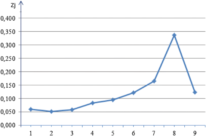
Ranking of Zj.
Table 7 Response table for the means.

4.2 Effect of process parameters on Zj
The effect of each process parameter on the quality indicator is shown in figures 3 and 4, as follows.

Main effects on the plot of Zj quality characteristic.

Effect of I on MRR, SR and TWR.
Figure 3a depicts the effect of current (I) on the quality measures MRR, SR and TWR. An increase of “I” from 3 to 8 A resulted in a robust increase in the quality measures. This rapid increase of the quality indicators may be attributed to the improved quality measures, Zj, due to the low-frequency vibration of the workpiece. In comparison with Zj at I = 3 A, the value of Zj at I = 8 A has the largest increase of 238.80%. An increase of “I” led to an increase of MRR, Ra and TWR, due to the increase of the electric spark energy. The rapid increase of Zj may be due to the significant increase in MRR compared with the increase in SR and TWR (figure 4). The largest increase in the quality indicators was followed by an increase in MRR of 357.81%, an increase in TWR of 65.50% and an increase in SR of 55.57%. In addition, MRR had a higher priority weight than SR and TWR, so the effect of MRR on Zj was the highest.
Figure 3b displays the effect of the pulse-on time (Ton) for a variation from 12 to 50 µs to evaluate the effect on the Zj quality parameters. The Zj is largest at Ton of 25 µs and smallest at 50 µs. The change of MRR, TWR and SR is shown in figure 5. The change of Ton affected the timing of the spark discharge and this parameter has the same effect as a change of the current. However, the degree of influence of Ton on the spark energy is much smaller than that of I. The variation of Ton from 25 to 50 µs resulted in the reduction of MRR, SR and TWR. The reduction of Zj may be associated with the high value of Ton, which leads to a reduced Tof. Processing in EDM becomes unstable and a short-circuit phenomenon may appear. The significant change of the quality indicators includes MRR ≈ 22.90%, SR ≈ 14.76% and TWR ≈ 36.25%. Although the increase in TWR is more significant than the increase of MRR, this negatively affects the efficiency of multi-objective optimization. However, Zj still experiences a significant increase. This is because the priority weight of MRR is the largest, so MRR will have the strongest impact on Zj.

Effect of Ton on MRR, SR and TWR.
Figure 3c shows the effect of the pulse-off time (Tof) on the time to push the chip out of the discharge gap and the recovery of the dielectric fluid. In the case of Tof = 5.5–12.5 µs, this leads to a significant reduction in Zj. However, beyond 25 µs, this resulted in an increase in Zj. A potential reason is that when Tof = 5.5–12.5 µs, this leads to a reduction in MRR (≈ −28.08%). Nevertheless, the reduction rate of SR and TWR is small and is given by −8.85% and −16.96%, respectively. In addition, when Tof = 12.5–25 µs, this leads to a very strong increase in MRR (≈32.74%), whereas SR and TWR are much smaller than the increase of MRR. The increase of SR and MRR is 4.56% and 16.76%, respectively (figure 6).

Effect of Tof on MRR, SR and TWR.
The vibration assigned to the workpiece will affect the process of pushing the chip and absorbing the dielectric fluid at the discharge gap [28]. The downward-moving workpiece creates a new pump of dielectric fluid into the machining zone, which leads to a more stable process. When the workpiece moves straight up, it increases the pressure to push the chip out of the discharge gap. Low-frequency vibrations associated with the workpiece produce the shortest distance more often, compared with the case of the workpiece without vibrations. This leads to an increase in the number of discharges of the spark. The effect of F on Zj is akin to that of I; Zj increases with the increase of F (figure 3d). The increase of F leads to an increase of MRR, SR and TWR (figure 8). MRR experiences the most significant increase of 64.49%, whereas the increase of SR is 18.47% and that of TWR is 20.30% (figure 7). This occurs because the increase in F leads to chip shedding and the attraction of new dielectric fluid in the discharge gap is easier. The effect of F on MRR is much greater than the influence of the TWR. When F = 256–512 Hz, TWR is greater for F = 128–256 Hz, and the effect of F on MRR is the opposite to that of TWR. These results indicate that a large F leads to TWR being larger than MRR.

Effect of F on MRR, SR and TWR.
The optimal parameters were determined using S/N of Zj and the S/N analysis result for Zj is shown in figure 8. The results indicate that the optimal technological parameters are Ton = 25 μs, I = 8 A, Tof = 5.5 μs and F = 512 Hz. They are similar to the optimal technological parameters set by the Zj index ranking. The exact optimal value is determined using Eq. (9). The accuracy of the calculation and experimental results are consistent and the largest calculation error is 8.24% (table 8). This proves that the calculation method is appropriate.

The main effects of Zj plot based on S/N ratios.
4.3 Machined surface at optimal process parameter
Figure 9 depicts a profile of the machined surface after EDM is performed using an optimal process parameter. The height of the rough peaks on the machining surface is quite uniform. After conventional and vibrational EDM, the machined surface is a collection of many craters of different sizes that are randomly distributed (figures 10 and 11). This is due to the energy of the sparks produced during the pulse cycles that melted and evaporated at the workpiece material. Each spark created a crater on the machining surface, and the mass of the metal separated from each crater is proportional to the volume and depth of the dent. The craters have a curved opening with a curvature radius (figures 10b and 11b). This is because the sparks quickly melted and evaporated the material under the dielectric and moderate cooling effects create an external surface tension. This leads to an increase in the fatigue resistance of the machined surface. In addition, the machining surface also exhibits the presence of numerous small spherical particles and small-sized debris that adhere to the machining surface, resulting in an increase in the SR values (figures 10b and 11b). The key reason is that the electrode and workpiece material were melted, evaporated and quickly cooled by the dielectric fluid and/or were not ejected by the dielectric fluid and exhibited adhesion to the machining surface. In comparison with debris particles, the spherical particles that adhere to the machining surface are larger, so the removal of these spherical particles is very difficult. Therefore, the machining surface after EDM needs to be polished by grinding. The number of particles that adhere to the machined surface in the case of EDM is much more than the number after EDM with the vibration workpiece. This is because the vibration is integrated into the workpiece, which tends to have a positive impact on the process of pushing the chip out of the machining area, which helps the chip to be removed more easily. Overall, this increases the machining surface quality after EDM with vibration workpiece.

Machined surface profile at optimal process parameter.

Machined surface after EDM using low-frequency vibration workpiece.

Machined surface after EDM.
The cross-sectional structure of SKD61 steel surface after EDM for low-frequency vibration is attached to the workpiece including two layers (white layer and heat-affected zone) (figure 12a). The white layer is thick and clearly distinguished from the remaining layer and the base layer. The white layer is formed from the electrode material and the workpiece is melted, evaporated and continuously cooled at a very high rate by the dielectric fluid, so it adheres to the machining surface. Numerous microscopic cracks appear on the machining surface and the width of the crack is not large (figure 12b). The depth of the microscopic crack is approximately equal to the thickness of that layer. The heat-affected zone below the white layer is difficult to clearly identify due to the smaller thickness compared with the white layer. This layer is formed by the thermal energy of sparks that cause the material to be transferred to the phase variable. Very few microscopic cracks appear with small depth, and they are not parallel to the machining surface. In general, microscopic cracks can facilitate the storage of oil on the machining surface, and this results in an increase of the surface wear resistance. However, it also causes a reduction of the fatigue strength of the mould surface after EDM.

Surface layer structure after EDM with low-frequency vibration workpiece.
The results of chemical composition analysis and phase organization of the machined surface layer are shown in figure 13. It is seen that the chemical composition of the white layer changes significantly compared with the substrate. In addition to the main elements (Fe, C, Cr, Mo, Si), the composition of Cu in the white layer is determined. The carbon content of this layer increased substantially (from 0.4% to 14.35%) (figure 13a). This is because the pulse energy heat of the sparks causes oil cracking, and carbon enters the machining surface. Increased carbon content helped improve the hardness and durability, but reduced the plasticity and toughness of the mould surface. A small amount of Cu, 0.28%, appears on the machining surface after EDM. This is because melted and evaporated electrode materials move to and adhere onto the machining surface. The increase of Cu can improve the wear resistance of the surface layer. XRD analysis revealed the formation of phases on the machining surface after EDM (figure 13b). The diagram shows the appearance of different types of bits: Fe7C3, Fe3C, Mo3C7, in which Fe7C3 and Fe3C have the effect of increasing the hardness. Mo3C7 helps improve the wear resistance of the machining surface. The analytical results also show that the content of the elements Mn, Si, Va and Cr on the surface material layer is reduced. This is because Cu and C replaced those elements in the organization of the steel.

The composition and phases of chemical elements of the surface layer.
5 Conclusions
The application of low-frequency vibration in EDM can be used to significantly increase machining efficiency. This often results in the shortest distance between tools and workpieces. The approach also enhances the flushing effect and creates better dielectric circulation between the electrode and the workpiece. The results of an investigation on the optimization of multi-objective in EDM using low-frequency vibration on the workpiece SKD61 using a combination of MOORA and AHP have shown that a low vibration frequency significantly improves the removal productivity of the material. It was also observed that the TWR and SR increased. However, the increase in these two indicators was small. The influence of I, F, Ton and Tof on the quality indicators was in a decreasing order. The optimal process parameters are Ton = 25 μs, I = 8 A, Tof = 5.5 μs, F = 512 Hz and the associated quality indicators are MRR = 9.564 mm3/min, TWR = 1.944 mm3/min and SR = 3.24 µm. The chemical composition and phase composition of the white layer changed significantly compared with the substrate. It was determined that the topography of the surface layer is not conducive to the working process of the dies, and it is necessary to remove this layer by polishing. AHP was used to determine the weight values of MRR, TWR and SR, and the values of the weights are as follows: WMRR = 0.688, WSR = 0.282, WTWR = 0.073. The optimal result via the AHP–MOORA method was similar to that of the S/N analysis of Zj. This proves that MOORA is a suitable approach for solving this multi-objective optimization problem. Moreover, it can also be used for the optimization of other technology methods.
References
Ali M A M, Samsul M, Hussein N I S, Rizal M, Izamshah R, Hadzley M, Kasim M S, Sulaiman M A and Sivarao S 2013 The effect of EDM die-sinking parameters on material removal rate of beryllium copper using full factorial method. Middle East J. Sci. Res. 16(1): 44–50
Chavoshi S Z and Luo X 2015 Hybrid micro-machining processes: a review. Precis. Eng. 41: 1–23
Marashi H, Jafarlou D M, Sarhan A A D and Hamdi M 2016 State of the art in powder mixed dielectric for EDM applications. Precis. Eng. 46: 11–33
Unune D R and Mali H S 2014 Current status and applications of hybrid micro-machining processes: a review. Part B J. Eng. Manuf. 229(10): 1681–1693
Atul S, Pankaj A and Rana R S 2017 Applications of TOPSIS algorithm on various manufacturing processes: a review. Mater. Today Proc. 4: 5320–5329
Zhu G, Zhang M, Zhang Q, Song Z C and Wang K 2018 Machining behaviors of vibration-assisted electrical arc machining of W9Mo3Cr4V. Int. J. Adv. Manuf. Technol. https://doi.org/10.1007/s00170-018-1622-9
Unune D R and Mali H S 2016 Experimental investigations on low frequency workpiece vibration in micro electro discharge drilling of Inconel 718. In: Proceedings of the 6th International and 27th All India Manufacturing Technology, Design and Research Conference, pp. 1413–1417
Unune D R, Nirala C K and Mali H S 2019 Accuracy and quality of micro-holes in vibration assisted micro-electro-discharge drilling of Inconel 718. Measurement 135: 424–437
Pyeong A L, Younghan K and Bo H K 2015 Effect of low frequency vibration on micro EDM drilling. Int. J. Precis. Eng. Manuf. 16(13): 2617–2622, https://doi.org/10.1007/s12541-015-0335-3
Deepak R U and Harlal S M 2017 Experimental investigation on low-frequency vibration assisted micro-WEDM of Inconel 718. Eng. Sci. Technol. Int. J. 20(1): 222–231
Liu Y, Chang H, Zhang W, Ma F, Sha Z and Zhang S 2017 Study on gap flow field simulation in small hole machining of ultrasonic assisted EDM. Mater. Sci. Eng. 280(7): 1–23, https://doi.org/10.1088/1757-899x/280/1/012009
Hao T, Yang W and Li Y 2008 Vibration-assisted servo scanning 3D micro EDM. J. Micromechan. Microeng. 18(2): 025011, https://doi.org/10.1088/0960-1317/18/2/025011
Puthumana G 2016 Analysis of the effect of ultrasonic vibrations on the performance of micro-electrical discharge machining of A2 tool steel. Int. J. Recent Adv. Mechan. Eng. 5(3): 1–11
Mwangi J, Ikua B W, Nyakoe G N, Zeidler H and Kabini S K 2014 Effect of low frequency vibration in electrical discharge machining of AlSiC metal–matrix composite. J. Sustain. Res. Eng. 1(2): 45–50
Prihandana G S, Mahardika M, Hamdi M and Mitsui K 2011 Effect of low-frequency vibration on workpiece in EDM processes. J. Mechan. Sci. Technol. 25(5): 1231–1234
Garn R, Schubert A and Zeidler H 2011 Analysis of the effect of vibrations on the micro-EDM process at the workpiece surface. Precis. Eng. 35(2): 364–368
Kumar S and Grover S 2017 Optimisation strategies in ultrasonic vibration assisted electrical discharge machining: a review. Int. J. Precis. Technol. 7(1): 51–83
Todkar A S, Sohani M S, Kamble G S and Nikam R B 2013 Effects of vibration on electro discharge machining processes. Int. J. Eng. Innov. Technol. 3(1): 270–275
Qudeiri J E A, Mourad A H I, Ziout A, Abidi M H and Elkaseer A 2018 Electric discharge machining of titanium and its alloys: review. Int. J. Adv. Manuf. Technol. 96(1–4): 1319–1339
Todkar A S, Sohani M S, Kamble G S and Nikam R B 2013 Analysis of metal removal in vibration assisted micro-EDM. Int. J. Eng. Res. Technol. 2(7): 2401–2412
Iwai M, Ninomiya S and Suzuki K 2013 Improvement of EDM properties of PCD with electrode vibrated by ultrasonic transducer. Proc. CIRP 6: 146–150
Pandey A and Singh S 2010 Current research trends in variants of electrical discharge machining: a review. Int. J. Eng. Sci. Technol. 2(6): 2172–2191
Maity K P and Choubey M 2018 A review on vibration-assisted EDM, micro-EDM and WEDM. Surf. Rev. Lett. https://doi.org/10.1142/s0218625x18300083
Jaiswal A, Peshwani B, Shivakoti I and Bhattacharya A 2018 Multi response optimization of wire EDM process parameters. Mater. Sci. Eng. 377: 1–7, https://doi.org/10.1088/1757-899x/377/1/012221
Brauers W K M and Zavadskas E K 2012 Robustness of MULTIMOORA: a method for multi-objective optimization. Informatica 23(1): 1–25
Majumder H and Maity K 2018 Prediction and optimization of surface roughness and micro-hardness using GRNN and MOORA-fuzzy-a MCDM approach for nitinol in WEDM. Measurement 118: 1–13
Saaty T L 2008 Decision making with the analytic hierarchy process. Int. J. Serv. Sci. 1(1): 83–98
Endo T, Tsujimoto T and Mitsui K 2008 Study of vibration-assisted micro-EDM—the effect of vibration on machining time and stability of discharge. Precis. Eng. 32(4): 269–277
Acknowledgements
The work described in this paper was supported by Hanoi University of Industry for a scientific project. This research is funded by Hanoi University of Industry under Grant No. “08-2018-RD/HD-DHCN”.
Author information
Authors and Affiliations
Corresponding author
Rights and permissions
About this article

Cite this article
HUU, P.N., TIEN, L.B., DUC, Q.T. et al. Multi-objective optimization of process parameter in EDM using low-frequency vibration of workpiece assigned for SKD61. Sādhanā 44, 211 (2019). https://doi.org/10.1007/s12046-019-1185-y
Received:
Revised:
Accepted:
Published:
DOI: https://doi.org/10.1007/s12046-019-1185-y