The grammaticalization cycle of the progressive

Abstract

A well-attested phenomenon in morpho-semantic change is known as the progressive cycle, which depicts a directed and cyclic pathway of a grammatical progressive marker through its emergence and disappearance inside the imperfective domain. Deo (2015) offers a model within the framework of evolutionary game theory to study the evolutionary dynamics of four preselected types of progressive-imperfective grammars. Based on her basic game-theoretic model, we investigate which types of grammars would emerge from the first principles in a population of agents under reinforcement learning. In our computational model, the actual progressive-imperfective cycle can be reconstructed from such atomic interactions between learner agents after the addition of several simple assumptions to the basic game-theoretic model.

1 Expressing the progressive: an empirical overview

The classic literature on aspect (Comrie 1976) treats the denotation of the progressive as a sub-category of the imperfective aspect. Accordingly, the denotation of the general category subsumes the denotation of the specific one (Fig. 1). Deo (2006) formalizes this intuition by means of a ‘nestedness’ account. Following her analysis, this nestedness relation can be morphologically motivated by the following facts: First, in languages without a distinctive progressive form the progressive reading is licensed by the imperfective form. Second, in a number of aspectual languages, a contextually available progressive reading for the imperfective form appears to be blocked by a grammaticalized progressive form. Third, the formal expression of the progressive interpretation tends to diachronically generalize over the entire imperfective domain; it then licenses habitual/generic or non-progressive readings typically associated with the imperfective and eventually replaces the ‘former’ imperfective form (cf. Comrie 1976; Dahl 1985). As we delineate at the end of this section, these facts suggest a cyclic diachronic pattern of the progressive. In the following sections we give some evidence for the different realizations of the progressive in different languages.

Fig. 1

Classification of the imperfective domain according to Comrie (1976)

1.1 Formal expressions of the progressive

The formal expression of the progressive differs dramatically across languages of the world. Many languages exhibit a parallel between the progressive and various locative adverbial phrases; in some languages, though, the locative verbal forms are also used to denote habituality. A periphrastic expression of the type ‘he is in/at work(-ing)’ is the most basic characteristic of the progressive form in order to give an answer to the question ‘What is X doing right now?’. Ebert (2000) shows that most Germanic languages for example have three types of constructions used in the typical progressive contexts: (i) postural verb constructions ‘sit + to + INF’ (Frisian, Dutch), ‘sit + and + V’ (Scandinavian); (ii) propositional constructions ‘be + in/at + the + INF’ (Dutch, Frisian, German), ‘be + at + to + INF’ (Danish), ‘be + to + INF’ (Icelandic); (iii) ‘hold’ constructions ‘hold on/in’ (Swedish, Norwegian, Yiddish). In inflectional periphrastic constructions of these types, morphosyntactic content is expressed by multi-word expressions (cf. Brown et al. 2012; Bonami 2015). However, there are also many languages, such as Russian, Bulgarian, Georgian, and Modern Greek, where the morphosyntactic value of the progressive is expressed synthetically. Throughout our study we will abstract from the concrete overt realization(s) of the progressive.

1.2 Languages without explicit progressive form

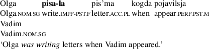
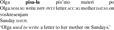
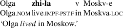
It is a well-attested typological observation that in languages without a distinct morphological progressive form, a morphologically instantiated imperfective aspect inherits the communicative function of the progressive (cf. Bulgarian, Georgian, and Modern Greek; Comrie 1976). This is the basic motivation for treating the progressive as a sub-category of the imperfective. The following examples from Russian demonstrate this distribution: The imperfective form pisa-la in (1) licenses a progressive interpretation, while the same form in (2) refers to a habitual/generic situation; in (3) the same imperfect form zhi-la ‘live’ licenses a continuous non-progressive reading without any overt material.

• (1)

  

• (2)

  

• (3)

  

Languages such as Russian exhibit no ‘explicit’ progressive form since there appears to be no differentiation within the imperfective domain; the imperfective form licenses progressive, habitual/generic and continuous non-progressive interpretations. We label languages that lack a distinct grammatical progressive form as Zero Progressive (ZP) systems.

1.3 Languages with optional progressive morphology

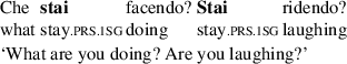
In contrast to languages without a progressive form, in languages which do express non-obligatory progressive morphology, the progressive form serves to stress progressive reading (cf. Spanish, Dutch, and varieties of German). Consider the following examples from Italian (Williams 2002):

• (4)

  

• (5)

  

Example (4) illustrates the use of an optional progressive form within the postural verb construction (verb stare ‘to stay’), while (5) is a present tense sentence in the imperfective aspect without any additional progressive form. Both (4) and (5) license a progressive interpretation. Italian-like languages with an optional progressive form will in the following be labeled as Optional Progressive (OP) systems.

1.4 Languages with a categorical progressive form

In contrast to languages without or optional progressive morphology, there are languages where (i) a progressive form has to be used obligatorily, and (ii) the existence of the progressive blocks the use of the more general form licensing an imperfective interpretation (cf. Swahili, Irish and Hindi). In English, the progressive construction be V+ing is obligatory to express progressive meaning and blocks the usage of the more general forms (e.g., present or simple past), which allow solely for non-progressive readings.

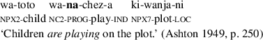
Another exemplary language is Swahili, which has two distinct markers for the imperfective aspect, the non-progressive verbal prefix marker hu- and the progressive marker -na (cf. Ashton 1949; Polomé 1967; Londfors 2003).¹ Both markers are in complimentary distribution where -na calls only for a progressive reading and rules out a non-progressive or habitual/generic reading (cf. (6)). Hu works exactly the other way around: As depicted in examples (7) to (8) this marker licenses only habitual/generic and non-progressive readings.

• (6)

  

• (7)

  

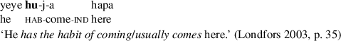
• (8)

  

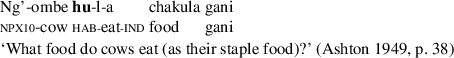
English- and Swahili-like languages with a categorical progressive form will be labeled as Categorical Progressive (CP) systems.

1.5 The progressive-to-imperfective shift

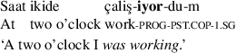
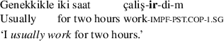
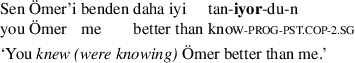
Another observation from cross-linguistic studies is a generalization process of progressive markers: forms once restricted to a progressive reading semantically generalize to license readings of the whole imperfective domain, i.e. even non-progressive and habitual readings (Comrie 1976; Dahl 1985). This generalization has been made on the basis of data from, e.g., Turkish (Göksel and Kerslake 2015, p. 331), as shown in (9) to (12).

• (9)

  

• (10)

  

• (11)

  

• (12)

  

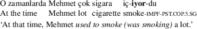
Note that the verb form with -(I)yor in (9) refers to an ongoing event, while the inflected verb with -ir in (10) refers to a habitual reading. Recently, the progressive marker -(I)yor has begun to license a wider range of readings, notably in everyday language. The maker -(I)yor in Modern Turkish occurs with the stative verb ‘to know’, cf. (11), and it is also interchangeably used with the habitual reading, cf. (12). Furthermore, the former imperfective non-progressive marker -ir became unproductive on its path to Modern Turkish and is mostly regarded as archaic. These data indicate that the progressive form of Turkish has expanded to cover the whole imperfective domain by replacing the former non-progressive marker, and thus exemplify the progressive-to-imperfective shift (Bybee et al. 1994). The generalization of the progressive form leads to a system that does not make an explicit distinction for the progressive within the imperfective domain, which results in a ZP language system. We label a language with a ZP system that emerged evidently from a CP system as ZP^∗. Other ZP^∗ languages include e.g. Welsh and Yoruba (Comrie 1976).

1.6 The progressive cycle

Table 1 shows the different systems and languages representing these systems. Note that there are three ‘different’ systems in total, since the fourth system, ZP^∗, conforms to the first system ZP in its systematization; as already mentioned, both systems only differ with regard to their histories: the evidence or non-evidence for a former CP stage. The three systems can intuitively be regarded as distinct strategies for communicating phenomenal (facts of local import, pertaining to specific times) and structural (stable facts that characterize the world as a whole) sub-meanings within the imperfective domain (cf. Goldsmith and Woisetschlaeger 1982). Here, the phenomenal sub-meanings embrace progressive readings, whereas the structural sub-meanings embrace habitual and non-progressive readings. In systems with two forms (OP and CP), the choice of form helps the hearer to correctly identify the speaker’s intended sub-meaning. The ZP/ZP^∗ system uses a single form, relying on the hearer’s understanding of contextual cues for successful communication.

Table 1 The historical progressive cycle and sample languages

The history of English reveals a diachronic process of changes, starting from a ZP system (Middle English) via an OP system (Early Modern English) to a CP system (Present-Day English). Additionally, in comparison to other CP systems (Irish or Swahili), the English progressive marker tends to be more extended inside the imperfective domain (Comrie 1976, p. 38), which indicates that it might generalize over the whole imperfective domain. In other words, English might be in a phase of undergoing a progressive-to-imperfective shift, and is therefore expected to approximate a ZP^∗ system (cf. Table 1). In that particular prospective case English would have accomplished one whole rotation of the progressive cycle.

This progressive cycle is depicted in Fig. 2 as a path from ZP to ZP^∗. We follow Deo’s 2015 characterization, which in turn follows Bybee et al. (1994, Ch. 5). It is assumed that all languages’ imperfective systems can only change in left-to-right direction of this path: Taking a ZP state as point of departure, the grammaticalization of lexical material can lead to the innovation of a grammatical progressive form that is optionally applicable to the former form for the whole domain (OP system). Then, categorization by means of semantic blocking leads to a constrained usage of the former exponent solely for non-progressive readings and obligatory usage of the progressive form (CP system). From there, generalization of the progressive marker leads to the suppression of the former form in the imperfective domain, resulting in a ZP system again. An almost complete rotation is documented for English, and other languages reveal left-to-right movements on parts of that cyclic path, as delineated in the section above. E.g., Modern German is assumed to be in the phase of moving from a ZP to a OP system, while Turkish is about to complete a shift from CP to ZP^∗.

Fig. 2

The progressive path constitutes a full cycle by beginning with ZP and ending with ZP^∗, since both systems are functionally the same; they only differ in terms of the forms that are used. By contrast, the habitual path does not accomplish the full cycle, since there is no evidence for the transition from CH to ZH^∗, in other words: there is no evidence for a generalization of habitual forms within the imperfective domain

It is also important to note that there might be another process of innovation inside the imperfective domain: the emergence of a habitual marker, such as ‘used to’ in English. Again, the initial point is a system without a distinct marker within the imperfective domain (Zero Habitual, ZH). Note that ZH and ZP are identical systems, since both do not make any distinction inside the imperfective domain (cf. Fig. 2). Then, grammaticalization processes might lead to an optional habitual marker (cf. English ‘used to’). This would be an Optional Habitual (OH) state. By drawing parallels with the progressive path the next state would have a categorical habitual marker, a Categorical Habitual (CH) state. And if this categorical habitual marker were to generalize over the domain, the system would end up in a ZH^∗ state, having accomplished the full cycle. So far, data from languages of the world reveal the existence of the progressive cycle, but not of the habitual cycle, since there is no evidence for a CH → ZH^∗ shift, thus there is no generalization of a habitual marker over the whole imperfective domain. The habitual path with the missing CH → ZH^∗ link is also shown in Fig. 2.

Concerning the systematization of the progressive, most of the languages we analyzed can be assigned to one of the three systems: ZP, OP and CP. Empirical data let us suggest that of all languages of the world i) many languages have a system expressed by one of the three states, and ii) comparatively few languages are on a transitional phase depicting a left-to-right shift from one state to the other. This data situation reflects the dynamics of an evolutionary system, where replicators i) most of the time constitute a stable state inside a particular ecological niche, and ii) make fast² shifts from one state to another, driven by environmental influences. In the spirit of applying evolution theory to language change (cf. Jäger 2004; Rosenbach 2008), the evolutionary replicators are here understood as grammatical systems (which are permanently replicated/reproduced by its language users) within the ecological niche ‘imperfective domain’, and the environmental influences which drive them from one state to the other are processes of grammaticalization, involving innovation, categorization and generalization.

Inspired by the work by Jäger (2007, 2014) and especially Deo (2015) we developed an evolutionary population model to capture the evolutionary nature of language change. This model involves a game-theoretic formalization of communication by means of grammatical strategies inside the imperfective domain: the Imperfective Game. In Sect. 2 we introduce the basic notions of game-theoretic modeling and the definition of the Imperfective Game. In Sect. 3 we present the evolutionary population model; and in Sect. 4 we demonstrate its application in synthetic experiments, which we conducted to reconstruct the progressive cycle. We conclude our study in Sect. 5.

2 The Imperfective Game

In the previous section we presented the phenomenon under investigation: the historical progressive cycle. The directed and cyclic property of this phenomenon is assumed to be a result of universal (culture independent) forces, which can be described on the basis of mostly functional factors, such as communicative success and speaker/hearer economy. To get a better insight into the nature of the forces propelling the historical cycle, we present a dynamic model that (i) formalizes the communicative behavior between speaker and hearer as communication strategies, (ii) integrates an iterated learning model for guiding repeated communication, and (iii) simulates an evolutionary path of communication strategies.

The description of the learning model and the evolutionary process is part of the Evolutionary Population Model, which is defined in Sect. 3. In this section we introduce the communication model that determines the range of communicative behavior of speaker and hearer.

The basic communication model is the signaling game (Lewis 1969), a game-theoretic model that formalizes the communicative behavior between speaker and hearer in terms of decoding/encoding patterns between meanings and forms. To formalize communicative behavior that applies to the differentiation between progressive and non-progressive readings, we make use of the vanilla model of Deo’s (2015) Imperfective Game, which is a basic signaling game extended by a contextual space. After introducing this model in Sect. 2.1, we will show in Sect. 2.2 that i) it is possible to describe the typological systems presented in Fig. 2 as communication strategies, and ii) these systems cover only a small subset of all possible communication strategies determined by the Imperfective Game. Finally, in Sect. 2.3 we compare our approach of embedding the Imperfective Game into an Evolutionary Model with Deo’s approach and highlight the advantages of ours.

2.1 Deo’s Vanilla model

As discussed in Sect. 1.6, the imperfective domain can be distributed in two essential sub-domains, namely phenomenal and structural meanings. Furthermore, a progressive form basically expresses a phenomenal meaning, and a habitual form a structural meaning. This distinction is the basic meaning differentiation of the Imperfective Game: the game has a set of two meanings, and a set of two forms respectively. More specifically, the game contains a set of meanings $M = \{m_{p}, m_{s}\}$, containing a phenomenal meaning $m_{p}$ and a structural meaning $m_{s}$; and a set of two forms $F = \{f_{old},f_{new}\}$. Note that according to the progressive cycle there is a state where only one form expresses the whole imperfective domain and, conceivably, through the processes of grammaticalization a second form emerges that expresses a phenomenal reading: the progressive form. To abstract from what kinds of function each form can adopt, the forms are labeled solely according to their historical appearance: $f_{new}$ as grammatical form emerged at a later point in time than $f_{old}$.³

The Imperfective Game is an extended signaling game, since it has an additional set of contexts C. Note that languages that do not explicitly mark a phenomenal reading by a progressive form – hence, languages that do not have a progressive form, such as Russian – need to access contextual cues for prompting a phenomenal reading.⁴ Therefore, the set of contexts contains a contextual cue that is more likely to license a phenomenal reading $c_{p}$ and one that is more likely to license a structural reading $c_{s}$, thus $C = \{c_{p}, c_{s}\}$. Importantly, there is a relationship between the sets C and M in the following way: the contextual cue $c_{s}$ is more likely to license meaning $m_{s}$ and the contextual cue $c_{p}$ is more likely to license meaning $m_{p}$. This relationship is expressed by a modified prior probability function $P \in (\Delta(M))^{C}$, that defines context-dependent probabilities over meanings, as defined in (13). This probability says, for example, that the probability of a phenomenal meaning $m_{p}$ being part of the conversation is 0.9 if contextual cue $c_{p}$ is given, and 0.1 if contextual cue $c_{s}$ is given. Furthermore, the Imperfective Game has a second prior probability function $P_{C} \in \Delta(C)$ that defines prior probabilities over contextual cues. In Deo’s version of the Imperfective Game both contextual cues are assumed to be equiprobable, as defined in (14).

• (13) $P(m_{i}|c_{j}) = \left\{ \begin{array}{cl} 0.9 & \text{if } i = j \\ 0.1 & \text{else} \end{array} \right.$

• (14) $P_{C}(c_{p}) = P_{C}(c_{s}) = 0.5\phantom{\left\{ \begin{array}{cl} 0.9 & \text{if } i = j \\ 0.1 & \text{else} \end{array} \right.}$

The communicative behavior of speaker and hearer are defined as speaker strategy and hearer strategy, appropriately. Both strategy types can be defined as context-unrelated or context-related. Let us first take a look at the more general context-unrelated strategies (note that the context-related strategies will be defined in Sect. 2.2). A speaker strategy s∈S is defined as a function from meaning to form: S:M→F, a hearer strategy h∈H as a function from form to meaning: H:F→M.

For a given meaning m, the communicative success of a strategy pair S,H can then measured by the δ-function: $\delta_{m}(S,H) = 1$, iff H(S(m))=m, else 0. In other words, communication is successful if the hearer construes the meaning the speaker wants to communicate. The utility of the speaker and the hearer each depends on communicative success. The hearer’s utility function $U_{h}$ corresponds to the δ-function and is defined in (15).

• (15) $U_{h}(t,S,H) = \delta_{t}(S,H)$

The speaker’s utility function contains a cost value for the number β of different forms that she has to access. It is given in (16).

• (16) $U_{s}(t,S,H) = \delta_{t}(S,H) - \alpha \times (\beta -1)$

  whereby α is a parameter that determines how highly the speaker values

  costs for multiple forms (β) over communicative success

All in all, the Imperfective Game is defined in (17).

• (17) ${IG} = \langle (S,H), C, M, F, P, P_{C}, U \rangle$ is the Imperfective Game, whereby

  • S and H are speaker and hearer strategies respectively,

  • $C = \{c_{p}, c_{s} \}$ is the set of contextual cues,

  • $M = \{m_{p},m_{s} \}$ is the set of meanings,

  • $F = \{f_{old}, f_{new} \}$ is the set of forms,

  • $P \in (\Delta(M))^{C}$ with $P(m_{i}|c_{j}) = \left\{ \begin{array}{cl} 0.9 & \text{if } i = j \\ 0.1 & \text{else} \end{array} \right.$ is the context-dependent prior probability function over the meaning space,

  • $P_{C} \in \Delta(C)$ with $P_{C}(c_{p}) = P_{C}(c_{s}) = 0.5$ is the contextual cue probability function,

  • $U_{s}$ and $U_{h}$ are the utility functions of speaker and hearer as defined in (16) and (15) respectively.

2.2 Strategy space of the Imperfective Game

The context-related speaker and hearer strategies of the Imperfective Game have to take into account, in addition to form and meaning, the contextual cues of the communicative situation, since they might influence the players’ behavior. Therefore, a context-related speaker strategy $s \in \mathcal{S}$ is defined as a function from context-meaning pairs to forms: $\mathcal{S}: M \times C \rightarrow F$. Similarly, a context-related hearer strategy $h \in \mathcal{H}$ is defined as a function from context-form pairs to meanings: $\mathcal{H}: F \times C \rightarrow M$.⁵ The resulting set of context-related speaker strategies $\mathcal{S}$ and hearer strategies ℋ each contains 16 strategies, delineated in Table 2. Note that four speaker strategies and three hearer strategies are part of the progressive cycle, shaded with a gray background. Additionally, only specific pairs of these strategies are part of the progressive cycle (cf. Table 3):

• 1. The ZP state is represented by the strategy pair $\langle s_{0}, h_{3} \rangle$: the speaker uses the only accessible form for the imperfective domain in her grammar, namely $f_{old}$, represented by the strategy $s_{0}$, and the hearer – without having access to a grammaticalized disambiguating form – only disambiguates via contextual cues, namely he construes $m_{p}$ when $c_{p}$ is given and $m_{s}$ when $c_{s}$ is given, represented by the strategy $h_{3}$.

• 2. The OP state is represented by the strategy pair $\langle s_{2}, h_{1} \rangle$: in the strategy $s_{2}$ the speaker uses the old form $f_{old}$ to express the structural meaning $m_{s}$. To express the phenomenal meaning $m_{p}$ the speaker can use $f_{old}$ or the new form $f_{new}$. In other words, optionality represents the fact that the speaker has two options to express $m_{p}$. Note furthermore, that the new form $f_{new}$ is used to stress a phenomenal reading in the case where the contextual cue $c_{s}$ more likely licenses a structural reading.⁶ Furthermore, the the strategy $h_{1}$ still disambiguates message $f_{old}$ via contextual cues, but message $f_{new}$ is only interpreted as phenomenal meaning $m_{p}$.⁷

• 3. The CP state is represented by the strategy pair $\langle s_{10}, h_{5} \rangle$: the speaker uses a one-to-one mapping between form and meaning: $f_{old}$ to express $m_{s}$ and $f_{new}$ to express $m_{p}$, represented by the strategy $s_{10}$. Likewise, the hearer uses a one-to-one mapping between meaning and form: $f_{old}$ is construed with $m_{s}$ and $f_{new}$ is construed with $m_{p}$, represented by the strategy $h_{5}$. Note that exactly those one-to-one mappings permit to ignore any contextual cues.

• 4. The ZP^∗ state is represented by the strategy pair $\langle s_{15}, h_{3} \rangle$: the speaker’s usage of the new form $f_{new}$ is extended over the whole imperfective domain, represented by the strategy $s_{15}$. As for the ZP state, the hearer can only disambiguates via contextual cues, represented by the strategy $h_{3}$.

Table 2 The set of context-related speaker strategies $\mathcal{S}$ (left table) and the set of context-related hearer strategies ℋ (right table) of the Imperfective Game each contains 16 strategies. Note: the strategies of the progressive cycle are shaded with a gray background, the strategy labels of the habitual path are displayed in boxes

Table 3 The progressive cycle with appropriate strategy pairs

Likewise, the alternative habitual path can be characterized by its possible stages, assuming that it equally would constitute a cycle (cf. Table 4).

• 1. The ZH state is in accordance with the ZP state represented by the strategy pair $\langle s_{0}, h_{3} \rangle$, since the initial state is the one with only one, i.e., the old form $f_{old}$, for the whole imperfective domain.

• 2. The OH state is represented by the strategy pair $\langle s_{4}, h_{11} \rangle$: in the strategy $s_{4}$ the speaker uses the old form $f_{old}$ for the phenomenal meaning $m_{p}$. To express the structural meaning $m_{s}$ the speaker can use $f_{old}$ or the new form $f_{new}$. In other words, optionality represents the fact that the speaker has two options to express $m_{s}$. Note furthermore, that the new form $f_{new}$ is used to stress a structural reading where the contextual cue $c_{p}$ is likely to license a phenomenal reading. Furthermore, the the hearer strategy $h_{11}$ still disambiguates form $f_{old}$ via contextual cues, but the form $f_{new}$ is only interpreted as structural/habitual meaning.

• 3. The CH state is represented by the strategy pair $\langle s_{5}, h_{10} \rangle$: the speaker uses a one-to-one mapping between form and meaning: $f_{old}$ to express $m_{p}$ and $f_{new}$ to express $m_{s}$, exactly the opposite of what happens for the CP state, represented by the strategy $s_{5}$. Likewise, the hearer uses a one-to-one mapping between meaning and form: $f_{old}$ is construed with $m_{p}$ and $f_{new}$ is construed with $m_{s}$, represented by the strategy $h_{10}$. As before, exactly those one-to-one mappings permit to ignore any contextual cues.

• 4. The ZH^∗ state is again in accordance with the ZP^∗ state represented by the strategy pair $\langle s_{15}, h_{3} \rangle$, since the final state only applies one form, namely the new form $f_{new}$, for the whole imperfective domain.

Table 4 The hypothetical habitual cycle with appropriate strategy pairs

2.3 Differences between Deo’s and our model

Our model differs from Deo’s in two major respects, namely, (i) in the parametrization of the Vanilla model itself and (ii) in the usage of the model.

Concerning the definition of the Vanilla model itself: although we adopt Deo’s Vanilla model, we changed one aspect to make it more realistic: the prior probabilities $P_{C}(c)$ of the contextual cues. Note that according to Definition (14) of the original model both contexts are equiprobable, have probability 0.5 each. This is an assumption unsupported empirically, as explained in what follows.

It is reasonable to assume that the value for the context probability supporting a phenomenal meaning can be approximated by the frequency of usage of progressive forms in a language with a categorical progressive system. Furthermore, such usage frequencies can be empirically obtained by corpus studies. We decided to use results from studies using corpora of Modern English texts, since i) English has a categorical progressive, and ii) the level of documentation is higher for English than for any other language. Here, a number of corpus studies showed the relative frequency of progressive forms in written English is between 3% and 4% (cf. Smith 2002). A more recent study analyzed the usage of progressive forms in Corpora of spoken English and came to the result that the usage is slightly higher, namely around 5% (Aarts et al. 2010).

Since spoken English is more representative for our model, we decided to use this value for the approximation for the context probabilities: taking in account the usage of progressive forms in spoken English we assume the value 0.05 for the prior probability of the contextual cue for phenomenal meaning $P_{C}(c_{p})$ and accordingly 0.95 for the $P_{C}(c_{s})$, as given in Definition (15).

• (15) $P_{C}(c_{p}) = 0.05, \hspace{.1cm} P_{C}(c_{s}) = 0.95$

The second aspect relates to the usage of the Vanilla model. First of all a very important difference in our approach is that it explores the full logical strategic space of the Imperfective Game, as depicted in Table 2. Note that Deo exclusively considers the four speaker and three hearer strategies that appear in the progressive cycle (the ones of Table 2 shaded with a grey background) in her analysis. She mentions the importance of considering the whole logical space in footnote 21 (Deo 2015, p. 32):

The strategies considered in this game model do not exhaust the logical space of strategies for the Imperfective Game. For instance, we do not consider strategies in which the state struc is disambiguated (whether in less probable or in all contexts) using a distinct form, say gen either in conjunction with prog alone, impf alone, or both. A more complete game-theoretic account of changes in the imperfective domain must consider these strategic options. I do not consider these here because of the focus on the progressive ≫ imperfective cycling path and the non-attestation of the reverse path (Sect. 4.3).

Note that in our study we explore the full logical space in that we do not restrict the model only to four strategies. The goal of our study is to find a minimal set of assumptions for which our model produces solely the four strategy pairs corresponding to the progressive cycle (out of the 16 × 16 = 256 possibilities), and transitions from one to the other in the expected order. This is different from Deo’s objective, which is to consider only the relevant four strategy pairs and to find explanations for transitions from one to the other.

Another very important difference is the type of evolutionary population model used. Deo uses classical evolutionary game theory (Taylor and Jonker 1978): the replicator-mutator dynamics (cf. Page and Nowak 2002). This approach is a population-based one. It solely considers changes of strategy frequencies in a population of interacting agents; thereby it abstracts from the implementation of single agents. On the contrary, our approach is an agent-based one, where we implement single agents that interact via the Progressive game and update their behavior via the learning rule reinforcement learning (Roth and Erev 1995). Note first of all that it has been shown for a number of games that both approaches, replicator dynamics and reinforcement learning, converge to the same attraction states, thus both dynamics approximate in the long run (cf. Börgers and Sarin 1997).⁸ But our approach has one advantage: it allows us to model in a more detailed way the features of single agents, and this fact plays an important role in the additional assumptions we will add the evolutionary population model, such as childhood asymmetry (cf. Sect. 4.4).

As a further note: since our approach is more detailed on the agent level, one might assume that we use a much more complex model with much more assumptions than Deo does. But the comparison of the models shows otherwise. Deo makes a great number of assumptions for her mutation probabilities. First of all she defines a particular configuration of the 16 values of her mutation matrix $Q''$ based on a number of different hypotheses (Deo 2015, page 41), and then she adds an additional assumption that a specific mutation rate changes with the usage of a variant (Deo 2015, page 41). For example, Yanovich (unpublished) shows that to reconstruct the progressive cycle Deo’s model crucially depends on this particular configuration of the mutation matrix, and it is not very robust for alternating parameters or additional assumptions. In comparison, we stick to a simple evolutionary model with a very simple learning mechanisms, where we add a minimal number of additional assumptions that reproduce the cycle.

2.4 Research question

As we discussed in Sect. 1.6, there is a number of languages that have an optional habitual form, but there is no evidence for the generalization of a habitual marker over the whole imperfective domain. In other words: there is no evidence for a diachronic process leading from state CH to ZH^∗. So the expected diachronic processes are depicted in Fig. 3: the progressive path constitutes a full cycle from state ZP to state ZP^∗, since both systems are functionally the same, they differ solely in the used form $f_{old}$ and $f_{new}$, respectively. In other words, the cycle ends with the same system that it began with, by having replaced $f_{old}$ with $f_{new}$. On the contrary, the habitual path – according to typological data – does not accomplish the full cycle.

Fig. 3

The progressive path constitutes a full cycle by beginning with ZP and ending with ZP^∗: since both systems are functionally the same, differ solely in the used form/exponent. On the contrary, the habitual path does not accomplish the full cycle, since there is no evidence for the transition from CH to ZH^∗. Note that each state is indicated by the strategy pair of the Imperfective Game

Note that while the space of possible strategy pairs is 16 × 16 = 256 in total, we observe only four of them in languages of the world ($\frac{1}{64} \approx 1.6\%$ of all possible strategy pairs). Therefore, our research question deals with the search for explanations for why there is only evidence for the existence of exactly these strategy pairs and exactly in the given order of the progressive/habitual paths, and no evidence for possible other strategy pairs and/or paths. Here, we are particularly interested in analyzing why does the progressive path constitute a cycle, while the habitual path does not.

This research question is examined by a computational synthetic approach: the given game-theoretic model will be embedded into an evolutionary population model, which enables us to simulate language change. We then can analyze under what kind of additional assumptions the expected paths (cf. Fig. 3) can be reconstructed best. In the following section we will introduce the evolutionary population model.

3 Evolutionary population model

A communication system like human language works because it is used in a community all members of which know the conventions and rules on how to use it. Thus, the language community is an essential aspect in understanding the functional aspect of communication. One might ask why language changes at all? If the current system works, since all members know the conventions and rules, there is no need to change, and there is no pressure to force changes. Furthermore, language change is in general not a desired and conscious act. For example, there has not been a person who once proclaimed a need for an additional marker for phenomenal situations in the English language. It just happened somehow.

The source of language change is assumed to be unfaithful reproduction, either in i) repeated communicative acts or ii) first language acquisition/learning. (Computational) models that analyze language change as a result of unfaithful repeated interaction concentrate on so-called horizontal transmission: the way linguistic tokens are exchanged, change and spread in a community, and how they change the linguistic types of its members (cf. Nettle 1999; Ke et al. 2008; Fagyal et al. 2010; Mühlenbernd 2011). Models that analyze language change as a result of unfaithful first language acquisition concentrate on vertical transmission: the way the generational transfer of linguistic tokens shapes the linguistic types of the new generation (cf. Kirby and Hurford 1997; Kirby 2005). Our population model integrates both types of transmission.

3.1 General definition

The evolutionary population model that we present in this section includes all three aspects that seem to be important for understanding language change:

• a language community: a population of agents

• horizontal transmission: repeated interaction of agents of the community

• vertical transmission: agents incorporate a learning model and ‘old’ agents are continuously replaced by ‘new born’ agents

The model can be defined as given in (16).

• (16) EPM = 〈A,SG,LR,m,Λ,θ,κ〉 is an evolutionary population model, whereby

  • $A = \{a_{1}, a_{2} \ldots a_{n} \}$ is a set of n agents,

  • SG is a signaling game,

  • LR is a learning rule,

  • $m \in \mathbb{N}$ is the maximal age of an agent $a_{i} \in A$,

  • Λ is the algorithm that describes the evolutionary process,

  • θ is a start condition of the evolutionary process,

  • κ is the stop condition of the evolutionary process,

  whereby algorithm Λ is given as follows:

  • 1. Set start condition θ

  • 2. Do until stop condition κ is fulfilled:

    for all $a_{i}, a_{j} \in A$:

    • let $a_{i}$ be the speaker S and $a_{j}$ be the hearer H and let them play the signaling game SG

    • update both agents by learning model LR

    • if an agent’s age is above m, replace her by a new agents

Two important aspects of this evolutionary population model are i) the signaling game, and ii) the learning rule. The signaling game in our research is the Imperfective Game as given in (17). The learning rule is a simple learning model, the so-called of Polyá urns reinforcement learning (Bush and Mosteller 1955; Roth and Erev 1995). A number of studies have demonstrated its suitable incorporation within signaling games (cf. Skyrms 1996, 2010). The reinforcement learning account for the given model is described in more detail in Sect. 3.2. All other parameters that must be set for applying the evolutionary population model are discussed in Sect. 4.

3.2 Reinforcement learning model for the Imperfective Game

The reinforcement learning model is implemented as an urn model in the following way. Each agent has four speaker urns $\mho_{S}$ for each context-meaning combination: $\mho_{S}(c_{p},m_{p})$, $\mho_{S}(c_{p},m_{s})$, $\mho_{S}(c_{s},m_{p})$ and $\mho_{S}(c_{s},m_{s})$. Furthermore, each agent has four hearer urns $\mho_{H}$ for each context-form combination: $\mho_{H}(c_{p},f_{old})$, $\mho_{H}(c_{p},f_{new})$, $\mho_{H}(c_{s},f_{old})$ and $\mho_{H}(c_{s},f_{new})$. The speaker urns contain balls of two types corresponding to both forms, either of type $f_{old}$ of of type $f_{new}$. The hearer urns contain balls of two types corresponding to both meanings, either of type $m_{s}$ of of type $m_{p}$.

Now when agents play the Imperfective Game with each other, they make a probabilistic choice of a form (speaker) or meaning (hearer) in dependence on the appropriate urn’s current contents: for a given context c and a given meaning m the speaker draws a ball of type f from urn $\mho_{S}(c,m)$. Afterwards the hearer draws a ball $m'$ from urn $\mho_{H}(c,f)$. If $m = m'$ then the game – and therefore the communication – was successful. Afterwards both interlocutors update their urns depending on the outcome. If the game was successful, both interlocutors add an additional ball of the type they used in that interaction to the appropriate urn: the speaker adds a ball of type f to her urn $\mho_{S}(c,m)$, and the hearer adds a ball of type m to his urn $\mho_{H}(c,f)$. If communication fails, the urns are not updated. In this way each urn’s content encodes at any time information about past successes, namely cumulative reward of former interactions.

As we will explain in Sect. 4.2 there are situations for which neither interlocutor knows the contextual cue. Here the speaker only knows the meaning m she wants to transfer, but there isn’t any contextual cue given. In such a situation the speaker chooses randomly one of two urns, either $\mho_{S}(c_{p},m)$ or $\mho_{S}(c_{s},m)$, and then draws a ball of type f. Afterwards the hearer acts accordingly: he first chooses randomly one of two urns, either $\mho_{H}(c_{p},f)$ or $\mho_{H}(c_{s},f)$, and then draws a ball of type $m'$. Then the urns will be updated as already explained. The idea behind this mechanism is that when no contextual cue is given, both interlocutors are indecisive about contextual support for their decision and act randomly. Note that in the long run each of the two urns will have been chosen the same number of times.

Finally, note that in this model agents (i) play probabilistic strategies, and (ii) do not learn pure strategies as such, but approximate them in the long run. The distance of a probabilistic to a pure strategy can be measured, e.g. by the Hellinger distance (Hellinger 1909). For ease of exposition, we say that an agent ‘uses’ a particular pure strategy, iff it is the Hellinger-closest to her current probabilistic strategy.

4 Synthetic experiments and results

The idea of synthetic experiments to investigate features of linguistic change is inspired by studies in the field of language evolution (cf. Cangelosi and Parisi 1998). The basic idea is as follows: first of all, a computational model is constructed that simulates an evolutionary process of language use according to a specific linguistic feature under investigation. Secondly, particular properties or parameters of the model can be changed, according to specific conjectures. In this way one can test what kind of conjectures are responsible or at least supportive for i) the emergence or ii) the pathway of change of a linguistic feature under investigation by testing which properties simulation the reproduction of an expected evolutionary process.

To analyze possible conjectures responsible for the progressive cycle, we use the synthetic approach in the following way. First of all, we apply a computational model of algorithm Λ as described in (16), whereby the learning rule LR is Pólya urn reinforcement learning and signaling game SG is the Imperfective Game as given in (17) with basic settings α = 0 and $P_{C}(c_{p}) = 0.05$. Secondly, we (i) extend the algorithm by specific properties that are motivated by particular conjectures, and (ii) try to find a minimal set of such additional properties that enable the computational simulation model to reproduce the attested path (Fig. 3). In this way we can test the plausibility that these conjectures are responsible for the emergence of this path and the non-emergence of possible alternative paths in the strategy space of the Imperfective Game (cf. Table 2). The experiments’ parameter settings are given in (17).

• (17) The computational model for our experiments is based on the evolutionary population model EPM = 〈A,SG,LR,m,Λ,θ,κ〉 with the following parameter settings:

  • $A = \{a_{1}, a_{2}, \ldots a_{20} \}$ is a set of 20 agents;

  • Signaling game SG is the Imperfective Game IG as defined in (17) with α = 0 and $P_{C}(c_{p}) = 0.05$;

  • Learning rule LR is implemented as Roth-Erev reinforcement learning (Roth and Erev 1995) as described in Sect. 3.2;

  • Maximal age is m = 4,000 for all agents in A;

  • Λ is the algorithm as given in (16);

  • θ is the following start condition: all agents are assigned with a random age k with 0 ≤ k ≤ m and have an empty learning status (empty urns). For the first 10,000 simulation steps agents can only use form $f_{old}$ to play the Imperfective Game, afterwards the use of $f_{new}$ is introduced;

  • Stop condition κ: no agent has changed her current strategy for the last 40,000 simulation steps⁹ or 1,000,000 simulation steps are reached.

Note that one simulation step entails that every agent $a_{i} \in A$ plays the Imperfective Game one time as a speaker with a randomly chosen agent $a_{j} \in A\setminus\{a_{i}\}$ as a hearer. This implies that every agent is able to interact with every other agent: the population structure resembles a complete network.

4.1 Experiment I: the Vanilla model

100 simulation runs were conducted for the given computational model without additional conjectures. In each run the same population behavior was recorded: while only one form $f_{old}$ is given, all agents immediately learn $s_{0}$ as a speaker strategy and $h_{3}$ as a hearer strategy. Thus, agents manage to learn and use the ZP system: speakers only use one form and hearers use the context information to disambiguate. Since there is only one form given, this behavior was strongly expected. But the behavior after introducing the second form $f_{new}$ was quite unexpected: all agents learn the same hearer strategy $H_{1}$, but fail to agree on a common speaker strategy. There always emerges a mixed population of mainly comprising the strategies $S_{2}$ and $S_{10}$, and also $S_{6}$ and $S_{14}$. Figure 4 shows the fractions of these four speaker strategies after 1,000,000 simulation steps averaged over 100 simulation runs.

Fig. 4

Result of experiment I: initially agents learn the expected ZP strategy $\langle S_{0}, H_{3} \rangle$. After introducing the new form $f_{new}$, all agents learn the same hearer strategy $H_{1}$, but fail to agree on the same speaker strategy: it always emerges a mixed population with almost all agents learning the strategies $S_{2}$, $S_{10}$, $S_{6}$ or $S_{14}$. The percentage values are fractions of the four strategies after 1,000,000 simulation steps averaged over 100 simulation runs

To understand the behavior of the population better, it is helpful to take a closer look at the four strategy pairs, as depicted in Fig. 5: All agents learn the same perfect signaling system when the contextual cue $c_{s}$ is given. But when the contextual cue $c_{p}$ is given all agents learn solely the same hearer strategy – pooling to $m_{p}$, whereas they learn each possible allocation as speaker strategy.¹⁰ Note that the fact that all agents learn the pooling strategy to $m_{p}$ for $c_{p}$ can be explained by the low input of such situation: since $c_{p}$ is solely given with the probability 0.05, agents do not get enough input to learn a signaling system and stick with construing according to the contextual cue $c_{p} \rightarrow m_{p}$.¹¹ And once hearers use a pooling strategy, the speaker strategy is not relevant anymore. Therefore, agents learn any speaker strategy.¹²

Fig. 5

The four different strategy pairs that agents learn in Experiment I, each unraveled to the contextual cues $c_{s}$ (left) and $c_{p}$ (right). For the contextual cue $c_{s}$ all agents learn a perfect signaling system; for the contextual cue $c_{p}$ agents learn the same hearer strategy – pooling to $m_{p}$ – and all possible speaker strategies

4.2 Experiment II: reduced contextual cues

In Experiment I the agents always learn a perfect signaling system when the contextual cue $c_{s}$ is given, but they never learn one when the contextual cue $c_{p}$ is given. Note that in the latter case the hearer always plays the pooling strategy $h_{1}$ for $c_{p}$ and thus always construes any signal with $m_{p}$. In other words: the hearer exclusively construes a signal according to the contextual cue $c_{p}$ and completely ignores the form that is sent. To put it the other way around: the observed behavior is a result of the full exploitation of the contextual cue $c_{p}$.

In the settings of Experiment I the contextual cues are always given. This assumptions is obviously too strong. In many situations there are no contextual cues at all. Therefore, decreasing access to contextual cues will make the model more realistic and pooling strategies such as $h_{1}$ less optimal.

To test this hypothesis, the second Experiment II included 100 simulation runs of the given model plus a reduction of contextual information by 10%. To put it formally: in 90% of all interactions agents play a context-related strategy (cf. Sect. 2.2), and in the remaining 10% of all interactions agents play a context-unrelated strategy (cf. Sect. 2.1).

As the simulation results revealed, this slight reduction of access to contextual cues changed the whole picture: in almost every simulation run the categorical progressive strategy system CP emerged and stabilized. Only in one of 100 simulation runs the categorical habitual strategy CH emerged.¹³ Furthermore, in both cases agents learned the optional systems OP (or OH respectively) on the way, but those systems were always a short intermezzo and never stabilized (cf. Fig. 6).

Fig. 6

Result of Experiment II: agents stabilize on $\langle S_{10}, H_{5} \rangle$ (CP state) in 99% of all simulation runs, and $\langle S_{5}, H_{10} \rangle$ (CH state) in 1%. Both optimal system (OP, OH) are never stabilize (gray: unstable states). Furthermore, strategy pair $\langle S_{15}, H_{3} \rangle$ (ZP^∗/ZH^∗ state) is never reached

This result shows that the reduction of the contextual cue enables the emergence of categorical systems, either CP or CH, with CP much more probable. Note that this is in accordance with empirical data, since there is evidence for a lot of languages to have an explicit progressive marker, but not many languages are known to have an explicit habitual marker (cf. Sect. 1.6).

We assume that the predominance of the emergence of CP in comparison to CH can be explained by the low prior probability of the contextual cue $c_{p}$ (note that $P_{c}(c_{p}) = 0.05$). To test this assumption, we conducted a number of experiments to simulate the behavior of the population for diverse values $0.05 \leq P_{c}(c_{p}) \leq 0.5$. The results confirm our assumption (cf. Fig. 7): the higher the value $P_{c}(c_{p})$, the more probable it is for a CH systems to emerge. This indicates that the empirical evidence for the imbalance between the number languages with a explicit progressive marker and the number of languages with an explicit habitual marker can be explained by the much lower probability of contextual cues for phenomenal situations.

Fig. 7

The percentage of 100 simulation runs resulting in a stable population of users of the categorical progressive system CP or the categorical habitual system CH for different values of the prior probability of the contextual cue $c_{p}$. The results show: by increasing $P_{C}(c_{p})$ the probability for the emergence of the categorical habitual system CH increases (left: table of absolute values, right: graph of percentages over parameter $P_{C}(c_{p})$)

Furthermore, the results of Experiment II and what is considered to be empirically attested for diachronic trajectories in the imperfective domain (Deo 2015) differ in at least two aspects:

• 1. The OP state $\langle S_{2}, H_{1} \rangle$ is only a short intermezzo in the course of the simulation, while in reality it can be maintained for several centuries¹⁴

• 2. The progressive path does not move towards the single-form state $\langle S_{15}, H_{3} \rangle$.

The reason for the first difference is assumed to be as follows: the instability of optional systems may be caused by the fact that we sometimes withdraw the contextual cue: unlike the categorical system, which ignores the cue completely, the optional system crucially relies on it.¹⁵ But even more importantly, optional systems do not constitute a signaling system (Lewis 1969) for both contextual cues, but only for $c_{s}$ (cf. Fig. 5). For contextual cue $c_{p}$, an optional system forms a so-called pooling equilibrium, as depicted in Fig. 8 for the OP system $\langle S_{2}, H_{1} \rangle$. On the other hand, categorical systems form the same signaling system for both contextual cues – as depicted in Fig. 9 for CP system $\langle s_{10}, h_{5} \rangle$ – and therefore they are totally context-independent. In this sense, it is no surprise that the optional systems never stabilize but rather switch directly to the appropriate categorical system. The question is what other property of the real-life imperfective communication makes those systems relatively stable. We leave this point for further research and concentrate on the second aspect: under what circumstances might a perfect context-independent signaling system like CP change towards the single-form system ZP^∗, represented by strategy pair $\langle S_{15}, H_{3} \rangle$?

Fig. 8

The two strategy pairs of the OP system $\langle s_{2}, h_{1} \rangle$: only for contextual cue $c_{s}$ does the strategy pair form a signaling system, whereas for contextual cue $c_{p}$ it forms a so-called pooling equilibrium

Fig. 9

The two strategy pairs of the CP system $\langle s_{10}, h_{5} \rangle$: the strategy pair forms the same signaling system for both contextual cues, is therefore context independent as well as evolutionary stable

4.3 Experiment III: alternating cost parameter

The reason for not reaching the final single-form system $\langle S_{15}, H_{3} \rangle$, as seen in the former experiments, is as follows: a two-form categorical system such CP is i) perfectly efficient, ii) always achieving communicative success, and iii) completely independent of contextual cues. Furthermore, it forms a signaling system (Lewis 1969), and signaling systems have been shown to be evolutionary stable under evolutionary dynamics (Wärneryd 1993). Why would a stable and efficient two-form system such as CP then be replaced by a less efficient single-form system, such as ZP^∗? Intuitively, this would only happen if maintaining the efficient two-form system somehow becomes burdensome.

The shift from a two-form to a one-form system can happen if maintaining a two-form system is more expensive than maintaining a one-form system. Note that the impact of costs for the usage of additional forms in a grammatical system of the given model can be controlled by the α-parameter as given in Definition (16) for the speaker utility. It is a reasonable assumption that if the α-parameter is too high than a one-form system becomes more attractive than a two-form system.¹⁶ Here we make the assumption that this α-parameter randomly changes over time between 0 and 1. Once the α-parameter has exceeded a particular threshold it is expected that the one-form system becomes more attractive and the population will switch to it.

Therefore, in Experiment III, we augmented the model of Experiment II with a randomly changing α-parameter in the range between 0 and 1, each simulation step updates by +0.001 or −0.001. The results were as follows. As in Experiment II, the population first stabilized on a categorical system, and at one point the α-parameter reached a magnitude that favored the usage of a one-form system. But the population never agreed on one particular one-form system, but became a mixed population of ZP and ZP^∗ users, as depicted in Fig. 10.

Fig. 10

Left: Experiment III: The population switches finally to a one-message system, either $\langle S_{0},H_{3} \rangle$ or $\langle S_{15},H_{3} \rangle$, each equiprobable for both paths

All in all, in Experiment III, all runs end up in a mixed population of one-form users, whereby either $f_{old}$ or $f_{new}$ is used. But to achieve the expected picture of the attested paths (Fig. 3), we would expect that $f_{new}$ always generalizes on the progressive path, but never generalizes on the habitual path. In other words, we would expect that a population using strategy pair $\langle S_{10},H_{5} \rangle$ preferably switches to $\langle S_{15},H_{3} \rangle$ eventually, but a population using strategy pair $\langle S_{5},H_{10} \rangle$ does not follow such a switch.

4.4 Experiment IV: childhood asymmetry

What causes the asymmetry of these two paths? Deo (2015) conjectures that it might be due to an asymmetry of input during early language acquisition (Deo 2015, p. 22):

This asymmetry likely stems from the nature of the input to the child, specifically the relative prevalence of PROG forms vs. HAB forms in caregiver speech. [...] this asymmetry in the frequency of phenomenal vs. structural inquiries in child-directed speech would lead to learners generalizing the PROG form rather than any specialized HAB form since exposure to the latter is likely to be less frequent.

Deo refers to a study by Li et al. (2001), who investigated the parental input of progressive vs. non-progressive forms in language acquisition of 2–4 year old children by performing a corpus study using the CHILDES database (MacWhinney 2000). Their study revealed a usage of progressive forms with a frequency of around 63%. Note that this value differs immensely from the frequency for usage of progressive forms in a corpus of spoken English, which was around 5% (cf. Sect. 2.3).

Our model allows us to test Deo’s hypothesis in the following way: we use the frequency values of the corpus study as an indicator for the frequency of contextual cues, as we did it in Sect. 2.3. Furthermore, since agents have an age value defined by their number of interactions, we can define a childhood period by a number of initial interactions $n_{ch} \in \mathbb{N}$. Here we define an agent to be in a childhood period for the initial 10% of her lifetime. Since each agent has a maximal age of m = 4,000 for the current experimental setup, we set $n_{ch} = 400$. Furthermore, we assume that i) each agent as a hearer at age 0 (very early language acquisition) gets a contextual cue with the probability as given from the CHILDES corpus study: $P_{C}(c_{p}) = 0.63$; and ii) that this input decreases linearly during childhood period down to the standard probability: $P_{C}(c_{p}) = 0.05$. Formally, the age-dependent probability for a hearer’s contextual cue $P_{C}: C \times \mathbb{N} \rightarrow [0,1]$ for cue $c_{p}$ at age $n \in \mathbb{N}$ and for cue $c_{s}$ at age $n \in \mathbb{N}$, each is defined in (18).

• (18) $P_{C}(c_{p},n) = \left\{ \begin{array}{c@{\quad}l} ((1-\frac{n}{n_{ch}}) \times 0.58) + 0.05 & \text{if } n \leq n_{ch} \\ 0.05 & \text{otherwise} \end{array} \right., \quad P_{C}(c_{s},n) = 1.0 - P_{C}(c_{p},n)$

Experiment IV involves 100 simulation runs with the same settings as Experiment III plus the changing probability for contextual cues during childhood. The results are depicted in Fig. 11: this childhood input asymmetry leads to the emergence of one form systems for the whole population. Furthermore, for the progressive path, the shift from the categorical progressive system CP to the zero progressive system ZP^∗ emerged twice as often as to the zero progressive system ZP (for CH it was exactly the other way around). In other words: childhood asymmetry supports the asymmetry of the expected trajectories: if the population enters the progressive path, then it generalizes in the most cases (67%) to a new all-purpose imperfective state ZP^∗: here the emerged progressive form $f_{new}$ is eventually the new generalized form. On the other hand, if the population enters the habitual path, the generalization of the habitual marker does not emerge in the majority of simulation runs (note that the habitual path itself emerges only in 1% of all runs, thus is very improbable to emerge from the beginning).¹⁷

Fig. 11

Experiment IV: By assuming that children have more input to phenomenal inquires, agents have a higher input rate of phenomenal meaning $m_{p}$ for the first $n_{ch} = 200$ interactions. The resulting runs support the expected paths: for the habitual path the population switches back to the initial situation in the majority of runs (67%), whereas for the progressive path the population completes the assumed cycle and switches to the final state ZP^∗ $\langle S_{15},H_{3} \rangle$ for 67% of the runs (gray: unstable states)

4.5 Experiment V: alternating population sizes

Experiment IV revealed that we are able to reconstruct the progressive cycle with three additional assumptions that we added to the basic model. But how do alternating population sizes affect the robustness of this result? For our experiments we used a fairly small population size of 20 agents. It is well-known from population dynamics that a small population is more susceptible to drifts from one local optimum to the other than a large population. Therefore we tested the model with the settings of Experiment IV but for different population sizes: 10, 20, 50 and 100. As a basic result it turned out that population size did not have an impact on the course of change. But it had an impact on the duration of transitions between different states.

For each setting (population size 10, 20, 50 and 100) we conducted multiple simulation runs and randomly chose 50 runs for which the progressive cycle was reconstructed.¹⁸ For each setting the population switched directly from a ZP to an OP system after the new form was introduced. But the transition from CP to ZP^∗ took generally a very long time, and – as the data revealed – this duration was strongly influenced by population size: the larger the population size, the longer the transition. Table 5 shows the average number of simulation steps for the transition from CP to ZP^∗ for the different population sizes.

Table 5 Average runtime (in simulation steps, averaged over 50 simulation runs) for the switch from a CP to a ZP^∗ system for different population sizes

All in all, the results suggest that population size does not impact the general observation, namely that the progressive cycle can be reconstructed with the three additional conjectures that we added to the basic model. But one could ask if all three conjectures together are necessary for a successful reconstruction. Do they really build a minimal set of additional conjectures?

4.6 Experiment VI: testing all configurations of additional conjectures

To test if all three conjectures together are necessary to reconstruct the progressive cycle, it is essential to test all possible configurations of including or excluding each conjecture. Table 6 contains all possible eight configurations and the appropriate results, which are delineated in more detailed in what follows.

Table 6 All possible eight configurations of additional conjectures reduction of contextual cues (RCC), alternating costs (ALTC), and childhood asymmetry (CHA). As observable, solely the configuration of all three conjectures together enables to reconstruct the progressive cycle

Configuration 1 corresponds to Experiment I: the Vanilla model without additional conjectures. Note that here the result was the emergence of a mixed population containing the strategies pairs $\langle S_{2},H_{1} \rangle$, $\langle S_{10},H_{1} \rangle$, $\langle S_{6},H_{1} \rangle$ and $\langle S_{14},H_{1} \rangle$. Configuration 2 corresponds to Experiment II: the only additional conjecture is the reduction of contextual cues. Here the strategy $\langle S_{10},H_{5} \rangle$ – the CP system – emerges in 99% of all simulation runs.

Configuration 3 has as the only additional conjecture the alternating cost factor, configuration 4 as the only additional conjecture the childhood asymmetry. But each factor alone does not have any impact on the result, in both cases the result of Experiment I emerges. But as observed in configuration 7, both conjectures together change the picture. Here, too, first the mixed population such as in Experiment I emerges, but eventually the system shifts to a one-form system, either ZP or ZP^∗.

Configuration 5 corresponds to Experiment III. Note that here first the CP system emerges in 99% of all simulation runs, and the population switches to a mixed population of one-form strategies. Configuration 6 has two additional conjectures – the reduction of contextual cues and childhood asymmetry. The result is such as the on of Experiment II: the emergence and maintenance of the CP system. In other words, the childhood asymmetry has no impact here.

As the results reveal, only configuration 8 – the addition of all three conjectures – enables us to reconstruct the progressive cycle. But there are further conclusions that can be made from these results. One is that the reduction of contextual cues is essential for the system to switch to the categorical system CP. Note that only in those configurations (2, 5, 6 and 8) the CP system emerges eventually or as an intermediate step. Furthermore, only the addition of both alternating costs and childhood asymmetry facilitates the final switch to a population-wide one-form system, as observable from the results of configurations 7 and 8 in comparison to the results of all the other configurations. All in all, we can conclude that the reduction of contextual cues is a necessary condition for a categorical system to emerge, and the alternation of costs in combination with childhood asymmetry is a necessary condition for the system to switch back to a one-form system eventually.

5 Conclusion

We presented a computational approach to study a well-attested phenomenon in morpho-semantic change: the progressive cycle. Based on a game-theoretic model by Deo (2015) – the Imperfective Game – we investigated which types of grammars would emerge from first principles in a population of agents exposed to dynamics of evolution and learning. More concretely, we used experiments with reinforcement learning agents playing the Imperfective Game with the full strategy space to investigate whether the empirically observed grammar changes involving the imperfective, progressive and habitual would emerge in this setting. By adding the following three conjectures to the basic model, we managed to reconstruct the emergence of the very frequently occurring progressive cycle in most experiments:

• 1. Withdrawing contextual cues for 10% of all interactions;

• 2. Alternating the cost parameter that defines how highly the speaker values linguistic clarity over signaling costs;

• 3. Higher frequency of contextual cues for phenomenal situations during childhood according to results from corpus studies.

There is a number of points open for discussion. First of all, it is not resolved what kind of conjectures could make both optional systems more stable. Typological data reveal temporally stable OP systems (e.g. Dutch, German, Italian, Spanish) and OH systems (e.g. English, Lithuanian, North Welsh). The given model cannot deliver this. The reason is probably that the modeling of the contextual space is too strict. For instance, instead of having a set of two particular contextual cues, it might be more realistic to have a contextual space, which licenses different readings to a particular degree. And secondly, further conjectures can be tested which by replacing the ones given here might also lead to the expected paths. E.g., instead of assuming alternating costs for the more complex system, it could be assumed that the older form $f_{old}$ might become less attractive over time.

For future research it might be worthwhile to consider the computational models to be fruitfully applied to similar phenomena to the progressive cycle in historical semantics. Grammaticalization phenomena often display a similar diachronic course. For example, in the so-called aoristic drift (Meillet 1909) the ‘present perfect’ invades the domain of the ‘past tense’. Yet another example is the Jespersen Cycle (cf. Dahl 1979): here a marker for ‘emphatic negation’ eventually invades the domain of negation and drives out the former marker. The fact that a very similar diachronic schema – the fight for a grammatical (sub-)domain of two competing variants and the total invasion of the newcomer – emerges in different empirically observed cycles suggests that the factors creating that schema must be either quite general or having similar effects. Evolutionary modeling can help us to understand the relationship of those factors.

By building on previous evolutionary work on the aoristic drift (Schaden 2012) and the Jespersen cycle (cf. Ahern and Clark 2014) we can define computational models which in very general terms capture potentially relevant properties of diachronic phenomena such as the ones we mentioned above. Then we can run those models and see whether they reproduce the historical trajectories that we actually observe. Comparing the output of models incorporating different properties of the cycles, we can find out which properties of competing morphological variants can be responsible for frequent diachronic patterns as seen in phenomena such as the progressive cycle, the aoristic drift, and the Jespersen cycle. We can outline how different stages of the relevant cycles can be modeled as strategies of mapping forms and meanings employed by language-learning agents, how various factors can change the strategies that agents adopt, and how those factors can or cannot reasonably be transferred from on to the other phenomenon of grammaticalization.

References

Aarts, B., Close, J., & Wallis, S. (2010). Recent changes in the use of the progressive construction in English. In B. Cappelle & N. Wada (Eds.), Distinctions in English grammar (pp. 148–167). Tokyo: Kaitakusha.
Ahern, C., & Clark, R. (2014). Diachronic processes in language as signaling under conflicting interests. In E. Cartmill (Ed.), The evolution of language: proceedings of the tenth international conference on the evolution of language (pp. 25–32). Singapore: World Scientific.
Argiento, R., Pemantle, R., Skyrms, B., & Volkov, S. (2009). Learning to signal: analysis of a micro-level Reinforcement model. Stochastic Processes and their Applications, 119, 373–390.
Ashton, E. (1949). Swahili grammar. London: Longman.
Barrett, J. A. (2006). Numerical simulations of the Lewis signaling game: learning strategies, pooling equilibria, and the evolution of grammar. Irvine: University of California. Technical Report MBS 06-09, Institute for Mathematical Behavioral Science.
Bonami, O. (2015). Periphrasis as collocation. Morphology, 25(1), 63–110.
Börgers, T., & Sarin, R. (1997). Learning through reinforcement and replicator dynamics. Journal of Economic Theory, 77(1), 1–14.
Brown, D., Chumakina, M., Corbett, G., Popova, G., & Spencer, A. (2012). Defining ‘periphrasis’: key notions. Morphology, 22(2), 233–275.
Bush, R., & Mosteller, F. (1955). Stochastic models for learning. New York, NY: Wiley.
Bybee, J., Perkins, R., & Pagliuca, W. (1994). The evolution of grammar. Tense, aspect, and modality in the languages of the world. Chicago: Chicago University Press.
Cangelosi, A., & Parisi, D. (1998). The emergence of a ‘language’ in an evolving population of neural networks. Connection Science, 10(2), 83–97.
Comrie, B. (1976). Aspect. Cambridge: Cambridge University Press.
Dahl, Ö. (1979). Typology of sentence negation. Linguistics, 17(1–2), 79–106.
Dahl, Ö. (1985). Tense and aspect systems. Oxford: Blackwell.
Deo, A. (2006). Tense and aspect in Indo-Aryan languages: variation and diachrony. Doctoral dissertation, Stanford University.
Deo, A. (2015). The semantic and pragmatic underpinnings of grammaticalization paths: the progressive to imperfective shift. Semantics and Pragmatics, 8, 1–52, article 14.
Ebert, K. (2000). Progressive markers in the Germanic languages. In O. Dahl (Ed.), Tense and aspect in the languages of Europe (pp. 605–653). Berlin: de Gruyter.
Enke, D., Mühlenbernd, R., & Yanovich, I. (2016). The emergence of the progressive to imperfective diachronic cycle in reinforcement-learning agents. In S. Roberts, C. Cuskley, L. McCrohon, L. Barceló-Coblijn, O. Feher, & T. Verhoef (Eds.), Proceedings of the 11th international conference on the evolution of language (Evolang 11).
Fagyal, Z., Swarup, S., Escobar, A. M., Gasser, L., & Lakkaraju, K. (2010). Centers and peripheries: network roles in language change. Lingua, 120, 2061–2079.
Göksel, A., & Kerslake, C. (2015). Turkish: a comprehensive grammar. London: Routledge.
Goldsmith, J., & Woisetschlaeger, E. (1982). The logic of the English progressive. Linguistic Inquiry, 13(1), 79–89.
Hellinger, E. (1909). Neue Begründung der Theorie quadratischer Formen von unendlichvielen Veränderlichen. Journal für die reine und angewandte Mathematik, 136, 210–271.
Horn, L. (1984). Towards a new taxonomy of pragmatic inference: Q-based and R-based implicature. In D. Schiffrin (Ed.), Meaning, form, and use in context: linguistic applications (pp. 11–42). Washington: Georgetown University Press.
Huttegger, S. M. (2007). Evolution and the explanation of meaning. Philosophy of Science, 74(1), 1–27.
Huttegger, S. M., & Zollman, K. J. S. (2011). Signaling games: dynamics of evolution and learning. In A. Benz, C. Ebert, G. Jäger, & R. van Rooij (Eds.), Language, games, and evolution (pp. 160–176). Berlin: Springer.
Jäger, G. (2004). Evolutionary game theory for linguists (Tech. Rep.). Stanford, University and University of Potsdam.
Jäger, G. (2007). Evolutionary game theory and typology: a case study. Language, 83(1), 74–109.
Jäger, G. (2014). What is a universal? On the explanatory potential of evolutionary game theory in linguistics. In E. McCready, K. Yabushita, & K. Yoshimoto (Eds.), Formal approaches to semantics and pragmatics (pp. 85–103). Dordrecht: Springer.
Ke, J., Gong, T., & Wang, W. S.-Y. (2008). Language change and social networks. Communications in Computational Physics, 3(4), 935–949.
Kirby, S. (2005). The evolution of meaning-space structure through iterated learning. In A. Cangelosi & C. Nehaniv (Eds.), Second international symposium on the emergence and evolution of linguistic communication (pp. 56–63).
Kirby, S., & Hurford, J. (1997). Learning, culture and evolution in the origin of linguistic constraints. In P. Husbands & I. Harvey (Eds.), Proceedings of the fourth European conference on artificial life (pp. 493–502). Cambridge: MIT Press.
Lewis, D. (1969). Convention. Cambridge: Harvard University Press.
Li, P., Maher, S., Newmark, E., & Hurley, J. (2001). The role of parental input in the acquisition of tense-aspect morphology. Journal of Cognitive Science, 2(1), 119–143.
Londfors, A.-L. (2003). Tense and aspect in Swahil. Unpublished manuscript.
MacWhinney, B. (2000). The CHILDES project: tools for analyzing talk. Hillsdale: Erlbaum.
Meillet, A. (1909). Sur la disparition des formes simples du prétérit. In Linguistique historique et linguistique générale (pp. 149–158). Geneve/Paris: Slatkine/Champion.
Mühlenbernd, R. (2011). Learning with neighbours. Synthese, 183(S1), 87–109.
Mühlenbernd, R. (2013). Signals and the structure of societies. Doctoral Thesis, University of Tübingen, TOBIAS-Lib Online Publication.
Nettle, D. (1999). Using social impact theory to simulate language change. Lingua, 108(2–3), 95–117.
Page, K. M., & Nowak, M. A. (2002). Unifying evolutionary dynamics. Journal of theoretical biology, 219(1), 93–98.
Polomé, E. (1967). Swahili language handbook. Washington D.C.: Center for Applied Linguistics.
Rosenbach, A. (2008). Language change as cultural evolution: Evolutionary approaches to language change. In R. Eckardt, G. Jäger, & T. Veenstra (Eds.), Variation, selection, development: probing the evolutionary model of language change (pp. 23–74). Berlin: de Gruyter.
Roth, A. E., & Erev, I. (1995). Learning in extensive-form games: experimental data and simple dynamic models in the intermediate term. Games and Economic Behaviour, 8, 164–212.
Schaden, G. (2012). Modelling the ‘aoristic drift of the present perfect’ as inflation: an essay in historical pragmatics. International Review of Pragmatics, 4, 261–292.
Skyrms, B. (1996). Evolution of the social contract. Cambridge: Cambridge University Press.
Skyrms, B. (2010). Signals: evolution, learning, and information. London: Oxford University Press.
Smith, N. (2002). Ever moving on? The progressive in recent British English. In P. Peters, P. Collins, & A. Smith (Eds.), New frontiers in corpus research (pp. 317–330). Amsterdam: Rodopi.
Taylor, P. D., & Jonker, L. B. (1978). Evolutionary stable strategies and game dynamics. Mathematical Biosciences, 40(1), 145–156.
Wärneryd, K. (1993). Cheap talk, coordination, and evolutionary stability. Games and Economic Behavior, 5, 532–546.
Williams, C. (2002). Non-progressive and progressive aspect in English. Fasano: Schena.
Yanovich, I. (unpublished). Analysing imperfective games. Unpublished manuscript. Eberhard Karls Universität Tübingen.
Author information
Authors and Affiliations
Corresponding author
Additional information
We express our thanks to the audiences of the Tübingen, Munich, and Stanford seminars, of the 17th International Morphology Meeting (Vienna), PLC 40 (Philadelphia), Evolang XI (New Orleans), Germanic Linguistics Roundtable (Berkeley), Diskussionsforum Linguistik (Zurich), and SLE 49 (Naples). Special thanks are owed to Christopher Ahern, Phillip Alday, Sara Sanchez Alonso, Christian Bentz, Heather Burnett, Ashwini Deo, Dieter Gunkel, Olav Hackstein, Gerhard Jäger, Guido Seiler, Thilo Weber, and Igor Yanovich. Any errors that remain are our own responsibility. We gratefully acknowledge the support of the ERC under project EVOLAEMP, http://www.evolaemp.uni-tuebingen.de (RM), the Department of Linguistics at Eberhard Karls University, Tübingen (RM) and the Institute of German Philology of LMU Munich (DE).
Rights and permissions
About this article
Cite this article
Mühlenbernd, R., Enke, D. The grammaticalization cycle of the progressive. Morphology 27, 497–526 (2017). https://doi.org/10.1007/s11525-017-9310-2
Received:
Accepted:
Published:
Issue Date:
DOI: https://doi.org/10.1007/s11525-017-9310-2