
Abstract
In this information age, high data rates and good reliability features are becoming the dominant factors for a successful deployment of commercial networks. Increasing capacity with finite power requirement in wireless networks is one of the main challenges for high speed communications. A new method of power allocation in wireless communication using beamforming vector based sectored relay planning for capacity enhancement has been proposed. It has been observed that any number of terminals (receive antennas) in the downlink can be incorporated without the requirement of additional link budget. Moreover, it has also been observed in the proposed technique that required power is also independent of coverage area i.e., the channel losses at cell borders. This optimal power allocation has been observed using beamforming vector. The beamforming vector becomes independent of transmitter diversity and is the function of receive antennas on both wireless backhaul and access link (sampled impulse response). The target signal-to-interference-noise-ratio (SINR) in the proposed technique can be achieved at small and finite power; therefore any capacity can be achieved at the target SINR. This is in contradiction to the major outcomes of the Shannon’s theorem. The simulations have been carried out in Matlab and the results given in the form of various plots and graphs.
1 Introduction
High capacity in 4G LTE-A cell brusquely the incorporation of multiple antennas at every node of network viz base station (BS), relay node (RN) or user equipment (UE). A linear proportionate relationship exists between the cell throughput and the number of receive or transmit antennas, provided the spatial dimensions and resource blocks are shared as fair as possible, among multiple users, in terms of achieving the high spectral efficiency for LTE-A system as a whole. Allowing many users to communicate in parallel improves the overall spectral efficiency, but the approach will create inter-user-interference at the receiver site, that could degrade the system performance. This necessities for the division of LTE-A networks into different sectors and applying the fixed frequency re-sue pattern in these sectors to reduce interference. The received signal power can be increased by ensuring the data signals are pointing in the desired direction i.e. towards the intended users. This demands a beamforming approach in multi-input–multi-output systems, where a signal is transmitted from multiple antennas using different relative amplitudes and phases such that the constructive adding of signals occurs in the desired directions and vice versa in the undesired direction. Many cooperative multicast methods having trade-off between high through-put and better fairness is the active research area in the given communication. The relay node placement and power allocation in wireless networks is crucial in co-operative environment. By using relay nodes deployment cost is reduced and wide coverage is provided to users, while maintaining better quality of services [1,2,3,4]. Several techniques have been proposed to fully or partially mitigate the inter-user-interference and provide high signaling data rate. In [5] power budget analysis is used to support the signaling data rate The limitation of the paper is that power budget used can be greater than actual power used for user data transfer. If all the terminals (receiving antennas) in the cell are not frequently receiving some information at a given time, there is the limit in the capacity of the wireless networks. In [6] increasing the power at relay node leads to the increase in capacity. Thus the data rate becomes dependent of the required transmit power and the Shannon capacity can become the maximum achievable capacity. Authors in [7] tried to maximize the network capacity while maintaining the minimum installation cost but no proper mathematical analysis for interference management was found in the paper. Network coding done in [8] improves the system throughput effectively, but large time delay limits the performance of system. In [9] decode and forward protocol is investigated, based on two stage co-operation, i.e., at first stage BS transmits data and only users with good channel conditions can decode the data correctly. In second stage all the relays transmit the data to rest of users. This improves the throughput but at the cost of high power consumption.
In this paper, a novel technique is introduced with new concepts, which could support massive MIMO (large number of receive antennas) with small and finite power. The proposed method is based on sectored relay planning (RNs deployed at various sectors of LTE-A cell) and incorporates the use of beamforming vector for capacity enhancement. The proposed beamforming vector not only solves the low SINR problem of cell edge users but also achieves the capacity beyond Shannon limit (Green capacity). The power allocation problem is solved using beamforming vector based sectored relay planning (BFVSRP) algorithm. This allows us to obtain quick approximation of SINR on both backhaul and access links, that are very close to target SINR for achieving the Green capacity.
2 System Model
Consider a tri-sectored LTE-A cell having relay node (RN) deployed at a pre-defined location k (k = 1, 2, 3). At each location the RN is served by a base station (BS) or eNodeB (eNB). The eNB is equipped with Nt ≥ 2 transmit antennas and RN with Nj ≥ 2 antennas. Considering m ∈ M users equipped with Nr ≥ 2 receive antennas, distributed uniformly in the cell and assuming all the users follow Gaussian distribution for sufficiently large numbers of variables (antennas), as per the central limit theorem [10, 11]. Let \(H_{mk} \in {\text{C}}^{{{\text{N}}_{\text{t}} \times {\text{N}}_{\text{j}} }}\) denote the channel between eNB and kth positioned relay for the mth user and \(G_{mk} \in {\text{C}}^{{{\text{N}}_{\text{j}} \times {\text{N}}_{\text{r}} }}\) denote the channel between kth relay and the mth user. The collection of the entire channel vectors (known as channel state information (CSI)) \(\left\{ {H_{jmk} } \right\}_{j,m = 1,k = 1}^{{N_{j,} M,k_{max} }}\) and \(\left\{ {G_{rmk} } \right\}_{r,m = 1,k = 1}^{{N_{r,} M,k_{max} }}\) is assumed to be perfectly known at both transmitters i.e., eNB as well as RNs for backhaul (relay) link and access link respectively [12]. The signal received at kth relay in the first timeslot is given by linear input–output model as follows:
where \(n_{m}\) ∈ C is the combined vector of additive noise and interference from surrounding systems and is modeled as complex Gaussian distributed nm ~ C η \(\left( {0,\sigma^{2} I_{{N_{t} }} } \right)\), σ2 is the noise power. The transmitted signal \(X \in C^{{N_{t} }}_{ }\) contains data symbols intended for mth user via kth relay path using beamforming vector \(v_{mk} \left( {v_{mk} \in C^{{N_{t} }} } \right)\). The beamforming vector \(v_{mk}\) obviates the need of any kind of coordination between the relays and also suppresses inter or multi relay interference while making the system more tractable. The power resources available for transmission need to be constrained to make the system more practical [13]. We assume there are l ∈ L power constraints available for transmitted signal such that,
where \(W_{mk} \epsilon C^{{N_{t} \times N_{t} }}\) is the Hermitian positive semi-definite weighting matrix. Thus Eq. (1) can be rewritten as follows:
Each kth positioned relay linearly processes the received signal using weighting matrix Fmk and transmit Tmk = FmkYmk to the mth user via kth access link, in the second time slot. The aggregate power constraint at kth positioned relay is given by,
Prk is the power at kth positioned relay. The signal received at receiver is processed using Wiener Filtering.
The achievable information rate or mutual information and hence capacity, which is maximum of mutual information in light of information theory [14], over both links (relay as well as access link) for the mth user describes the number of bits that can be conveyed to the user m with an arbitrarily low probability of decoding error and is given as:
where \(SINR_{mk}\) is the signal-to-interference noise ratio expressed by mth user for the kth positioned relay and access link. \(\beta_{1} \in \left\{ {0.5,0.75} \right\}\) and \(\beta_{2} \in \left\{ {1,2} \right\}\), reflect the practical bandwidth and SINR efficiency of LTE channel respectively. The expression for \(SINR_{mk}\) for the Information rate computation over both links is given by:
The user performance function \(I_{mk}\) is measured by an arbitrary continuous, differentiable and strictly monotonically increasing function,\(g_{mk} \left( {SINR_{mk} } \right)\). The function satisfies \(g_{mk} \left( 0 \right) = 0\), for notational convenience. Thus Eq. (5) can be rewritten as:
The vector \(v_{mk}\) for both links only appears in the SINR expression as an inner product with the channels \(H_{jmk} W_{mk}\) and \(G_{rmk} F_{mk} Y_{mk}\) for all the m users, thus any power allocated outside span is wasted and therefore affects the performance, and also the vector \(v_{mk}\) for both the links is the function of receive antennas on both links. The vectors are thus defined as:
3 Optimal Power Allocation Using Beamforming Vector
The transmit beamforming direction \(\bar{v}_{mk}\) for all the m users effect the SINRs of all the co-users \(i\epsilon C_{mk} \backslash \left\{m \right\}\). A heuristic way to balance between signal and interference is to maximize the SINR on both links, which we define as:
for some parameters \(\eta_{mk} \ge 0\). The following heuristic beamforming vectors maximize the SINRs of relay and access link of Eqs. (9), (10) respectively as follows:
where \(I_{{N_{j} }}\) is the identity matrix of receive antennas at kth RN
where \(I_{{ N_{r} }}\) is the identity matrix of receive antennas at UE.
The expressions of Eqs. (11), (12) resemble that of wiener filtering and the beamforming vector \(v_{mk}^{{*\left( {SINR} \right)}}\) become the function of multi-antenna receiver. When the beamforming direction \(\left\{ {\bar{v}_{jmk} } \right\}_{j > 1,m = 1,k = 1}^{{N_{j} M,k_{max} }}\) over relay link and \(\left\{ {\bar{v}_{rmk} } \right\}_{r > 1,m = 1,k = 1}^{{N_{r} M,k_{max} }}\) over access link have been selected, the power allocation \(\left\{ {p_{jmk} } \right\}_{j > 1,m = 1,k = 1}^{{N_{j} M,k_{max} }}\) and \(\left\{ {p_{rmk} } \right\}_{r > 1,m = 1,k = 1}^{{N_{r} M,k_{max} }}\) over relay and access links respectively will ultimately determine the operating point in the performance region that is achieved by a heuristic transmit strategy [15]. The SINR of Eqs. (9), (10) will become,
with fixed \(\rho_{{m_{i} }} \left( m \right) = \left| {H_{{jm_{i} }}^{H} W_{{m_{i} }} \bar{v}_{{jm_{i} }} } \right|^{2}\) for relay link and \(\rho_{{m_{i} }} \left( m \right) = \left| {G_{{rm_{i} }}^{H} F_{{m_{i} }} Y_{{m_{i} }} \bar{v}_{{rm_{i} }} } \right|^{2}\) for access link for all m and mi. The user performance function \(g_{mk}^{ } \left( {I_{mk} } \right)\) on both links is the concave function with invertible derivatives, thus optimal allocation maximizes the information rate \(I_{mk}\) on both links as [16]:
Subject to \(\mathop \sum \limits_{ } p_{jmk} \le P_{b}\) on relay link and
Subject to \(\mathop \sum \limits_{ } p_{rmk} \le P_{rk}\) on access link
Using Langrage’s function to solve the convexity of Eqs. (15), (16) [17], we have
where \(\frac{1}{{v_{j} }}\), \(\frac{1}{{v_{r} }}\) are the Langrage’s multiplier’s associated with relay and access link respectively. Using stationary Karush–Kuhn–Tucker (KKT) condition in Eqs. (17), (18) and replacing all negative values with zero [18], we get,
where \(\frac{d}{dk}g_{mk} \left( x \right) = g_{mk}^{'} \left( x \right)\)
Thus the power allocation on information rate for both links are based on
The resulting power allocation of Eqs. (19), (20) will become
Thus the power allocated on both the links for achieving the maximum information rate is on the basis of some user dependent function \(W_{lmk} > 0\) and \(t_{lmk} > 0\) and zero power is allocated to the users with weakest weights. The column of width of either \(W_{lmk}\) on the relay link or \(t_{lmk}\) on the access link and height \(\frac{{\sigma_{m}^{2} }}{{W_{lmk} }}\) on relay link and \(\frac{{\sigma_{m}^{2} }}{{t_{lmk} }}\) on access link represents each user m. Thus the power allocation result in water filling phenomenon as depicted from our results. Increasing \(W_{lk}\) and \(t_{lk}\) will increase power allocated to user m.
4 Algorithm
The significance of resource allocation is the coupling between users; in terms of inter user interference and power constraints on both links [19]. Thus the beamforming for each user is optimized separately and sequentially. At first
Find \(v_{jmk} ,v_{rmk} , \theta_{mik} ,\mathop {\overbrace {\theta }}\nolimits_{mik} ,P_{b ,} P_{rk } \,\,\,\,\forall m,i i \ne m\)
Subject to
-
1.
\(\frac{{\left| {H_{jmk} W_{jmk} v_{jmk} } \right|^{2} }}{{\sigma_{m}^{2} + \sum\nolimits_{mi \ne m} {\mathop {\overbrace {\theta }}\nolimits_{jmik}^{2} } }} \ge \gamma_{jmk} \,{\text{on}}\,{\text{relay}}\,{\text{link}}\)
where \(\gamma_{jmk}\) is the CDF of SINR experienced by mth user on the relay link
$$\frac{{\left| {G_{rmk} t_{rmk} v_{rmk} } \right|^{2} }}{{\sigma_{m}^{2} + \sum\nolimits_{mi \ne m } {\mathop {\overbrace {\theta }}\nolimits_{rmik}^{2} } }} \ge \gamma_{rmk} \,{\text{on}}\,{\text{access}}\,{\text{link}}$$where \(\gamma_{rmk}\) is the CDF of SINR experienced by mth user on the access link
-
2.
-
3.


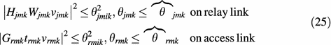
\(\theta_{mik} ,\mathop {\overbrace {\theta }}\nolimits_{mik} ,\) are the non-negative auxiliary variables and are the functions of receive antennas at each node(relay or user equipment). The squared variable \(\theta_{mik}^{2}\) is actually interference generated at mth user, while \(\mathop {\overbrace {\theta }}\nolimits_{mik}^{2}\) is its believed value in beamforming optimization. We denote the Lagrange’s multipliers by \(\lambda_{mk}\) and \(\theta_{mk}\) for interference and power consistency constraints, respectively. Equation (25) can be decomposed into the following convex problems on both relay and access links respectively as [20]:
The master dual problem on both the links is given as [21]:
This decomposition enables an iterative solutions where the sub-problems in Eqs. (26)–(29) are solved for constant values on the Lagrange’s multiplier \(\lambda_{mik} \forall mi \ne m\) and \(\theta_{mk} \forall m.\) The Lagrange’s multipliers can be viewed as prices for causing interference and for consuming transmit power, and these prices are iteratively adjusted by master problem of Eqs. (28), (29), until convergence. The convex problem of Eqs. (26), (27) enables an iterative procedure for achieving Lagrange’s multipliers in (n + 1)th iteration as follows [22]:
where \(\xi > 0\) is the step size.
The Eqs. (30), (32) require exchange of Lagrange’s multipliers \(\lambda_{mik}^{\left( n \right)}\) completed in the nth iteration between the base station and the kth relay node on the backhaul link and between kth relay node and user equipment on the access link. Similarly, the Eqs. (31), (33) require exchange of power constraint coefficients between base station and the kth relay node on the backhaul link and between kth relay node and user equipment on the access link [23].
4.1 Beamforming Vector Based Sectored Relay Planning Algorithm (Bfvsrp)
The proposed BFVSRP is explained briefly in steps as:
Step 1 Input
Step size \(\xi > 0\)(fixed or adaptive)
k = 1 (Intialiaziation)
kmax = 3 (Total sectors of cell)
Pb (Power at eNB.)
Prk (Power at kth relay node.)
\(g_{m} \left( {SINR_{m} } \right) \ge r_{m}^{*}\) for each user m.
\({\text{Initialization }}\) of \(\lambda_{\text{jmik}}^{(1)} ,\lambda_{\text{rmik}}^{(1)} ,\theta_{\text{jmk}}^{(1)} ,\theta_{\text{rmk}}^{(1)}\) (equal to zero)
Step 2 Processing
-
1.
Shannon direct link capacity
Calculate the channel capacity (Shannon capacity) of direct link modeled by MIMO antennas as:
$$C = log \left[det\left( {I_{{N_{r} }} + \frac{\gamma }{{N_{t} }}{\mathcal{H}\mathcal{H}^{\prime}}} \right) \right]$$\({\mathcal{H}}\) is the \(N_{r} \times N_{t}\) channel matrix
-
2.
Sectored relay planning (SRP)
Set n = 0 and \(\gamma_{mk} = g_{mk}^{ - 1} \left( {r_{mk} } \right)\forall m,k\)
If \({\text{k}} \le k_{max}\)
While \(\xi > 0\)
Set n = n+1
Solve sub-problems of Eq. (25) and Eqs. (30)–(33) and save current value of \(\theta_{jmik}^{\left( n \right)} ,\theta_{rmik}^{\left( n \right)} ,\mathop {\overbrace {\theta }}\nolimits_{jmik}^{(n)} ,\mathop {\overbrace {\theta }}\nolimits_{rmik}^{(n)} ,p_{jmk} ,p_{{rmk,V_{mk} }}\)
$${\text{Compute}}\,\varGamma = max\mathop \sum \limits_{i = 1}^{m} \mathop \sum \limits_{k = 1}^{{k_{\hbox{max} } }} \mathop \sum \limits_{j > 1}^{{N_{j} }} \frac{{p_{jmk,} }}{{P_{b} }}\;{\text{on}}\,{\text{relay}}\,{\text{link}}$$$${\text{Z}} = max\mathop \sum \limits_{i = 1}^{m} \mathop \sum \limits_{k = 1}^{{k_{max} }} \mathop \sum \limits_{r > 1}^{{N_{r} }} \frac{{p_{rmk,} }}{{P_{rk} }}\;{\text{on}}\,{\text{access}}\,{\text{link}}$$ -
3.
Beamforming vector based Sectored Relay Planning (BFVSRP)
Put \(v_{jmk}^{\left( n \right)} = \frac{1}{2\pi \sqrt \varGamma }v_{jmk,} v_{rmk}^{\left( n \right)} = \frac{1}{{2\pi \sqrt {\rm Z} }}v_{rmk,}\)
Compute \(\lambda_{jmik}^{{\left( {n + 1} \right)}} ,\lambda_{rmik}^{{\left( {n + 1} \right)}} , \theta_{jmik}^{{\left( {n + 1} \right)}} ,\theta_{rmik}^{{\left( {n + 1} \right)}}\) using Eqs. (30)–(33)
For relay link
-
4.
Calculate green capacity (Capacity beyond Shannon)
If \(\varGamma \le 1\) and all consistency constraints are satisfied then compute CDF of \(SINR_{km } \left( {\gamma_{jmk} } \right),\) using \(SINR_{km}^{(n)} = \frac{{\left| {H_{jmk} W_{jmk} v_{jmk} } \right|^{2} }}{{\sigma_{m}^{2} + \mathop \sum \nolimits_{mi \ne m} \mathop {\overbrace {{\theta^{\left( n \right)} }}}\nolimits_{jmik}^{2} }}\) and
Information rate \(I\left( {v_{km} } \right) = \hbox{max} (0.5{ \log }\left( {1 + SINR_{km } } \right))\)
For Access link
If \({\text{Z}} \le 1\) and all consistency constraints are satisfied then compute CDF of \(SINR_{km } \left( {\gamma_{rmk} } \right),\) using \(SINR_{km}^{(n)} = \frac{{\left| {G_{rmk} t_{rmk} v_{rmk} } \right|^{2} }}{{\sigma_{m}^{2} + \mathop \sum \nolimits_{mi \ne m } \mathop {\overbrace {{\theta^{\left( n \right)} }}}\nolimits_{rmik}^{r} }}\) and \(I = max0.5{ \log }\left( {1 + SINR^{ }_{km } } \right)\)
Step 3 Termination
k = k+1
If \(g_{km} \left( {SINR^{\left( n \right)}_{km } } \right) > \gamma_{mk}\) for both links for all m users
Algorithms end, as optimum value has reached
Else, Go to Step 2
Step 4 Output
Capacities using beamforming vector \(V_{jmk}\) for relay link and \(V_{rmk}\) for access link.
5 Results and Discussion
In this section the performance of relay and access links in terms of channel capacity (Information rate) is evaluated using proposed algorithm. Simulations are performed in Matlab–R-2015 (Licensed version), and the parameters of simulation are used in accordance with 4G LTE standard. For simplicity we fix noise variance \(\sigma_{m}^{2} = 1\) and power at eNB = 1 W. We assume three possible positions for relay node (k = 1, 2, 3) deployed in the LTE cell, so that we have three access links and three relay links. The link between eNB and UE (Direct link) is assumed to be in absence of relay nodes and has been modeled using MIMO antennas. Optimum power allocation should take into account the qualities of relay and access links and try to balance the capacities on them. To verify how much improvement BFVSRP can achieve, we fix two rate measures, i.e., 5th percentile and the 50th percentile CDF levels. The 5th percentile rate CDF level corresponds to the cell edge users while as 50th percentile level indicates cell central users.
Figure 1 shows the variation of Capacity in Mbps of relay link in accordance with SINR (dB) values. The direct link modeled by MIMO antennas is having capacity equal to Shannon limit and is almost constant at lower SINRs with a slight improvement at higher SINRs. When sectored relay planning (SRP) is applied, capacity starts increasing significantly at higher SINRs (beyond 8 dB). The proposed beamforming vector further increases the channel capacity of LTE-A cell. For k = 3, the proposed beamforming vector increases the capacity to almost 30 Mbps at target SINR of 20 dB. Thus, it is clear that in the proposed technique, the goal of Green capacity (beyond Shannon limit) is achieved.

Capacity (Mbps) versus SINR (dB) of relay link
Figure 2 shows the CDF of relay link rate versus Capacity (Mbps). At higher percentile of CDFs the Sectored Relay Planning and the beamforming vector enhances the capacity of the relay link and thus improves the quality of wireless backhaul. For the rates below 10th percentile of CDF level, SRP for k = 1, 2 does not offer any significant improvement in the gains of the capacity. At 5th percentile of CDF, i.e. for cell edge users capacity starts increases for the beamforming vector positioned at k = 3.Capacity is almost equal to 0.8 Mbps for beamforming vector as compared to 0.1 Mbps for k = 1(SRP). Thus almost 700% increase in capacity is achieved for cell edge users. At 50th percentile of CDF the beamforming vector increases the capacity to 6 Mbps as compared to 1 Mbps for direct link. Thus there is almost 500% increase in capacity for cell central users.

CDF of capacity (Mbps) of relay link
Figure 3 shows variation of Capacity with SINR for access link. At 2 dB SINR the capacity of beamforming vector positioned at k = 3 is almost 22 Mbps. The capacity increases with the increase in SINR. At 20 dB the capacity increases to about 70 Mbps. Thus there is almost 248% increase in capacity as SINR increases from 2db to 20db, which is enough for achieving Green Capacity (beyond Shannon Limit). This increase in capacity will lead to the higher coverage, especially for cell edge users, which experience low SINR.

Capacity (Mbps) versus SINR (dB) of access link
Figure 4 shows the CDF of access link rate versus Capacity. At 5th percentile of CDF direct link is almost having no capacity i.e. cell edge users experience no connectivity due to this link. The capacity starts increases with the increase in sectored relaying. At k = 3, there is significant increase in channel capacity with sectored relay planning. The beamforming vector further increases the capacity to about 7 Mbps. Thus there is almost 800% increase in capacity gain from k = 1(BFVSRP) to k = 3 (BFVSRP) for cell edge users. At 50th percentile of CDF the beamforming vector (BFV) at k = 3 increases capacity to almost 55 Mbps as compared to 11 Mbps (k = 1, SRP). Thus there is almost 400% increase in capacity gain for cell central users. The proposed BFV at k = 3 increases the capacity to 100 Mbps at 90th percentile of CDF.

CDF of capacity (Mbps) of access link
6 Conclusion
A new concept of resource allocation using beamforming based sectored relay planning for capacity enhancement is introduced in this paper. The main focus is laid on increasing the capacity (Information rate) of both wirelesses backhaul and access links. This has been achieved by maximizing the SINR of both links using proposed beamforming vector. It has been shown that the beamforming vector becomes independent of transmitter diversity and is the function of receive antennas on both wireless backhaul and access link. The target SINR achieved in the proposed algorithm enables us to achieve a capacity beyond Shannon limit i.e., Green capacity. It has also been shown that the user performance function on both the links is the concave function and the power allocation algorithm maximizes the information rate on both links. The proposed algorithm of BFVSRP has been verified by plotting various plots of CDF versus Capacity and Capacity versus SINR. From the results it is concluded that proposed technique can best fit for 4G advanced and 5G wireless standards.
References
Genc, V., Murphy, S., Yu, Y., & Murphy, J. (2008). IEEE 802.16J relay-based wireless access networks: An overview. IEEE Wireless Communications, 15(5), 56–63.
Lin, B., Ho, P., Xie, L., & Shen, X. (2007). Optimal relay station placement in IEEE 802.16j networks. In Proceedings of ACM IWCMC (pp. 25–30).
Lin, B., Ho, P., Xie, L., & Shen, X. (2008). Relay station placement in IEEE 802.16j dual-relay MMR Networks. In Proceedings of IEEE ICC (pp. 3437–3441).
Tao, Z., Teo, K. H., & Zhang, J. (2007). Aggregation and concatenation in IEEE 802. 16j mobile multi-hop relay (MMR) networks. In Mobile WiMAX symposium (pp. 85–90).
Huang, J., Qian, F., Gerber, A., Mao, Z., Sen, S., & Spatscheck, O. (2012). A close examination of performance and power characteristics of 4G LTE networks. In Proceedings of the 10th international conference on mobile systems, applications, and services (pp. 225–238).
Minelli, M., Ma, M., Coupechoux, M., Kelif, J.-M., Sigelle, M., & Godlewski, P. (2014). Optimal relay placement in cellular networks. IEEE Transactions on Wireless Communications, 13(2), 998–1008.
Islam, M. H., Dziong, Z., Sohraby, K., Daneshmand, M. F., & Jana, R. (2012). Capacity-optimal relay and base station placement in wireless networks. In Proceedings of 2012 IEEE international conference Infocom network. doi:10.1109/ICOIN.2012.6164400.
Fan, P., Zhi, C., Chenwei., & Letaief, K. B. (2009). Reliable relay assisted wireless multicast using network coding. IEEE Journal on Selected Areas in Communications, 27(3), 749–762.
Hou, F., Cai, L. X., Ho, Pin-Han., Shen, X., & Zhang, J. (2009). A co-operative multicast scheduling scheme for multimedia services in IEEE 802.16 networks. IEEE Transactions on Wireless Communications, 8(13), 1508–1519.
Annapureddy, V. S., & Veeravalli, V. V. (2011). Sum capacity of MIMO interference channels in the low interference regime. IEEE Transactions on Information Theory, 57(5), 2565–2581.
Al-Shatri, H., & Weber, T. (2012). Achieving the maximum sum rate using D.C. programming in cellular networks. IEEE Transactions on Signal Processing, 30(3), 1331–1341.
De Kerret, P., & Gesbert, D. (2012).CSI feedback allocation in multicell MIMO channels. In Proceedings of IEEE international conference on communications. doi:10.1109/ICC.2012.6364607.
Zhang, X., Shen, X. S., & Xie, L.-L. (2014). Joint subcarrier and power allocation for cooperative communications in LTE-advanced networks. IEEE Transactions on Wireless Communications, 13(2), 658–668.
Bjornson, E., Zetterberg, P., Bengtsson, M., & Ottersten, B. (2013). Capacity limits and multiplexing gains of MIMO channels with transceiver impairments. IEEE Communication Letters, 17(1), 91–94.
Kobayashi, D., Yamamoto, H., & Ogawa, T. (2013). Secure multiplex coding attaining channel capacity in wiretap channels. IEEE Transactions on Information Theory, 59(12), 8131–8143.
Bjornson, E., Zetterberg, P., & Bengtsson, M. (2012). Optimal coordinated beamforming in the multicell downlink with transceiver impairments. In Proceedings of IEEE global communication conference. doi:10.1109/GLOCOM.2012.6503874.
Alam, M. S., Mark, J. W., & Shen, X. S. (2013). Relay selection and resource allocation for multi-user cooperative OFDMA networks. IEEE Transactions on Wireless Communication, 12(5), 2193–2205.
Dang, W., Tao, M., Mu, H., & Huang, J. (2010). Subcarrier-pair based resource allocation for cooperative multi-relay OFDM systems. IEEE Transactions on Wireless Communication, 9(5), 1640–1649.
Chae, C. B., Hwang, I., Heath, R. W., & Tarokh, V. (2012). Interference aware coordinated beamforming system in a multi-cell environment. IEEE Transactions on Wireless Communications, 11(10), 3692–3703.
Ju, H., Liang, B., Li, J., & Yang, X. (2013). Dynamic joint resource optimization for LTE-A relay networks. IEEE Transactions on Wireless Communications, 12(11), 5668–5678.
Hasan, M., Hossain, E., & Kim, D. I. (2014). Resource allocation under channel uncertainties for relay-aided device-to-device communication underlaying LTE-A cellular networks. IEEE Transactions on Wireless Communications, 13(4), 2322–2338.
Guo, W., & Farrell, T. O. (2013). Relay deployment in cellular networks: Planning and optimization. IEEE Journal on Selected areas in Communication, 31(8), 1597–1606.
Liu, A., Liu, Y., Xiang, H., & Luo, W. (2012). Polite water-filling for weighted sum-rate maximization in MIMO B-MAC networks under multiple linear constraints. IEEE Transactions on Signal Processing, 60(2), 834–847.
Acknowledgements
The authors are thankful to University Grants Commission for the research grant sanctioned under Special Assistance Programme
Author information
Authors and Affiliations
Corresponding authors
Rights and permissions
About this article

Cite this article
Sheikh, J.A., ul-Amin, M., Parah, S.A. et al. Towards Green Capacity in Massive Mimo Based 4G-LTE a Cell Using Beam-Forming Vector Based Sectored Relay Planning. Wireless Pers Commun 97, 5767–5781 (2017). https://doi.org/10.1007/s11277-017-4809-8
Published:
Issue Date:
DOI: https://doi.org/10.1007/s11277-017-4809-8