
Abstract
A biased coinflip Ansatz provides a stochastic regional scale land surface climate model of minimum complexity, which represents physical and stochastic properties of an ideal rainfall–runoff chain. The solution yields the empirically derived Schreiber formula as an Arrhenius-type equation of state W = exp(−D). It is associated with two thresholds and combines river runoff Ro, precipitation P and potential evaporation N as flux ratios, which represent water efficiency, W = Ro/P, and vegetation states, D = N/P. This stochastic rainfall–runoff chain is analyzed utilizing a global climate model (GCM) environment. The following results are obtained for present and future climate settings: (i) The climate mean rainfall-runoff chain is validated in terms of consistency and predictability, which demonstrate the stochastic rainfall–runoff chain to be a viable surrogate model for simulating means and variability of regional climates. (ii) Climate change is analyzed in terms of runoff sensitivity/elasticity and attribution measures.
1 Introduction
The rainfall-runoff chain is one of the most relevant sequences of processes linking climate and life on Earth thereby comprising ecology and hydrology. Climate is suitably defined in terms of long-term or ‘normal’ conditions which, from the hydrology point of view, characterize aridity and humidity. Drought and wetness, however, are natural and recurrent features of arid or humid climate regimes, which originate from deficiency and abundance of precipitation over an extended period of time. Dominated by the atmospheric circulation variability they evolve relative to the long-term average as dry and wet spells, that is as abnormally dry or wet weather lasting from several days to a few months. Drought and wetness are monitored as part of the normal continuum of events in terms of suitably quantified by measures like the Standardized Precipitation Index (SPI, for applications see, for example, Bordi et al. 2009 or Zhu et al. 2010), the Palmer Drought Severity Index (PDSI), and the Standardized Precipitation and potential Evapotranspiration Index (SPEI, for an application see, for example Tao et al. 2014), which combines physical principles of PDSI with the multi-scalar character of SPI. In comparison, regional climate regimes are established as long-term averages and classified as humid or arid, that is energy or water limited. A measure like Budyko’s (1974) dryness ratio, which depends on the forcing of the surface energy and water balance, allows further possible subdivisions and can be linked to broad biome-types (see Cai et al. 2014).
The rainfall-runoff chain can be modeled to characterize surface water resources, simulate their statistics, predict their future, analyze sensitivities and diagnose the attribution of changes. The spectrum of models used for these purposes ranges from highly complex numerical to low order theoretical stochastic-dynamical systems. Here a low order model of an ideal rainfall-runoff chain is introduced and applied, which combines an equation of state explaining an empirically discovered relationship (not unlike the derivation of the empirically discovered ideal gas law) with the surface energy and water balance equations. Here we verify the equilibrium dynamical system within a complex global climate model environment to demonstrate its performance as a possibly useful tool for analysis and prediction of ungauged basins. Thus the aim of this paper is threefold, namely to derive the empirically discovered climate state equation of the Arrhenius type as a stochastic-dynamic model of an ideal rainfall-runoff chain in equilibrium (Schreiber 1904; Fraedrich 2010), to validate its first moments in a global climate model environment (Fraedrich and Sielmann 2011) and, finally, to analyze global change and estimate its attribution. Section 2 introduces basics of the ideal model of the rainfall-runoff chain, which is followed by a validation analysis (section 3) based on measures of regional scale consistency and predictability using state of the art global climate model (GCM) simulations. Section 4 presents climate change analyzed in terms of sensitivity, elasticity and attribution measures.
2 Rainfall-Runoff Chain in Budyko-Schreiber Framework
Observations and simulations of regional scale climates are analyzed in two ways: first, to describe the underlying processes in terms of fundamental physical and stochastic concepts and then to validate simulations of global climate models (GCM). The Budyko (1974) framework of modeling and analyzing the catchment scale rainfall-runoff chain appears to have been as influential as the Margules-Lorenz energy cycle for the global atmospheric circulation. Measures like non-dimensional water and energy flux ratios have been frequently employed to verify the model of the rainfall-runoff chain in natural catchments (Sharif et al. 2007; Wang and Takahashi 1998; Zhang et al. 2004 and many more) but rarely regional and global climate model simulations with few exceptions (Koster and Suarez 1999; Arora 2002; Fraedrich and Sielmann 2011; Sun et al. 2013). Budyko’s (1974) framework of climate analysis characterizes the Earth’s surface cover by climate state variables, which are defined in terms of three basic non-dimensional ratios comprising water and energy fluxes separately and in combination thereby satisfying the respective long-term mean balance equations.
Water and Energy Balance
Water is supplied by precipitation P and balanced by streamflow or runoff Ro and evapotranspiration E. Energy is supplied by net radiation N and balanced by sensible heat flux H and evapotranspiration (energy flux units are in water flux equivalents):
Flux partitioning into runoff Ro plus evapotranspiration E, and into the flux of sensible heat H plus evapotranspiration E, is due to processes comprising the rainfall–runoff chain linking atmosphere, vegetation and soil. Following Budyko (1974) climate states are presented in a suitable space spanned by ratios of fluxes representing water and energy balance equation:
-
(i)
Runoff–rainfall ratio (excess water): Relating water fluxes to their supply by rainfall yields the runoff ratio,
$$ \mathrm{W}=\mathrm{Ro}/\mathrm{P}, $$which describes streamflow of rivers on a regional or catchment scale. It characterizes the natural rainfall-runoff chain in terms of relative excess rainfall (P – E)/P, which represents the fraction of water unused by an ecosystem (but available for terrain formation, Milne et al. 2002) compared to the total water supply. In this sense the runoff-rainfall ratio is also a measure of the water efficiency of an ecosystem. Negative excess rainfall occurs, if evaporation is supported by hydrologic and not by atmospheric processes. Note that introducing the equilibrium water balance (1) the frequently used evaporation ratio is obtained, F = 1 – W.
-
(ii)
Energy flux ratio (excess energy): Relating energy fluxes to their supply yields a relative energy flux ratio,
$$ \mathrm{U}=\mathrm{H}/\mathrm{N}, $$which describes the fraction of energy unused by the system when compared to its supply. That is, the relative excess energy (N – E)/N (available for photosynthesis, Milne et al. 2002) which, not unlike the water efficiency W, is a measure of the energy efficiency of an ecosystem. Both water and energy excess (or efficiency) describe proportions of available water and energy which, remaining unused, appear to be relevant to identify the causes of climate and basin change (see section 4). Note also, that the net radiation as the energy supply is also interpreted (Budyko 1974) as water demand or potential evapotranspiration.
-
(iii)
Dryness ratio: the dryness ratio characterizes the geobotanic states of the climate, which combines energy and water fluxes by relating water demand (energy supply) to water supply,
$$ \mathrm{D}=\mathrm{N}/\mathrm{P}. $$This ratio is a quantitative geobotanic measure of the climate-vegetation relation (Budyko 1974): Tundra, D < 1/3, and forests, 1/3 < D < 1, are energy limited because available energy N is low, so that runoff exceeds evaporation for given precipitation, E ~ N. Steppe and Savanna, 1 < D < 2.0, semi-desert 2.0 < D < 3.0, and desert 3.0 < D, are water limited climates, where the available energy is so high that water supplied by precipitation evaporates, which then exceeds runoff, E ~ P. Both water and energy excess are linked by the dryness ratio,
$$ D= N/ P=\left(1\hbox{--} W\right)/\left(1\hbox{--} U\right). $$
The ecohydrological states (observed or simulated by regional or global models) are commonly displayed in geographical space. But to characterize the underlying processes, a rainfall-runoff state space spanned by suitable combinations of flux ratios provides a more convenient representation. Two examples are presented in Fig. 1. Dryness ratio dependence has been the most favored presentation since its introduction by Budyko (1974, Fig. 1a). But this ratio combining the forcing terms of water supply P and energy supply N (Fig. 1a) may not be optimal in an ecohydrological environment because it is the separation of the contributions of water and energy fluxes, which allows insight into their related partitioning. In addition, the water and energy excess are connected by dryness as displayed in the (U,W)-diagram (Fig. 1) showing lines, U = 1 + (W – 1)/D through the (U = 1,W = 1)-point, whose slopes represent (inverse) dryness ratios.

State space of rainfall-runoff chain: a (U,W)-diagram spanned by excess energy U and excess water W, displaying the dryness ratio D and the ideal rainfall-runoff chain (Eq. 3). b Ideal rainfall-runoff chain as functional relation (Schreiber 1904) of excess water W = Ro/P (runoff-rainfall ratio), excess energy U = H/N, and evaporation ratio F = E/P depending on the dryness ratio D
The Ideal Rainfall-Runoff Chain
The climate variables of the surface water and energy balance are functionally related by an equation of state for ideal land surface climates that, not unlike the ideal gas law, has been discovered (Schreiber 1904). A derivation (Fraedrich 2010) leads to an Arrhenius-type equation of state that, representing physical and stochastic properties of the rainfall–runoff chain, provides a regional scale model of minimum complexity. The chain commences with a fast stochastic water reservoir of small capacity representing interception in short time intervals. It feeds a slow (almost stationary) soil moisture reservoir of large capacity balancing its runoff Ro after long-term averaging. Parameterizing the fast reservoir’s capacity by (the water equivalent of) net radiation N available for evapotranspiration leads to a biased coinflip surrogate for its ‘full’ or ‘empty’ states, when rainfall is ‘larger’ or ‘smaller’ than the capacity. Rainfall surplus from the fast reservoir’s ‘full’ state feeds the slow reservoir; the residual evaporates so that the fast reservoir can start as ‘empty’. Rainfall below capacity evapotranspirates completely and leaves the energy surplus as sensible heat H; now the fast reservoir can start again as ‘empty’. Using the biased coinflip occurrence probabilities from a maximum entropy (exponential) distribution of precipitation yields Schreiber’s (1904) empirical formula, which provides a water-energy flux balance closure of Arrhenius-type. As an equation of state characterizing the rainfall-runoff chain
it relates the runoff-rainfall ratio W = Ro/P to the occurrence probability of water supply P exceeding energy supply N (net radiation or water demand). In this sense an increasing runoff-rainfall ratio W is linked to a decreasing dryness D = N/P (increasing wetness 1/D).
In summarizing (see Fig. 1), the ideal rainfall-runoff chain is characterized by functional relations between the ratios of long term mean fluxes as excess water W, and energy
depending on the dryness ratio D. Their combination yields the ideal rainfall-runoff chain in the (U, W)-diagram
which can be used to attribute change to external or internal (climate or basin induced) causes in relation to the dryness ratio
For future reference a superscript ()* is used to refer to the ideal rainfall-runoff chain (Eq. 3).
The ideal rainfall-runoff chain described here may serve a similar purpose for the interpretation of the associated physical processes linking atmosphere, vegetation and soil for modeling land surface climates of continents or watersheds as the classical thermodynamic diagram for the analysis and interpretation of the atmosphere’s energetics, and prediction of convective processes, the latter being based on the ideal gas law as the equation of state combining atmospheric thermal energy and moisture balance equations. Note also that the derivation of the empirical law has been given a theoretical underpinning (Fraedrich 2010) not unlike the ideal gas law. Therefore, we suggest that, for diagnosing the vegetation-climate relation, a state space representation (with the ideal rainfall-runoff chain embedded in a diagram (Fig. 1)) should be consulted in addition to the common geographical analyses to gain further insight into the physical processes involved.
3 Climate Means and Runoff: Validation of First Moments
Observed and simulated climates are subjected to Budyko’s (1974) framework of analysis for validation and for comparison with the equation of state for ideal land surface climates (Eq. 3). The climates associated with the stochastic land surface model of rainfall–runoff chain are analyzed using simulations of a coupled atmosphere–ocean global climate model (GCM). GCM simulations are based on a state of the art model providing long term nine-neighbor means of continental grid points simulated by a 20th century control run (1958–2001, IPCC AR4 MPI-ECHAM5-T63L31 coupled to MPI-OMGR1.5 L40 GR1, run on a NEC-SX with resolution T63 (1.875°), N48) using observed anthropogenic forcings by CO-2, CH-4, N-2O, CFCs, O-3 and sulfate (Roeckner et al. 2006; Hagemann et al. 2006). The annual mean data sets form the basis of the subsequent analyses following Fraedrich and Sielmann (2011).
Koeppen’s Climate Classes
The global distribution of Budyko’s dryness ratio D, which is the fundamental climate state parameter of the rainfall–runoff chain, is shown in Fig. 2 (Fraedrich and Sielmann 2011). For comparison, the commonly used Koeppen classification (Koeppen 1936) is also presented (Fig. 3) with its main types of tropical, dry, subtropical, temperate, boreal (cold) and ice climates (see, for example, Fraedrich et al. 2001), which are commonly attached with the letters A to F, respectively. Note that the dryness ratio D is a continuously varying parameter while the Koeppen classes are discrete. The main difference between both classifications occurs in the tropical and temperate climates related to forest vegetation; these are clearly distinct climate types in Koeppen while, for Budyko’s dryness ratio, forests (ranging from tropical rain to temperate vegetation) occur within a relatively small D-interval.

Simulated long term mean rainfall-runoff chain (Global Climate Model ECHAM5 20C): Geographical distributions of (a) excess water W (runoff-rainfall ratio), (b) excess energy U, and c dryness ratio D

Validation
The ideal rainfall–runoff chain is validated in two steps: (i) Consistency is assessed comparing the ideal rainfall-runoff chain with the coupled GCM simulation by sampling the simulated Koeppen classes (A to F) in bins of the simulated dryness ratio D. The sample averages and standard deviations (vertical and horizontal axes centered on the means) show (Fig. 3) that the discrete Koeppen climate types are well aligned along the ideal rainfall–runoff chain’s dryness dependent runoff ratio (Eq. 3, dashed). The geobotanic dryness D and Koeppen classes may fit Schreiber’s equation better after suitably regrouping the Koeppen climate classes (including the subclasses; see Hanasaki et al. 2008).
(ii) Predictability is analyzed comparing the simulated runoff R with the runoff Ro* derived by Schreiber’s equation of state using simulated dryness ratio D and precipitation P (Fig. 4). Predictability is verified as demonstrated by the (Ro, Ro*)-scatter plot. The consistency between GCM-simulated dryness D dependent runoff-rainfall ratios W is also presented sampled in W-bins with means and standard deviations (large dots and horizontal lines) being compared with Schreiber’s formula (Eq. 3, dashed) in (W, D)-space.

Validation of the rainfall–runoff chain: The geographical distributions of mean streamflow (in m/year) (a) Ro simulated (ECHAM5 20C), and (b) Ro* derived by Schreiber’s formula using simulated dryness D and rainfall P, are (c) compared in a (Ro, Ro*)-scatter plot. (d) GCM-simulated dryness D and excess rainfall W sampled in W-bins (means, standard deviations as dots, horizontal lines) align Schreiber’s formula (dashed)
In summarizing, the stochastic rainfall–runoff chain’s consistency with the phenomenological (Koeppen) climate classes and its predictability (within a consistent data set) for runoff, excess rainfall or energy encourages further exploration for analyzing land surface climates.
4 Climate Change Analysis
Budyko’s (1974) framework of analysis is now employed to analyze climate change simulated by state of the art GCM simulations for present day IPCC4 scenario 20C (period 1958–2001) (section 3) and CO-2 conditions prescribed by A1B–scenario (stabilization period 2101–2144) (see Roeckner et al. 2006). The respective climates are taken as 44 year averages which, to be representative for the land surface to be in equilibrium, may be too short. Note that these simulations do not include direct human induced watershed and land surface changes. Sensitivity and elasticity measures are deduced and interpreted in terms of the ideal rainfall-runoff chain (Eq. 3) before quantifying the change attribution.
Sensitivity and Elasticity
Sensitivity to small changes of boundary conditions is deduced, because it is of relevance for interpreting climate change estimates and model performance. That is, runoff changes are described to first order
by partial differentials, Ro P and Ro N . For example, the Schreiber-Budyko Ansatz as an ideal or reference rainfall-runoff chain yields Ro P = (1 + D) exp(−D) and Ro N = −exp (−D). Rearrangement shows that the runoff sensitivity, ∆Ro/Ro, depending on the sensitivities of water supply, ∆P/P, and demand, ∆N/N,
are weighted by the system’s runoff elasticities, ε. These, in turn, are also related to water supply and demand (see Dooge 1992) and add up to one, ε (Ro, P) + ε (Ro, N) = 1. Now, simulated elasticities for changing climates are interpreted by the ideal rainfall-runoff chain.
Example
For fixed water demand (or energy supply), N = constant, a model output under a climate change scenario with changing precipitation only, ∆P (e.g. a shift of the monsoonal circulation), allows estimates of rainfall dependent runoff elasticity by a model simulation and the ideal rainfall-runoff chain:
-
Simulated/observed runoff elasticity is determined by runoff change ∆Ro induced by rainfall change ∆P given by the differences of climate mean runoff Ro and precipitation P between scenario and control (or present and past) data sets:
$$ e\left( Ro, P\right)=\Delta Ro/ Ro/\Delta P/ P. $$(9) -
Ideal runoff elasticity, which depends only on the dryness and runoff ratio relation D* = −ln (W), is taken from the rainfall efficiency W = Ro/P simulated by the control experiment:
$$ {e}^{*}\left( Ro, P\right)=1+{D}^{*}. $$(10)
Consequences are as follows:
-
(i)
Figure 5 shows this runoff elasticity for the GCM’s global change environment (dots) and for the ideal rainfall-runoff chain (dashed line). Note that the majority of the GCM gridpoint elasticity follows the ideal slope but with an additional offset (that reduces the elasticity by about −0.5 to −1). That is, dryness related GCM runoff elasticity ε (Ro, P) = (∆Ro/∆P)/W underestimates that of the ideal rainfall-runoff chain. This indicates long term memory of soil moisture storage when precipitation change is associated with a reduced runoff change. In addition, negative values of change, (∆Ro/∆P) < 0, may occur in areas where evaporation (exceeding precipitation) is supported by an external water supply, which are also subject of climate change.
Fig. 5 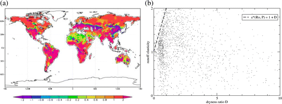
Rainfall induced runoff elasticity ε (Ro,P) simulated by ECHAM5 (20C and A1B): a Geographical and b dryness D dependent distributions (scatter plot); runoff elasticitiy ε* based on Schreiber’s formula (dashed)
-
(ii)
Note that net radiation dependent runoff elasticity can also be deduced, as ε*(Ro, N) = −D* satisfies the balance ε*(Ro, P) + ε*(Ro, N) = 1, if N and P are uncorrelated.

Attribution
Further insight into the runoff-rainfall processes which are underlying climate and basin change is gained by employing the Budyko framework (following Milne et al. 2002, Tomer and Schilling 2009, see also Renner et al. 2012). Utilizing relative excess rainfall and energy changes, dU and dW, provides estimates of change attribution. This is measured by the attribution-ratio (dU/dW) which, for the idealized rainfall-runoff chain (eqs. 5 and 6, see also Figs. 1a and 6b), yields (dU/dW)* ~ −1 in the dryness range, 0 < D* < 2 to 3, from Tundra via Forests and Steppe to Semi-deserts. Under the ideal conditions of watersheds in equilibrium, this has the following consequences: If an observed trajectory of change is aligned along the slope parallel to the off-diagonal in (U,W)-space, it can be attributed to (i) climate or external change; if it is aligned parallel to the main-diagonal, the change can be attributed to (ii) basin or internal change. That is, climate change represents the external forcing due to changing water and energy input, that is precipitation P and net radiation N (linked by dryness ratio D = N/P); internal (or land surface) changes are due to flux partitioning between evaporation and runoff and/or evaporation and sensible heat flux. These shifts in opposite directions in (W,U)-space are commonly deduced by the following ‘Gedanken’ experiment:
-
(i)
Climate change (dD) at fixed E (or Ro) corresponds to increasing (decreasing) net radiation and decreasing (increasing) precipitation, which is aligned along the off-diagonal in the (U,W)-diagram (Fig. 1a). That is, dU > 0 and dW < 0 (dU < 0 and dW >0). The idealized rainfall-runoff chain as reference climate shows that decreasing (increasing) dryness D* is associated with an increasing (decreasing) relative excess water W* (Eq. 3).
-
(ii)
Basin change is characterized by changes in the evapotranspiration from vegetation and/or soil. It introduces shifts in excess water W and energy U towards higher W and U, or lower W and U, respectively. That is, a change of the evaporation ratio, F = E/P, shifts excess rainfall, W = 1 – F, and excess energy, U = 1 – F/D, in the same directions along the main diagonal, which yields an attribution-ratio dU/dW ~ 1.
Figure 6 presents an application of the attribution analysis to changes in the IPCC4 scenario 20C GCM simulations from period-1 (1958–2001) to CO-2 conditions prescribed by A1B–scenario in the stabilization period-2 (2101–2144). First, climate states are presented by occupation frequencies of geographical grid points in (U,W)-state space (Fig. 6a,b), whose maxima are very broadly aligned along the ideal rainfall runoff chain. Changes are reflected by differences in density changing from period-1 (left) to period-2 (right): It appears that dry regions D > 1 tend to be enlarged with more ‘pixels’ being accumulated or ‘dry becomes drier’.

Global change (ECHAM5 A1B-scenario) in the (U,W)-state space in terms of number density of grid points for (a) period-1 (1958–2001) and (b) period-2 (2101–2144); attribution-ratio (tan−1 (dU/dW)) of relative excess energy dU and rainfall dW in the geographical space c and as dryness D dependent distribution of dU/dW (scatter plot) with runoff-rainfall attribution based on Schreiber’s formula (Eq.6 dashed)
Next, projecting the directions of these changes onto the geographical space shows locations of the attribution-ratio tan−1 (dU/dW) (Fig. 6c,d) linked to climate and basin induced causes. Ecohydrologic shifts can be associated with four basic combinations of change of relative excess energy U and water W supplies (Fig. 1): (i) Increasing (0° ~ 90°) or decreasing (−90° ~ −180°) represent a change in flux partitioning (say dE), affect the watershed due to a change in vegetation or soil and thus deviate from the slope of the main (positive) diagonal. (ii) Increasing W and decreasing U (−90° ~ 0°) or vice versa (90° ~ 180°) represents climate induced change along the negative diagonal. First, the attribution-ratio dU/dW combined with dryness D is presented as scatter plot (Fig. 6d) for the GCM-simulation and as functional relationship (Eq. 6) for the idealized rainfall-runoff chain representing a mean dU/dW for a mean D. Note the systematic bias of the idealized rainfall-runoff chain, which is also evident in the density distribution (Fig. 6a-b). Finally (Fig. 6c) shows the same results in the geographic space, for which the following points are noted: Global change induced by climate should be aligned along the slope (dU/dW ~ −1), accepting the scatter about dU/dW ~ 0, appears to dominate the GCM simulated change. The smaller areas attributed to basin induced change (dU/dW × 1, 0° ~ 90°, 90° ~ −180°) may be related to the energy and/or water storage still existing despite the long-term averaged simulations.
In summarizing we note that the idealized rainfall-runoff chain (Eq. 6, dashed line in Fig. 6d) separates the attribution of change from climate to basin induced processes as it is characterized by external forcing (of water and energy supply) and internal partitioning (of the sensible and latent heat fluxes and runoff). But systematic bias occurs when comparing the density distributions of both climate mean states (Eq. 5, see Fig. 6a-b) and analyzing the attribution of their changes (Eq. 6, see Fig. 6d) averages are associated with the idealized rainfall-runoff chain. This bias may be related to the energy and/or water storage change, which still exists when analyzing long-term or climate means of GCM-simulations.
5 Conclusion and Outlook
We have characterized the ecohydrology at the Earth’s surface by physical climate state parameters, based on Budyko’s (1974) framework using a set of non-dimensional water and energy flux ratios and an ecohydrological model of an ideal rainfall-runoff, which comprises an equation of state (based on a stochastic biased coinflip model) constrained by surface water and energy balance equations in equilibrium. This ideal rainfall-runoff chain simulates, on catchment scale, land surface hydro-climates in equilibrium (Schreiber 1904; Fraedrich 2010). It is validated within a coupled global climate model environment (supplementing a regional model analysis, Sun et al. 2013), because state of the art models provide physically consistent datasets. Validation analyses shows that, on catchment scale, the stochastic model indeed performs as a rainfall-runoff chain and can serve as a suitable low order model of the Earth’s near surface hydro-climate. Its main natural features are long term averages, variability and change, which provide measures on catchment and climate scale including vegetation, rivers (and lakes). Future tests to link global and regional change in climate and land use with climate and vegetation, in particular in the extreme climates of the Tibetan Plateau and South American Altiplano, are ongoing areas of research in particular, employing GCM alternatives for future climate estimates (Zhu et al. 2013) and remote sensing information (Cai et al. 2014).
In summarizing: Surface water resources modeling comprises a spectrum of models ranging from highly complex numerical to low order theoretical stochastic-dynamical systems. In this sense a low order model is introduced comprising the water and energy balance equations and an ideal rainfall-runoff chain, which is derived as an equation of state explaining an empirically discovered relationship (not unlike the derivation of the empirically discovered ideal Gas Law). Here we verify this model in a complex global climate model environment and results suggest it to be a useful tool for ecohydrological analysis of regional catchments and, possibly, prediction of ungauged basin.
References
Arora V (2002) The use of the aridity index to assess climate change effect on annual runoff. J Hydrol 265:164–177
Budyko MI (1974) Climate and Life, Academic Press, 508pp
Bordi I, Fraedrich K, Sutera A (2009) Observed drought and wetness trends in Europe: an update. Hydrol Earth Syst Sci 13:1519–1530
Cai D, Fraedrich K, Sielmann F, Guan Y, Guo S, Zhang L, Zhu X (2014) Climate and vegetation: An ERA-Interim and GIMMS NDVI analysis. J. Climate 27, doi:10.1175/JCLI-D-13-00674.1
Dooge JCI (1992) Sensitivity of runoff to climate change: a hortonian approach. Bull Am Meteorol Soc 73:2013–2024
Fraedrich K, Gerstengarbe FW, Werner PC (2001) Climate shifts in the last century. Clim Change 50:405–417
Fraedrich K (2010) A stochastic parsimonious water reservoir: Schreiber’s 1904 equation. J Hydromet 11:575–578
Fraedrich K, Sielmann F (2011) An equation of state for land surface climates. Int J Bifurcation Chaos 21:3577–3587
Hagemann SK, Arpe K, Roeckner E (2006) Evaluation of the hydrological cycle in the ECHAM5 model. J Clim 19:3810–3827
Hanasaki N, Kanae S, Oke T, Masuda K, Motoya K, Shirakawa N, Shen Y, Tanaka K (2008) An integrated model for the assessment of global water resources - Part 1: model description and input meteorological forcing. Hydrol Earth Syst Sci 12:1007–1025
Koeppen W (1936) Das geographische system der klimate – handbuch der klimatologie, Vol. 1, part C. Gebr. Borntraeger Verl, Berlin, p 388
Koster RD, Suarez MJ (1999) A simple framework examining the interannual variability of land surface moisture fluxes. J Clim 12:1911–1917
Milne BV, Gupta V, Restrepo C (2002) A scale invariant coupling of plants, water, energy, and terrain. Ecoscience 9:191–199
Renner M, Seppelt R, Bernhofer C (2012) Evaluation of water-energy balance frameworks to predict the sensitivity of streamflow to climate change. Hydrol Earth Syst Sci 16:1419–1433
Roeckner E, Lautenschlager M, Schneider H (2006) IPCC-AR4MPI-ECHAM5-T63L31MPI-OMGR1.5 L40 SRESA1B run no. 1: atmosphere monthly mean values MPImet/MaD Germany. World Data Cent Clim. doi:10.1594/WDCC/EH5- T63L31-OM-GR1.5L40-A1B-1-MM
Schreiber P (1904) Über die Beziehungen zwischen dem Niederschlag und der Wasserführung der Flüsse in Mitteleuropa. Meteorol Z 21:441–452
Sharif HO, Crow W, Miller NL, Wood EF (2007) Multidecadal high-resolution modeling of the Arkansas-Red River basin. J Hydromet 8:1111–1127
Sun R, Zhang X, Sun Y, Zheng Du, Fraedrich K (2013) SWAT-based streamflow estimation and its responses to climate change in Kadongjia River Watershed, South Tibet, China J Hydromet 1571–1585
Tao H, Borth H, Fraedrich K, Su B, Zhu X (2014) Drought and wetness variability in the Tarim River Basin and connection to large-scale summer atmospheric circulation. Intern J Climatology 34, doi:10.1002/joc.3867
Tomer MD, Schilling KE (2009) A simple approach to distinguish land-use and climate-change effects on watershed hydrology. J Hydrol 376:24–33
Wang Q, Takahashi H (1998) A land surface water deficit model for an arid and semiarid region: impact of desertification on the water deficit status in the Loess Plateau. China J Clim 12:244–257
Zhang L, Hickel K, Dawes WR, Chiew FHS, Western AW, Briggs PR (2004) A rational function approach for estimating mean annual evapotranspiration. Water Resources Research, 40, W02502, doi:10.1029/2003WR002710
Zhu X, Bothe O, Fraedrich K (2010) Summer atmospheric bridging between Europe and East Asia: influences on drought and wetness on the Tibetan Plateau. Quat Int 236:151–157
Zhu X, Wang W, Fraedrich K (2013) Future climate in the Tibetan Plateau from a statistical regional climate model. J Clim 23:10125–10138
Author information
Authors and Affiliations
Corresponding author
Rights and permissions
About this article

Cite this article
Fraedrich, K., Sielmann, F., Cai, D. et al. Validation of an Ideal Rainfall-Runoff Chain in a GCM Environment. Water Resour Manage 29, 313–324 (2015). https://doi.org/10.1007/s11269-014-0703-2
Received:
Accepted:
Published:
Issue Date:
DOI: https://doi.org/10.1007/s11269-014-0703-2