
Abstract
It is a remarkable fact that images are related to objects constituting them. In this paper, we propose to represent images by using objects appearing in them. We introduce the novel concept of object bank (OB), a high-level image representation encoding object appearance and spatial location information in images. OB represents an image based on its response to a large number of pre-trained object detectors, or ‘object filters’, blind to the testing dataset and visual recognition task. Our OB representation demonstrates promising potential in high level image recognition tasks. It significantly outperforms traditional low level image representations in image classification on various benchmark image datasets by using simple, off-the-shelf classification algorithms such as linear SVM and logistic regression. In this paper, we analyze OB in detail, explaining our design choice of OB for achieving its best potential on different types of datasets. We demonstrate that object bank is a high level representation, from which we can easily discover semantic information of unknown images. We provide guidelines for effectively applying OB to high level image recognition tasks where it could be easily compressed for efficient computation in practice and is very robust to various classifiers.
1 Introduction
High-level image recognition is one of the the most challenging domains in the field of computer vision. Any high-level image recognition task using computer vision algorithms starts with image representation, the process of turning pixels into a vector of numbers for further computation and inference. Of all the modules for a robust high-level image understanding system, the design of robust image representation is of fundamental importance and has been attracting many vision researchers. Compared to other data modalities, visual data is particularly challenging because of the extreme richness and diversity of the contents being captured in real world, and the large variability in photometric and geometric changes the real world could map onto the 2D pixel world. Pixels, unlike other information carriers such as words, carry very little meaning themselves, and are extremely volatile to noise. In the past decade, a great amount of research has been conducted on developing robust image representation. Among the image representations widely adopted so far, most of them are low level image representations focusing on describing images by using some variant of image gradients, textures and/or colors [e.g. SIFT (Lowe 1999), filterbanks (Freeman and Adelson 1991; Perona and Malik 1990), GIST (Oliva and Torralba 2001), etc.]. However, there exists a large discrepancy between these low level image representations and the ultimate high level image recognition goals, which is the so called ‘Semantic gap’. One way to bridge the semantic gap is by deploying increasingly sophisticated models, such as the probabilistic grammar model (Zhu et al. 2007), compositional random fields (Jin and Geman 2006), and probabilistic models (Fei-Fei and Perona 2005; Sudderth et al. 2005). While these approaches are based on rigorous statistical formulation, good learning and inference are still extremely difficult. Most of the papers have shown promising results only on small scale datasets. It still remains a very challenging task for the models to bridge the low level representations and the high level visual recognition tasks.
One notable development in image representation is the recent work that explores to build image representations using intermediate ‘attributes’ (Ferrari and Zisserman 2007; Lampert et al. 2009; Farhadi et al. 2010; Torresani et al. 2010). Its success in recognition is largely accredited to the introduction of ‘attribute’, a high-level semantically meaningful representation effectively summarizing the low-level image properties. In attribute-based methods for object recognition, an object is represented by using visual attributes. For example, a polar bear can be described as white, fluffy object with paws. Such visual attributes summarize the low-level features into object parts and other properties, and then are used as the building blocks for recognizing objects in test images. In the work of Ferrari and Zisserman (2007), the authors developed a topic model to learn the mapping of low-level image properties to predefined color and shape attributes. Similarly, Lampert et al. (2009) and (2010) propose to detect and describe objects in unknown images based on their correlation with a set of human-specified high-level descriptions of the target objects. Attribute-based methods have demonstrated great potential in image classification as well. For example, in Torresani et al. (2010), the authors build a high-level image representation from a collection of classifier results and achieved promising results.
On the other hand, using global/local structure information has proved to be useful to increase the descriptive power of a representation. For example, by applying spatial pyramid structure to bag of words (BoW) representation, Lazebnik et al. (2006) proposed the Spatial Pyramid Model that gives superior performance compared to the original BoW features.
Image representations based on either attribute and spatial location have demonstrated potential in visual recognition tasks, which reminds us how human interprets an image. What will pop up in your mind when imagining a sailing scene? We often think of sailboat, ocean and blue sky, each at some specific location. Objects are essential components to interpret an image. As human, we start to learn numerous objects from our childhood and memorize the appearance of learned objects. Their appearance are then used to effectively describe our visual world.
Therefore, we hypothesize that object appearance and their spatial locations could be very useful for representing and recognizing images. In this paper, we introduce object bank (OB), a novel high level image feature to represent complex real-world image by collecting the responses of many object detectors at different spatial locations in the image. Drawing an analogy to low-level image representation, instead of using image filters to represent local texture, we introduce object filters to characterize local image properties related to the presence/absence of objects. By using a large number of such object filters, our object filter bank representation of the image can provide rich information of the image that captures much of the high-level meaning. OB is a compact structure to encode our knowledge of objects for challenging high level visual tasks in real world problems such as image classification. OB is a high level image representation that provides probability of objects appearing in images and their spatial locations as the signature of images.
As a proof of concept, we apply OB to high level image classification tasks by using simple, off-the-shelf classifiers. It delivers promising image recognition results on various benchmark datasets and outperforms significantly over all existing traditional low level features. In this paper, we provide in-depth analysis of each component in OB and simple guidelines on effectively applying OB representation to image classification task. We show that, by encoding semantic and spatial information of objects within an image, OB can not only achieve state-of-the-art performance in high level visual recognition tasks but also discover meaningful aspects of objects in an image. To explore its potential in practice, we analyze the robustness and efficiency of object bank. We show that OB is robust to different off-the-shelf classifiers. For large scale computation, OB can be easily compressed to compact representation while preserving its robustness.
2 Related Work
A considerable body of research has been focusing on using traditional low level image features for image classification, such as filter banks (Leung and Malik June 2001; Perona and Malik 1990; Freeman and Adelson 1991), GIST (Oliva and Torralba 2001), and BoW of local features (Bosch et al. 2006; Fei-Fei and Perona 2005). Instead of using gradients or colors in an image to represent it, OB characterizes local image properties by using object filters related to the presence/absence of objects, adding more high level information into the representation to bridge the semantic gap.
Object detection and recognition also entail a large body of literature (Fei-Fei et al. 2007; Bourdev and Malik 2009). Promising object detectors have been introduced by Felzenszwalb et al. (2007), as well as the geometric context classifiers (‘stuff’ detectors) of Hoiem et al. (2006). These object recognition approaches accelerate the advancement of new state-of-the-art object detection and classification algorithms such as Desai et al. (2009) and Song et al. (2011).
Visual attributes based research for image recognition (Farhadi et al. 2010; Ferrari and Zisserman 2007; Lampert et al. 2009; Torresani et al. 2010) has achieved substantial progress recently. These approaches focus on single object classification based on visual attributes. The pre-defined concepts used in Lampert et al. (2009), Farhadi et al. (2010) and Torresani et al. (2010) are not necessarily directly related to visual pattern in the images, e.g. ‘eats fish’ in Lampert et al. (2009), ‘carnival’ in Farhadi et al. (2010) and ‘able-minded’ in Torresani et al. (2010). Different than these approaches, OB representation encodes semantic and spatial information of objects universally applicable for high level visual recognition tasks. Among these approaches, the closest to object bank is proposed by Torresani et al. (2010), where a compact descriptor is learned from a set of pre-trained concept classifiers. While the classmes representation proposed by Torresani et al. (2010) underscores the compactness of a feature representation for large scale visual tasks, we advocate a rich image representation encoding semantic and spatial information for inferring semantic and structural relationship from.
The idea of using object detectors as the basic representation of images is related to work in multimedia by applying a large number of ‘semantic concepts’ to video and image annotation (Hauptmann et al. 2007). However, in Hauptmann et al. (2007), each semantic concept is trained by using the entire images or frames of video. Understanding cluttered images composed of many objects will be challenging since there is no localization of object concepts in images in this approach.
In Vogel and Schiele (2004), a handful number of concepts are learned for describing an image. For each location, only the most probable concept is used to form the representation based on binary classification result. Significant amount of information is lost during their feature extraction process. Our approach, on the other hand, encodes the probabilities of all objects candidates appearing in all locations in the image resulting in much richer image representation.
Recently, feature learning approaches have made great progress in image classification by building advanced machine learning models to learn from low level feature representation (Dixit et al. 2011; Gao et al. 2010, 2011). Most of these approaches learn useful feature representations from low level image features such as visual code word of SIFT (Lowe 1999). By encoding rich content of semantic and spatial information, OB can serve as a potential complimentary feature pool for these algorithms to learn more sophistic image representation from.
3 The OB Representation of Images
In this section, we introduce the concept of high-level OB representation (Li et al. 2010a, b). The ultimate goal of OB representation is to capture as much objects information contained in the images including their semantic meaning, spatial locations, sizes and view points etc. as possible. We achieve this by constructing OB, a collection of object filters trained on multiple objects with different view points.
3.1 Construction of the OB
So what are the “objects” to use for constructing the OB? And how many? An obvious answer to this question is to use all objects. As the detectors become more robust, especially with the emergence of large-scale datasets such as LabelMe (Russell et al. 2005) and ImageNet (Deng et al. 2009), this goal becomes more reachable.
But time is not fully ripe yet to consider using all objects in, say, the ImageNet dataset. Not enough research has yet gone into building robust object detector for tens of thousands of generic objects. As we increase the number of objects, the issue of semantic hierarchy becomes more prominent. Not much is understood about what it means to detect a mammal and a dog simultaneously. And even more importantly, not all objects are of equal importance and prominence in natural images. As Fig. 1 shows, the distribution of objects follows Zipf’s Law, which implies that a small proportion of object classes account for the majority of object instances. Hauptmann and colleagues have postulated that using 3,000–4,000 concepts should suffice to annotate most of the video data (Hauptmann et al. 2007).

(Best viewed in colors and magnification) The frequency (or popularity) of objects in the world follows Zipf‘s law trend: a small proportion of objects occurs much more frequently than the majority. While there are many ways of measuring this, e.g., by ranking object names in popular corpora such as the American National Corpora (2001) and British National Corpus Edition and Sampler, we have taken a web-based approach by counting the number of downloadable images corresponding to object classes in WordNet on popular search engines such as Google, Ask.com and Bing. We show here the distribution of the top 2,000 objects
In this paper, we choose a few hundred most useful (or popular) objects in images.Footnote 1 An important practical consideration for our study is to ensure the availability of enough training images for each object detectors. We therefore focus our attention on obtaining the objects from popular image datasets such as ESP (Ahn 2006), LabelMe (Russell et al. 2005), ImageNet (Deng et al. 2009) and the Flickr! online photo sharing community. After ranking the objects according to their frequencies in each of these datasets, we take the intersection set of the most frequent 1,000 objects, resulting in 177 objects, where the identities and semantic relations of some of them are illustrated in Fig. 2. To train each of the 177 object detectors, we use 100\(\sim \)200 images and their object bounding box information from the ImageNet (Deng et al. 2009) datasets.

(Best viewed in colors and magnification) Rough grouping of the chosen object filters based loosely on the WordNet hierarchy (Miller 1995). The size of each unshaded node corresponds to the number of images returned by the search. The list of objects used in object bank is available at http://vision.stanford.edu/projects/objectbank/objectlist.txt
To our knowledge, no previous work has applied more than a handful of object detectors in scene recognition tasks (Desai et al. 2009). But our initial object filter bank of 177 object detectors is still of modest size. We show in Sect. 4 that even with this relatively small number of objects we can achieve promising recognition results (e.g., Fig. 5).
3.2 The OB Representation
Figure 3 illustrates our OB representation construction process. Given an image, an object filter response can be viewed as the response of a ‘generalized object convolution.’ We obtain object responses by running a bunch of object filters across an image at various locations and scales by using the sliding window approach. Each filter is an object detector trained from images with similar view point. If not specified, we apply the deformable part based model from Felzenszwalb et al. (2007) as our object detector where six parts are used. For each scale and each detector, we obtain an initial response map, whose value at each location indicates the possibility of the occurrence of that object. To capture the spatial location property of objects, we build a spatial pyramid for the response map. At each layer of the spatial pyramid structure, we extract the signal from all grids. Finally, we build the OB representation by concatenating all the extracted responses.

(Best viewed in colors and magnification) Illustration of the object filter representations. Given an input image, we first run a large number of object detectors at multiple scales to obtain the object responses, the probability of objects appearing at each pixel. For each object at each scale, we apply a three-level spatial pyramid representation of the resulting object filter map, resulting in \(\mathtt {No.Objects} \times \mathtt {No.Scales} \times (1^2+2^2+4^2)\) grids. An OB representation of an image is a concatenation of statistics of object responses in each of these grids. We consider three ways of encoding the information. The first is the max response representation (OB-Max), where we compute the maximum response value of each object, resulting in a feature vector of \(\mathtt {No.Objects}\) length for each grid. The second is the average response representation (OB-Avg), where we extract the average response value in each grid. The resulting feature vector has the same length as the maximum response. The third is the histogram representation (OB-Hist). Here for each of the object detectors, we keep track of the percent of pixels on a discretized number of response values, resulting in a vector of \(\mathtt {No.BinnedResponseValues} \times \mathtt {No.Objects}\) length for each grid
Max Response Representation (OB-Max, Fig. 3). As shown in Fig. 3, OB-Max encodes the strongest object filter response at each grid and each level of the spatial pyramid and detector scale. In our case, we have 177 objects, 12 scales (six scales from each of the two components) and 21 spatial pyramid grid (L = 2), which is in 44,604 dimension in total. In the example image shown in Fig. 3, given the OB-Max representation, the possibility of sailboat and water appearing in that specific grid is higher than other objects. If not specified, OB-Max is the default OB pooling method in our following experiments.
Average Response Representation (OB-Avg in Fig. 3). OB-Avg encodes the average object filter response at each grid and each level of the spatial pyramid and detector scale. From the responses to different object filters, we form the OB feature by representing the (scene/event) image as a vector of average values from each spatial pyramid grid.
Histogram Response Representation (OB-Hist, Fig. 3). OB-Hist captures more detailed information of the object filters than OB-Max. Instead of using maximum response value of each object detector in each grid of the spatial pyramid representation of each of the response map, we construct a histogram of the responses in each grid. The histogram has a vector length of the number of objects, and the value of each bin is indicated by the number of pixels with the response value within that bin. Four histogram bins in each grid are used in the experiment. As the example in Fig. 3 illustrates, within that specific grid, most response values of sailboat detector are high whereas most response values of bear detector are low.
Before we apply OB representation for visual recognition tasks, we first ask whether this representation encodes discriminative information of images. In Fig. 4, we compare the OB image representation to two popular low-level image representations: GIST (Oliva and Torralba 2001) and the spatial pyramid (SPM) representation of SIFT (Lazebnik et al. 2006). The low-level feature responses of the two images belonging to different semantic classes are shown to be very similar to each other, whereas the OB features can easily distinguish such scenes due to the semantic information provided by the object filter responses. In Sect. 4, the discriminability of our OB representation is further supported by a series of comparison to the state-of-the-art algorithms based upon low-level image representation on high level visual recognition tasks. In this series of comparison, if not specified, we use the OB-Max representation with plain logistic regression classifier.

(Best viewed in colors and magnification) Comparison of object bank representation with two low-level feature representations, GIST and SIFT–SPM of two types of images, mountain versus city street. For each input image, we first show the selected filter responses in the GIST representation (Oliva and Torralba 2001). Then we show a histogram of the SPM representation of SIFT patches (Lazebnik et al. 2006) at level 2 of the SPM representation where the codeword map is also shown as a histogram. Finally, we show a selected number of object filter responses
4 High Level Visual Recognition by Using Different Visual Representations
As we try to tackle the high level visual recognition tasks, the semantic gap between low-level features and high-level meanings becomes big. One solution to this is to use complex models to pool in information (Sudderth et al. 2005; Li and Fei-Fei 2007; Tu et al. 2005; Li et al. 2009). But the drawbacks are clear. Researchers have to put large amount of effort to design such complex models. Due to the complexity, they might not scale well with large scale data or different datasets. In addition, some models (Sudderth et al. 2005; Li and Fei-Fei 2007) require extra amount of supervision, which causes such models to be impractical. Can we leverage on relatively simple statistical models and classifiers, but try to develop descriptive image representation to narrow the semantic gap better? We hypothesize that by introducing features that are ‘higher level’, such as OB, we could do this.
While it is good to see a clear advantage of discriminative power of OB over the low level image representations visually, we want to further examine its potential in high level visual recognition tasks on multiple benchmark datasets. In our experiments, we use simple off-the-shelf classifiers to dissect the contribution of the representations in classification. We compare to related image representations as well as the state-of-the-art approaches built upon them directly with more complex models. Scene classification performance is evaluated by average multi-way classification accuracy over all scene classes.
4.1 OB on Scene Classification
Before we describe the experiment details, we first introduce the four benchmark scene datasets used in our scene classification experiment, ranging from generic natural scene images [15-Scene (Lazebnik et al. 2006), LabelMe 9-class scene dataset (Li et al. 2010a)], to cluttered indoor images [(MIT Indoor Scene (Quattoni and Torralba 2009)], and to complex event and activity images [UIUC-Sports (Li and Fei-Fei 2007)]. For each dataset, we follow the settings in the paper introduced it and train a multi-class linear SVM and plain logistic regression classifiers.
Figure 5 summarizes the results on scene classification based on OB and a set of well known low-level feature representations: GIST (Oliva and Torralba 2001), BoW (Csurka et al. 2004) and Spatial Pyramid Matching (SPM) (Lazebnik et al. 2006) built upon the SIFT feature (Lowe 1999) on four challenging scene datasets. We also compare the performance of a simple linear SVM model and plain logistic regression built upon OB representation to the related algorithms on each benchmark datasets, demonstrating that a semantically meaningful representation can help to reduce the burden of sophisticated models for bridging the ‘semantic gap’ between high level visual recognition tasks and low level image representation.Footnote 2 We achieve substantially superior performances on three out of four datasets comparing to the traditional feature representations and algorithms built upon them directly, and are on par on the 15-Scene dataset. By combining multiple features, Pandey and Lazebnik (2011) recently proposes with classification accuracy of \(43.1\,\%\) on the MIT-Indoor dataset which is slightly lower than that obtained by the best performed OB representation OB-Hist (\(47.1\,\%\) in Fig. 13). It is worth mentioning that recent feature learning approaches have achieved superior performance in image classification by building advanced machine learning models to learn from low level feature representation (Dixit et al. 2011; Gao et al. 2010, 2011; Bo et al. 2011). For example, Gao et al. (2011), Dixit et al. (2011), Gao et al. (2010) and Bo et al. (2011) achieved classification accuracy of \(79.37\), \(84.4\), \(84.92\) and \(85.7\,\%\) respectively on the UIUC-Sports dataset.Footnote 3 While these powerful machine learning approaches are built upon low level feature representations, OB can serve as a potential complimentary feature source with rich content of semantic and spatial information for them to learn more sophistic image representation from. Ideally, better result could be achieved by combining multiple types of features from previous successful examples such as Varma and Zisserman (2003). However, it is beyond the scope of this paper to discuss feature learning from OB and other low level features.
The advantage of OB is especially obvious when the images are highly cluttered by objects. Its substantial performance gain on the UIUC-Sports and the MIT-Indoor scene datasets illustrates the importance of using a semantically meaningful representation for complex scenes cluttered with objects. For example, the difference between a living room and a bedroom is less obvious in the overall texture (easily captured by BoW or GIST), but more significant in the different objects and their arrangements. This result underscores the effectiveness of OB, highlighting the fact that in high-level visual tasks such as complex scene recognition, a higher level image representation can be very useful.
4.2 OB on Object Recognition
A fundamental task in high level visual recognition is object recognition, in particular, generic object categorization. Generic object categorization is a challenging task owing to the various appearance and locations of objects in the images. OB is constructed from the responses of many objects, which encodes the semantic and spatial information of objects within images. It can be naturally applied to object recognition task. We test its object recognition ability on the Caltech 256 dataset (Griffin et al. 2007). We compare to classemes (Torresani et al. 2010), an attribute based representation obtained as the output of a large number of weakly trained concept classifiers on the image without considering the spatial location and semantic meaning of objects. As described in Torresani et al. (2010), classeme extractors are 2,659 object classifiers learned from images retrieved by Bing Image Search. Similar to our approach, classemes (Torresani et al. 2010) consists of two distinct stages: a once-only feature learning stage and a classifier learning stage. We follow the training and test setting of the key comparison in the classemes paper (Torresani et al. 2010) by using exact the same set of 30 training images and 25 test images from each of the 256 classes as Torresani et al. (2010) does. We compare the reported result in Torresani et al. (2010) to ours (Table 1).
By encoding the spatial locations of the objects within an image, OB significantly outperforms (Torresani et al. 2010) on the 256-way classification task, where performance is measured as the average of the diagonal values of a 256\(\times \)256 confusion matrix. Note that there are state-of-art algorithms perform better than both Object Bank and classemes by using advanced machine learning techniques (Gehler and Nowozin 2009; Perronnin et al. 2010; Wang et al. 2010). However, comparison to these algorithms is beyond the scope of this paper since our focus here is to evaluate the representation power of image features without using complex machine learning techniques. The improvement of OB over classemes demonstrates the importance of rich spatial information of objects and semantic meaning of objects encoded in OB. On the other hand, in the efficiency comparison, the computation cost of OB is between that of classemes’ and Gehler and Nowozin (2009) where classemes is significantly more efficient than OB and object bank is much more efficient than Gehler and Nowozin (2009) in both training and test.Footnote 4 This observation underscores the fact that OB advocates a rich image representation encoding both spatial and semantic properties whereas classemes focuses more on the compact, efficient properties of an image representation. Therefore, classemes has the advantage for large scale computation and OB serves better as a representation resource for algorithms to learn relationships or representative features. In Sect. 5.7, we provide a simple example of learning object–object and object–scene relationship from OB.
In Sect. 5, we analyze the effectiveness of both the semantic and spatial properties in detail and demonstrate the advantage of using rich spatial information and semantic meaning of objects. We further illustrate interesting patterns of object relationships discovered from our OB representation, which can serve as potential contextual information for sophistic models for high level visual tasks such as object detection, segmentation and scene classification.
5 Analysis: Role of Each Ingredient
In this section, we thoroughly analyze the role of each important component of our OB representation in a systematical fashion. We demonstrate the designing rationale of OB representation, the influence of detector quality and different components of OB, and eventually provide a good understanding of OB and how to construct a good OB representation.
The ideal object filters is capable of capturing object appearance accurately without losing significantly useful information during the process of construction. Here, we investigate the effectiveness of different designing choices. Specifically, we evaluate the effectiveness of these designing choices by measuring the classification performance of their resulting representation on different datasets.
-
1.
A robust object detector is able to produce accurate responses of the object indicating the probability of its appearance at each pixel in an image. We first examine the quality of different object detection algorithms (Dalal and Triggs 2005; Felzenszwalb et al. 2007) as the appearance object filters.
-
2.
Object view points vary over a wide range in different images. Multiple view points are essential for training our object filters to capture the multiple views of objects. We evaluate the effectiveness of the filters trained from different view points.
-
3.
Object sizes could differ significantly in different images. We run object filters at different scales to incorporate responses of multiple object sizes. We examine the effectiveness of different scales and the accumulated scales with an emphasis on the importance of using multiple scales.
-
4.
To capture the various locations of objects in images, we apply a spatial pyramid structure over the responses generated by object filters. We analyze the necessity of constructing the spatial pyramid structure.
-
5.
Our OB representation is a collection of statistics based upon responses to the object detectors. In addition, we examine the influence of different pooling methods on extracting the statistics from the response map.
-
6.
Objects are the most critical designing component in our OB representation. Finally, we analyze different schemes for selecting objects for the OB construction.
In the following experiments, we measure the importance of each component based on its contribution to recognition of scene images in different benchmark datasets. If not specified, we employ simple plain logistic regression as the classifier. Classification performance is obtained from fivefold random sampling of the training and testing examples. When examining one aspect of the OB representation, other aspect settings are fixed.
5.1 Comparison of Different Types of Detectors
The first question is what type of object detectors/filters we should use in OB. We are interested in examining the difference between a more sophisticate object detector LSVM (Felzenszwalb et al. 2007) and a simple object detector (Dalal and Triggs 2005). We first compare how well the detectors capture the object appearance based upon detection performance of LSVM and Dalal and Triggs on object categories from the ImageNet dataset. In the left panel of Fig. 6, we show that LSVM outperforms Dalal and Triggs in detecting objects in the ImageNet dataset.

Left Detection performance comparison of different detection methods on ImageNet objects. Right Classification performance of different detection methods on the UIUC sports dataset and the MIT Indoor dataset
As demonstrated in left panel of Fig. 6, the performance of OB based on stronger object detectors (LSVM) is better than that of OB representation based on Dalal anf Triggs. This reflects that a strong object detector captures the object identity and location in an image more accurately, hence provides better description of an image. This rule applies even though the objects in the OB do not entirely overlap with those appear in the scene images. In Fig. 6 (right), we envisage the OB will become better as more accurate object detection algorithms are developed. In the ideal case, if we use a perfect object detector, we can achieve much better performance in semantically separatable dataset. An interesting observation is that if we use the names of objects appear in each image from the UIUC sports dataset as the feature, we can achieve 100 % in classification accuracy by using a simple linear SVM classifier. On the other hand, there are objects sharing common properties such as the legs of a horse and a cow. Although objects in the OB could be different than those appear in the scene images, a better object detector can serve as a more accurate generic parts describer to transfer the knowledge learned from one object to another.
5.2 Role of View Points
The view points of objects in different images could vary dramatically. For example, in Fig. 7, rowing boats appear in different view points depending on the sceneries the photographers want to snap.

Diverse views of rowing boats in different images. Images are randomly selected from the UIUC sports dataset
In order to capture this property, we train the object detectors by using object images with different view points. To show our design rational on view points, we apply OB generated from objects with front view, side view and the combination of both to a scene classification task.
Demonstrated in the comparison (left panel of Fig. 8), front view contributes more in classification experiments on both datasets than side view of objects. Combining the two views further boosts classification performance on MIT Indoor dataset,Footnote 5 which shows that combining multiple view points is useful.
To verify our assumption and further investigate the effectiveness of combining multiple view points, we conduct a control experiment by training and testing on different views of one specific object. We select ‘rowing boat’ as an example since it has diverse view points.
As the panel on the right of Fig. 8 demonstrated, representation generated from only front view or side view performs reasonably well on test images with similar view points. OB representation, by incorporating both views, significantly outperforms these two baselines on all three types of testing images with different view points.
5.3 Role of Scales
Object size in different images could be very different, we therefore run object filter on different image scales to accurately capture this. In this experiment, we evaluate the importance of generating responses of objects at multiple scales in OB. We compare classification performance by using OB representation corresponding to each individual scale and multiple scales.
From Fig. 9, we observe that individual scales perform similarly to each other with the medium size scale consistently delivers the best result on both the UIUC sports and the MIT Indoor datasets. Our observation reflects that our object detector captures the medium size objects within these two datasets the best. This observation aligns well with the majority object sizes in ImageNet images. Each individual scale cannot capture all the variances but can already perform relatively well on this dataset. Same applies to MIT Indoor dataset. We further show an accumulative concatenation of scales. Figure 10 shows that incorporating multiple scales is helpful since it captures the variance of object sizes in the datasets. The classification accuracy keeps increasing when different scales are incorporated in the OB representation.

Classification performance on the UIUC sports event dataset (left) and the MIT Indoor dataset (right) by using object bank representation corresponding to each single scale. X axis is the index of the scale from fine to coarse. Y axis represents the average precision of a 8-way classification

Classification performance on the UIUC sports event dataset (left) and the MIT Indoor dataset (right) by using object bank representation corresponding to accumulated scale. X axis is the index of the scale from fine to coarse. Y axis represents the average precision of a 8-way classification
Objects could have significantly different sizes even they belong to the same object class. Here, we demonstrate that OB is able to capture the scale variance. In this control experiment, we assign the images in the ‘ball’ class into six scale groups based on the object size within the image. Same number of background images are randomly selected from the ImageNet object images. Representation generated from each individual scale and the combined ones are tested on a held out set of testing images with subgroups separated in a similar fashion. In addition, we simulate the real-world scenario by collecting a mixed test set of multiple object size images. In a similar manner, we generate the OB representation based upon responses to combination of all scales. We conduct binary classification by using the OB representation from each size group versus those of the background image group. Our experiment shows that the diagonal of Fig. 11 is much brighter than the off diagonal ones, which indicates that OB representation generated from each individual scale recognizes objects with similar size significantly better than the one generated from different size. In addition, the last row is much brighter than all the other grids, reflecting combination of all scales performs the best on different types of images. This again supports our design choice of incorporating multiple scales in OB representation.

Binary classification experiment for each individual scale and the combination of them. Each grid is filled in with ‘ball’ in different size. Each row represents a model trained on images with relatively similar scale (from small to large horizontally. Last row is the combination of all scales). Each column represents a test set with relatively similar scale. The more transparent the mask is, the better the classification accuracy is
5.4 Role of Spatial Location
Besides object semantic meaning, spatial locations of objects are critical for describing an image too. For example, ‘sky’ always appears in the upper part of an image whereas ‘water’ is always at the bottom. If the response of ‘sky’ has higher values in the upper part of an image, it adds more evidence that there is ‘sky’ in the image. To capture the spatial properties of objects in an image, we apply the spatial pyramid structure on the response map. In this experiment, we analyze the effectiveness of the spatial pyramid structure.
From the experiment, we observe similar pattern as observed in Lazebnik et al. (2006) except for the good performance by using level 0 on the UIUC sports dataset. In Table 2, we show that by using the maximum response from only level 0 as object bank representation (1/21 of the original dimension), we can achieve 81.1 % on the UIUC sports dataset. This reflects that in the UIUC sports dataset, semantic meaning alone is very discriminative. As long as we see a horse, no matter where it appears, it is able to differentiate polo scene from other scene types. On the other hand, adding spatial information does improve the classification performance with a small margin indicating the effectiveness of spatial location information of object.
Spatial location is critical in separating different indoor images. For example, computer room and office could both have computers, desks and chairs. But the number of instances and the spatial location arrangement of them could be quite different. OB representation encoding spatial location is able to capture such difference and hence generates better performance in classification. Our classification experiment on MIT Indoor dataset shows that by encoding spatial location, OB representation significantly outperforms the one only contains semantic information (level 0 result).
To further demonstrate the effectiveness of the spatial location component in the OB representation, we conduct a spatial location control experiment. In this experiment, we select an object that always appear at the top of the image, e.g. ‘cloud’ and an object that always appear at the bottom of the image, e.g. ‘grass’. We use level 2 in the spatial pyramid structure as an example, each time we preserve one of the spatial location as the representation and perform classification based on OB feature extracted from it alone. In Fig. 12, we show the heat map generated by using the smoothed classification score of the object at each spatial location.Footnote 6 Red color indicates high classification accuracy whereas blue represents low classification accuracy at that area. We observe that the OB representation generated from regions with high performance are also the locations where the object frequently appears. For example, cloud usually appears in the upper half of a scene in the beach class whereas grass appear at the bottom.
5.5 Comparison of Different Pooling Methods
As described earlier, OB representation is summarized from the responses of the image to different object filters. In order to obtain the geometric locations and semantic meaning of objects, we extract statistics of object appearance from different spatial locations by using pooling methods. The quality of pooling method influence the information that the OB representation carries. In a similar vain, we analyze the effectiveness of different pooling methods. Specifically, we focus on the three types of OB representations introduced in Sect. 3 obtained by using different pooling methods: average pooling (OB-Avg), max pooling (OB-Max) and histogram pooling (OB-Hist). We fix other designing choices in our OB and use the same classifier for different pooling methods.
One concern is that the richness of the representation could be attributed to the high dimension of features. To investigate this possibility, we compress the three representations to the same dimension by using PCA and perform classification on the compressed representation.
Figure 13 (left) shows that object bank representation generated from histogram pooling performs the best in classification. Figure 13 (right) illustrates that OB-Hist performs the best even when it is compressed to the same dimension as the other two methods. It indeed carries more information that is more descriptive of the images.

Left Classification performance of different pooling methods. Right Classification performance of PCA projected representations by using different pooling methods. Dimension is fixed to the minimum number of principal components to preserve 99 % of the unlabeled data variance of the three representations. Average and maximum response values within each spatial pyramid grid are extracted as the object bank feature in average pooling and max pooling respectively. We discretize values within each spatial pyramid to construct the histogram pooling representation
5.6 Role of Objects
We have introduced in Sect. 3 that object bank is built upon image responses to a group of pre-trained object detectors. Object candidates are very critical component in designing the OB representation. In this subsection, we analyze the effectiveness of different types of objects. Specifically, we are interested in OB generated from a generic pool of objects, a specific list of semantically related objects, a subgroup of objects with good detection performance, and a small group customized objects which are directly related to scene images.
5.6.1 Generic OB
We first examine the generic OB representation constructed from 177 most popular objects from ImageNet described in Sect. 3. We first investigate how well each individual object is able to capture the essential information within images, evaluated by the classification performance of object bank representation generated from each individual object. In Fig. 14, each dot represents the classification performance of a specific object. The first observation is that the classification precisions across single objects are not necessarily correlated with the detection performance (objects are sorted by their detection performance from high to low). This can be attributed to the fact that the objects with good detections might not have semantic relationship with the scene types we test on. In general, the performance over a single object falls in the 40–60 % range for the UIUC sports dataset, which indicates that the information captured by a single object is quite significant. However, it is still far from explaining away the information provided by combination of information from all objects, i.e., the full-dimensional OB representation.

Left Classification performance on the UIUC sports event dataset by using object bank representation corresponding to each single object. Right Classification performance on the MIT Indoor dataset by using object bank representation corresponding to each single object. X axis is the index of the object sorted by using the detection performance on object datasets from ImageNet. Y axis represents the average precision of a 8-way classification
To investigate the effectiveness of using multiple object candidates in OB, we vary the number of object candidates and test the resulting representation on scene classification. By plotting the average precision where an OB feature corresponding to a subsequent object is added one at a time in Fig. 15, we observe that the classification accuracy increases along with the increase of number of objects on both datasets. We believe that future growth of OB will lead to stronger representation power and more discriminative images models build on OB.

Classification performance on the UIUC sports event dataset and the MIT Indoor dataset by using object bank representation corresponding to accumulative object. X axis is the number of objects. Y axis represents the average precision of a 8-way classification
5.6.2 How Much Semantic Meaning and Appearance Helps: Customized OB
In the ideal case, if we know the identity of objects in each image and use them directly as the image representation, the classification performance on the UIUC sports event dataset is 100 %. Models that accurately predict the semantic meaning of objects can serve as critical prior knowledge for describing an image. An important characteristics of OB representation is that it encodes prior knowledge of objects. Here, we analyze the influence of prior knowledge especially the semantic meaning and appearance knowledge of objects encoded in OB representation generated by using a group of customized objects.
We begin with investigating the appearance models, i.e. our object filters, trained from both the ImageNet and the UIUC training images. We show below comparison of object filters trained on two candidate objects, ‘sail boat’ and ‘human’. We illustrate the models visualization comparison of these two objects.
As shown in Fig. 16, models trained on the UIUC training images capture a clearer shape of the objects.

Model comparison of ‘sail boat’ and ‘human’ models trained on the UIUC training images (left) and the ImageNet images (right)
The model quality is also reflected by their object detection performance on objects within the the UIUC scene test images.
In Fig. 17, we show that by clearly depicting the object appearance, models trained on the UIUC detects the objects in the object images in a held-out set accurately.

Detection performance comparison of models trained on the UIUC training images and ImageNet images
In addition, we compare the image classification performance by using only these models.
Figure 18 illustrates that the customized object bank models captures the object property better, which leads to better detection accuracy and better classification performance. Individual customized object models exhibit great potential in generating more descriptive image representation, we further verify the potential of customized object models of all semantically related objects in the the UIUC sports dataset.

Classification performance on the UIUC sports event dataset by using object bank representation generated from sailboat and human models trained on the UIUC training images and the ImangeNet images respectively. Y axis represents the average precision of a 8-way classification
We compare the overall classification performance by using all semantically related models, where we train the customized OB filters by using 25 object candidates Footnote 7 from the UIUC training images. We construct the customized OB representation based on these filters, called UIUC-25. UIUC-25 carries knowledge of object appearance from UIUC training images whereas the generic OB representation (ImageNet-177) encodes prior knowledge of object appearance from the ImageNet object training images. We compare UIUC-25 to ImageNet-177, Object Bank representation constructed from a subset of randomly selected 25 objects (ImageNet-25) as well as the ‘pseudo’ OB representation generated from a set of synthesized models neglecting the semantic meaning of objects.
In Fig. 19 (left), while the generic OB (ImageNet-177 and ImageNet-25) has very good generalizability, the customized OB consistently delivers much better result. It not only outperforms OB generated from equivalent number of object candidates in ImageNet, but also outperforms full dimensional OB. It is worth noticing that the dimension of full dimensional OB is over seven times that of the customized OB representation. Comparing to Li and Fei-Fei (2007), which requires labels of each pixel within an image in training, customized OB outperforms it significantly without additional information required. In fact, obtaining bounding box costs less labor than obtaining object contour required in Li and Fei-Fei (2007). We further decompose the spatial structure and semantic meaning encoded in OB by using a ‘pseudo’ OB without semantic meaning. The significant improvement of OB in classification performance over the ‘pseudo OB’ is largely attributed to the effectiveness of using object detectors trained from image. On the other hand, ‘pseudo’ OB performs reasonably well indicating that it does capture consistent structures in the images. To demonstrate the capabilities of different models in encoding the structural information in images, we show the models and their corresponding response maps in Fig. 20.

Left Classification performance on UIUC sports event dataset by using UIUC-25 (customized object bank), ImageNet-177 (generic object bank), ImageNet-25 (25 objects randomly selected from ImageNet object candidates), randomly generated filters (pseudo object bank) and Li and Fei-Fei (2007) on UIUC sports dataset. The blue bar in the last panel is the performance of ‘pseudo’ Object Bank representation extracted from the same number of ‘pseudo’ object detectors. The values of the parameters in these ‘pseudo’ detectors are generated without altering the original detector structures. In the case of linear classifier, the weights of the classifier are randomly generated from a Gaussian distribution instead of learned. ‘Pseudo’ object bank is then extracted with exactly the same setting as object bank. Right Classification performance on UIUC sports event dataset by using different appearance models: UIUC-22 (customized object bank with worst detectors removed), UIUC-25, and ImageNet-177. Numbers at the top of each bar indicates the corresponding feature dimension

Comparison of different models and response maps generated. Red color indicates high response value to the specific object model. Column 1 Models visualized by using learned weights of histogram of oriented gradients. Here, ‘Random Gaussian’ represents a randomly generated model by using random numbers sampled from a Gaussian distribution. ‘Best Gaussian’ refers to the randomly generated model which performs best in classifying images containing ‘sailboat’ from other images in the UIUC sports dataset. Columns 2–4 Original images and the corresponding response maps. Each row corresponds to the response maps of images in the first row generated by the model showed in the first column (Color figure online)
As we can observe from Fig. 20, while the OB models are capable of generating relatively accurate response maps corresponding to the ‘sailboat’ locations in the images, randomly generated ‘pseudo’ Object Banks does reflect consistency in generating the response maps. The behavior of the randomly generated ‘pseudo’ Object Banks indicates that it captures some structure of the images consistently but the structure does not necessarily carry semantic meaning. It worths noticing that the best performed random model in ‘sailboat’ classification generates response maps which have high responses in every pixels in the images except the ‘sailboat’ regions. The observation indicates that the high responses in the ‘non-sailboat’ regions are very discriminative too. Generic OB is able to capture the ‘sailboat’ structure. However, due to the appearance difference of the object model training images from the ImageNet dataset and the scene images from the UIUC sports dataset, the responses to the ‘sailboat’ are not the most accurate. Among the response maps, those generated by customized OB locate the ground truth ‘sailboat’ most accurately. The significantly good performance of the customized OB can be easily explained: it is trained on UIUC scene images which generates object filters that are more semantically related and accurate in appearance modeling.
An important question is that given the objects are semantically related, would better appearance models improve the quality of OB representation? In Fig. 19 (right), we investigate two possibilities for improving appearance models. A few object candidates in the UIUC sports dataset has only a couple of training images, which leads to deteriorated detection ability. Our first option to improve the appearance models is to evaluate the detection performance of object candidates and filter out three modelsFootnote 8 with low detection performance. We call the representation generated UIUC-22. We can further improve our appearance models by increasing the number of scales, i.e., the possibility of accurately capturing more object sizes. Specifically, we increase the number of scales for UIUC-22 and UIUC-25 from 6 to 43, which makes the final dimension of both enriched representations approximately the same as the original OB representation. We explore these two aspects as an example case study.
With a small number of semantically related models trained from the UIUC training images, the classification is more accurate than that of all 177 object candidates in the original OB representation. In addition, increasing the number of scales leads to richer appearance model which generates even better representation for classification.
5.7 Relationship of Objects and Scenes Reflected by OB
OB is built upon the idea of using objects to describe images. It encodes rich semantic and spatial structural information, from where we can discover interesting relationship of the images that the OB is extracted from. Intuitively, objects are closely related to scenes they often appear. In this experiment, we aim to discover the interesting relationship between objects and scene types from the OB representation. To dissect the relationship of each individual objects to the scene types, we perform classification on the UIUC sports dataset based upon object bank feature dimensions corresponding to individual object. A relationship map (Fig. 21) is generated based on how accurate the individual object captures the discriminative information in a scene.

Most related scene type for each object. Rows are objects and column represent scene types. Classification scores of individual objects are used as the measurement of relationship between objects and scene types. Transparent level increases with the classification accuracy
Figure 21 shows that objects that are ‘representative’ for each scene are discovered by our simple method based upon OB. For example, ‘basketball frame’, ‘net’ and ‘window’ are objects with very high weight in the ‘badminton’ scene class whereas ‘horse’ has the highest score in ‘polo’ class.
5.8 Relationship of Different Objects Reflected by OB
Objects related to each other often exhibit similarity in appearance or similar patten in classifying scene types. Such relationship can again be reflected by our OB representation. In a similar manner, we try to discover the relationship among objects based on their classification behavior. We use prediction probabilities of each scene class as the feature of the objects and build the correlation map (Fig. 22) based upon the distance between different objects.

Relationship of objects. Classification scores of individual objects are used as the feature to measure the distance among objects
We observe that the objects that are intuitively related to each other are also those have strong correlations in Fig. 22. For example, ‘row boat’ always co-occur with ‘water’, ‘oar’ and ‘cloud’. It is connected to ‘sailboat’ due to their similar connection with ‘water’ and similarity structure in appearance. This suggests that essential information from each image has been successfully extracted and preserved in OB, from which we can reconstruct the appearance similarity and co-occurrence information. On the other hand, we examine the similarity of the response maps generated by convolving each image with the trained object detectors, which is dramatically different than what we discovered in Fig. 22 and does not have a clear pattern. This is largely attributed to the fact that very few objects in the UIUC sports dataset share appearance similarity. Our observation in this experiment leads to a strong indication that the co-occurrence of objects is the main factor to relate different objects to each other here.
6 Analysis: Guideline of Using OB
We have demonstrated the effectiveness of OB in various high level recognition tasks in Sect. 4. For practical systems, it is critical for image representations to be robust and efficient. In this analysis, we analyze the robustness of OB to different classification methods and provide simple guidelines for efficient computation.
6.1 Robustness: How Much Does a Classification Model Make a Difference?
We have established a clear advantage of using OB representation for the image classification task. We now examine whether OB features still maintains the same advantage as different off-the-shelf classification methods are applied upon it. In Table 3, we examine classification methods from very simple nearest neighbor algorithm to more sophisticated regularized SVM and logistic regression models.
With this very descriptive image representation, even simple method such as k-nearest neighbor can achieve comparable performance to state-of-the-art methods with more complicate models. More sophisticated models can further boost the scene classification performance. We envisage that models customized to OB can maximize the potential of it on various high level visual recognition tasks.
6.2 Dimension Reduction by Using PCA
OB representation is a robust representation with high dimension, which can be easily compressed to a low dimensional representation for efficiency. Here, we demonstrated the dimension reduction by using a simple projection method, i.e. PCA.
As shown in Fig. 23, simple dimension reduction method such as PCA can compress the OB representation to much lower dimensions and still perform comparably well to the original OB. The computation time also decreased dramatically along with the image representation dimensions. In addition, it performs much better than low level features with the same dimension (SIFT) or significantly higher feature dimensions (GIST and SPM).

Left Best classification performance of projected representations by using different pooling methods. All dimensions are below 150. Middle Classifier training time comparison of the original object bank and the compressed object bank (0.13 s) using OB-Max on the UIUC sports dataset as an example, where 100 components are used in PCA. Feature extraction time is not included. Right Classifier testing time comparison of the original object bank and the compressed object bank (0.01 ms) for each image
6.3 Dimension Reduction by Combining Different Views
When we design OB, we incorporate multiple views of objects for more accurate description. Since the view points are complementary to each other, we show that simple methods for combining different views and reducing the dimensions of the object bank representation can be effective.
An object within an image can either be front view or side view, which is reflected by the statistics of the values in the response map. In Fig. 24, we show that the high average value of responses for one view of an object in an image is a strong indicator of an object appears in that image. Therefore, the classification performance is even higher than concatenating both views, where one of them might have low response indicating the object does not present in the image. For the same reason, selecting the view point by using maximum variance is effective too. However, selection based on maximum response value of different view points deteriorates the classification performance due to the sensitivity of this selection method.

Classification performance of different pooling methods for dimension reduction. We select feature dimensions corresponding to the view point with higher average value (Avg), maximum value (Max) and maximum variance (Max Variance) respectively for classification. This corresponds to 1/2 dimension reduction
7 Conclusion
The OB representation described in this paper is a novel high level image representation that can effectively narrow the ‘semantic gap’ between low level image representation and the high level visual recognition tasks. It is particularly useful given the semantic and spatial knowledge encoded in the representation. The semantic information is obtained by running object detectors over multiple scales of images to capture the possibility of objects appear in the images. A spatial pyramid structure is applied to the response map representing the possibility of objects in an image to summarize the spatial statistics of objects. We analyze in depth the effectiveness of each component in our OB representation in this paper and provide useful guidelines for usage of OB. The object bank code is available online at http://vision.stanford.edu/projects/objectbank/ with feature extraction, example training and test code for replicating our result and related future research.Footnote 9
Notes
We also evaluate the classification performance of using the detected object location and its detection score of each object detector as the image representation. The classification performance of this representation is 62.0, 48.3, 25.1 and 54 % on the 15 scene, LabelMe, UIUC-Sports and MIT-Indoor datasets respectively.
The results of these four algorithms are on par with our best result \(84.54\,\%\) achieved by using customized OB (Fig. 19).
Fig. 5 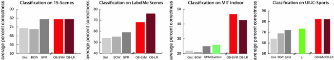
(Best viewed in colors and magnification) Comparison of classification performance of different features (GIST vs. BOW vs. SPM vs. object bank) and classifiers (SVM vs. LR) on (left to right) 15 scene, LabelMe, UIUC-Sports and MIT-Indoor datasets. In the LabelMe dataset, the ‘ideal’ classification accuracy is \(90\,\%\), where we use the human ground-truth object identities to predict the labels of the scene classes. Performance of previous related algorithms of the original dataset are displayed by using the green bars
The difference is not significant (\(1\,\%\)). One possible reason for this is that there is not much view variance in most of the object detector training data from ImageNet. Majority of the training images are front shots of the objects.
Fig. 8 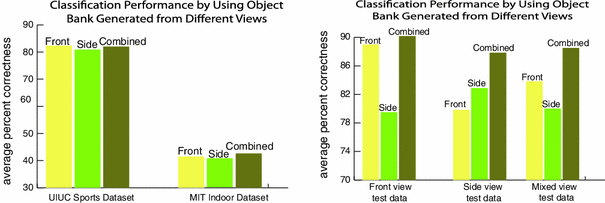
Left Classification performance of object bank generated from detectors trained on images with different view points on the UIUC sports dataset and the MIT Indoor dataset. Right Classification performance of object bank generated from different views on images with different view points
We use Gaussian kernel for smoothing the score.
Fig. 12 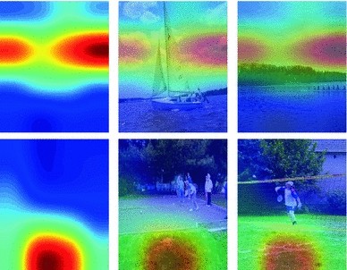
Left Heat map of possible locations estimated from classification performance of Object Bank representation generated from different spatial locations. Right Example images with the possible location map overlaid on the original image
The candidates are ‘sky’, ‘snow’, ‘water’, ‘building’, ‘rock’, ‘mountain’, ‘car’, ‘racquet’, ‘sail-boat’, ‘horse’, ‘human’, ‘boat’, ‘frame’, ‘snowboard’, ‘net’, ‘oar’, ‘wicket’, ‘helmet’, ‘mallet’, ‘window’, ‘cloud’, ‘court’, ‘tree’, ‘grass’, and ‘sand’.
racquet, helmet, window
The fastest feature extraction time of the available code evaluated is 7 s.


References
Bo, L., Ren, X., & Fox, D. (2011, December). Hierarchical matching pursuit for image classification: Architecture and fast algorithms. In Advances in neural information processing systems.
Bosch, A., Zisserman, A., & Munoz, X. (2006). Scene classification via pLSA. Proceedings of ECCV, 4, 517–530.
Bourdev, L., & Malik, J. (2009). Poselets: Body part detectors trained using 3D human pose annotations. In ICCV.
Csurka, G., Bray, C., Dance, C., & Fan, L. (2004). Visual categorization with bags of keypoints. In ECCV: Workshop on Statistical Learning in Computer Vision (pp. 1–22).
Dalal, N., & Triggs, B. (2005). Histograms of oriented gradients for human detection. In IEEE Computer Society Conference on Computer Vision and Pattern Recognition (Vol. 1, p. 886).
Deng, J., Dong, W., Socher, R., Li, L.-J., Li, K., & Fei-Fei, L. (2009). ImageNet: A large-scale hierarchical image database. In CVPR09 (p. 9).
Desai, C., Ramanan, D., & Fowlkes, C. (2009). Discriminative models for multi-class object layout. In IEEE 12th International Conference on Computer Vision (pp. 229–236). New York: IEEE.
Dixit, M., Rasiwasia, N., & Vasconcelos, N. (2011). Adapted Gaussian models for image classification. In CVPR.
Edition, B., & Sampler, BNC. British National Corpus.
Farhadi, A., Endres, I., & Hoiem, D. (2010). Attribute-centric recognition for cross-category generalization. In IEEE Conference on Computer Vision and Pattern Recognition (CVPR) (pp. 2352–2359). New York: IEEE.
Fei-Fei, L., & Perona, P. (2005). A Bayesian hierarchy model for learning natural scene categories. In Computer Vision and Pattern Recognition.
Fei-Fei, L., Fergus, R., & Perona, P. (2006). One-shot learning of object categories. In IEEE Transactions on Pattern Analysis and Machine Intelligence.
Fei-Fei, L., Fergus, R., & Torralba, A. (2007). Recognizing and learning object categories. Short course CVPR. Retrieved from http://people.csail.mit.edu/torralba/shortCourseRLOC/index.html.
Felzenszwalb, P., Girshick, R., McAllester, D., & Ramanan, D. (2007). Object detection with discriminatively trained part based models. Journal of Artificial Intelligence Research, 29.
Ferrari, V., & Zisserman, A. (2007). Learning visual attributes. In NIPS.
Von Ahn, L. (2006). Games with a purpose. Computer, 39(6), 92–94.
Freeman, W. T., & Adelson, E. H. (1991). The design and use of steerable filters. IEEE Transactions on Pattern Analysis and Machine Intelligence, 13(9), 891–906.
Gao, S., Tsang, I., & Chia, L. T. (2010). Kernel sparse representation for image classification and face recognition. In Computer Vision-ECCV (pp. 1–14). Berlin: Springer.
Gao, S., Chia, L. T., & Tsang, I. W. H. (2011). Multi-layer group sparse coding-for concurrent image classification and annotation. In IEEE Conference on Computer Vision and Pattern Recognition (CVPR) (pp. 2809–2816). New York: IEEE.
Gehler, P., & Nowozin, S. (2009). On feature combination for multiclass object classification. In IEEE 12th International Conference on Computer Vision (pp. 221–228). New York: IEEE.
Griffin, G., Holub, A., & Perona, P. (2007). Caltech-256 object category dataset.
Hauptmann, A., Yan, R., Lin, W., Christel, M., & Wactlar, H. (2007). Can high-level concepts fill the semantic gap in video retrieval? A case study with broadcast news. IEEE Transactions on Multimedia, 9(5), 958.
Hoiem, D., & Efros, A. A., & Hebert, M. (2006). Putting objects in perspective. In CVPR (p. 2)
Ide, N., & Macleod, C. (2001). The American National Corpus: A standardized resource of American English. In Proceedings of Corpus Linguistics 2001, Citeseer (pp. 274–280).
Jin, Y., & Geman, S. (2006). Context and hierarchy in a probabilistic image model. In CVPR.
Lampert, C. H., Nickisch, H., & Harmeling, S. (2009). Learning to detect unseen object classes by between-class attribute transfer. In CVPR.
Lazebnik, S., Schmid, C., & Ponce, J. (2006). Beyond bags of features: Spatial pyramid matching for recognizing natural scene categories. Urbana: Beckman Institute.
Leung, T., & Malik, J. (2001, June). Representing and recognizing the visual appearance of materials using three-dimensional textons. IJCV, 43(1), 29–44.
Li, L.-J., & Fei-Fei, L. (20007). What, where and who? Classifying events by scene and object recognition. In ICCV.
Li, L.-J., Socher, R., & Fei-Fei, L. (2009). Towards total scene understanding: Classification, annotation and segmentation in an automatic framework. In CVPR.
Li, L.-J., Su, H., Lim, Y., & Fei-Fei, L. (2010). Objects as attributes for scene classification. In (ECCV), Workshop on PaA.
Li, L.-J., Su, H., Xing, E., & Fei-Fei, L. (2010). Object bank: A high-level image representation for scene classification & semantic feature sparsification. In NIPS.
Lowe, D. (1999). Object recognition from local scale-invariant features. In ICCV.
Miller, G. A. (1995). WordNet: A lexical database for English. In Communications of the ACM.
Oliva, A., & Torralba, A. (2001). Modeling the shape of the scene: A holistic representation of the spatial envelope. In IJCV.
Pandey, M., & Lazebnik, S. (2011). Scene recognition and weakly supervised object localization with deformable part-based models. In IEEE International Conference on Computer Vision (ICCV) (pp. 1307–1314). New York: IEEE.
Perona, P., & Malik, J. (1990). Scale-space and edge detection using anisotropic diffusion. PAMI, 12(7), 629–639.
Perronnin, F., Sánchez, J., & Mensink, T. (2010). Improving the fisher kernel for large-scale image classification. Computer Vision-ECCV, 2010, 143–156.
Quattoni, A., & Torralba, A. (2009). Recognizing indoor scenes. In CVPR.
Russell, B. C., Torralba, A., Murphy, K. P., & Freeman, W. T. (2005). Labelme: A database and web-based tool for image, annotation.
Song, Z., Chen, Q., Huang, Z., Hua, Y., & Yan, S. (2011). Contextualizing object detection and classification. In IEEE Conference on Computer Vision and Pattern Recognition (CVPR).
Sudderth, E., Torralba, A., Freeman, W. T., & Willsky, A. (2005). Learning hierarchical models of scenes, objects, and parts. In Proceedings of International Conference on Computer Vision.
Torresani, L., Szummer, M., & Fitzgibbon, A. (2010). Efficient object category recognition using classemes. In ECCV.
Tu, Z., Chen, X., Yuille, A. L., & Zhu, S. C. (2005). Image parsing: Unifying segmentation, detection, and recognition. International Journal of Computer Vision, 63(2), 113–140.
Varma, M., & Zisserman, A. (2003). Texture classification: Are filter banks necessary? In CVPR03 (Vol. II, pp. 691–698).
Vogel, J., & Schiele, B. (2004). A semantic typicality measure for natural scene categorization. In DAGM’04 Annual Pattern Recognition Symposium, Tuebingen, Germany.
Wang, J., Yang, J., Yu, K., Lv, F., Huang, T., & Gong, Y. (2010). Locality-constrained linear coding for image classification. In IEEE Conference on Computer Vision and Pattern Recognition (CVPR) (pp. 3360–3367). New York: IEEE.
Zhu, L., Chen, Y., & Yuille, A. (2007). Unsupervised learning of a probabilistic grammar for object detection and parsing. Advances in neural information processing systems, 19, 1617.
Author information
Authors and Affiliations
Corresponding author
Rights and permissions
About this article
Cite this article
Li, LJ., Su, H., Lim, Y. et al. Object Bank: An Object-Level Image Representation for High-Level Visual Recognition. Int J Comput Vis 107, 20–39 (2014). https://doi.org/10.1007/s11263-013-0660-x
Received:
Accepted:
Published:
Issue Date:
DOI: https://doi.org/10.1007/s11263-013-0660-x