Selective Search for Object Recognition

Abstract

This paper addresses the problem of generating possible object locations for use in object recognition. We introduce selective search which combines the strength of both an exhaustive search and segmentation. Like segmentation, we use the image structure to guide our sampling process. Like exhaustive search, we aim to capture all possible object locations. Instead of a single technique to generate possible object locations, we diversify our search and use a variety of complementary image partitionings to deal with as many image conditions as possible. Our selective search results in a small set of data-driven, class-independent, high quality locations, yielding 99 % recall and a Mean Average Best Overlap of 0.879 at 10,097 locations. The reduced number of locations compared to an exhaustive search enables the use of stronger machine learning techniques and stronger appearance models for object recognition. In this paper we show that our selective search enables the use of the powerful Bag-of-Words model for recognition. The selective search software is made publicly available (Software: http://disi.unitn.it/~uijlings/SelectiveSearch.html).

1 Introduction

For a long time, objects were sought to be delineated before their identification. This gave rise to segmentation, which aims for a unique partitioning of the image through a generic algorithm, where there is one part for all object silhouettesin the image. Research on this topic has yielded tremendous progress over the past years ( Arbeláez et al. 2011; Comaniciu and Meer 2002; Felzenszwalb and Huttenlocher 2004; Shi and Malik 2000). But images are intrinsically hierarchical: In Fig. 1a the salad and spoons are inside the salad bowl, which in turn stands on the table. Furthermore, depending on the context the term table in this picture can refer to only the wood or include everything on the table. Therefore both the nature of images and the different uses of an object category are hierarchical. This prohibits the unique partitioning of objects for all but the most specific purposes. Hence for most tasks multiple scales in a segmentation are a necessity. This is most naturally addressed by using a hierarchical partitioning, as done for example by Arbeláez et al. (2011).

Fig. 1

There is a high variety of reasons that an image region forms an object. In (b) the cats can be distinguished by colour, not texture. In (c) the chameleon can be distinguished from the surrounding leaves by texture, not colour. In (d) the wheels can be part of the car because they are enclosed, not because they are similar in texture or colour. Therefore, to find objects in a structured way it is necessary to use a variety of diverse strategies. Furthermore, an image is intrinsically hierarchical as there is no single scale for which the complete table, salad bowl, and salad spoon can be found in (a)

Besides that a segmentation should be hierarchical, a generic solution for segmentation using a single strategy may not exist at all. There are many conflicting reasons why a region should be grouped together: In Fig. 1b the cats can be separated using colour, but their texture is the same. Conversely, in Fig. 1c the chameleon is similar to its surrounding leaves in terms of colour, yet its texture differs. Finally, in Fig. 1d, the wheels are wildly different from the car in terms of both colour and texture, yet are enclosed by the car. Individual visual features therefore cannot resolve the ambiguity of segmentation.

And, finally, there is a more fundamental problem. Regions with very different characteristics, such as a face over a sweater, can only be combined into one object after it has been established that the object at hand is a human. Hence without prior recognition it is hard to decide that a face and a sweater are part of one object ( Tu et al. 2005).

This has led to the opposite of the traditional approach: to do localisation through the identification of an object. This recent approach in object recognition has made enormous progress in less than a decade ( Dalal and Triggs 2005; Felzenszwalb et al. 2010; Harzallah et al. 2009; Viola and Jones 2001). With an appearance model learned from examples, an exhaustive search is performed where every location within the image is examined as to not miss any potential object location ( Dalal and Triggs 2005; Felzenszwalb et al. 2010; Harzallah et al. 2009; Viola and Jones 2001).

However, the exhaustive search itself has several drawbacks. Searching every possible location is computationally infeasible. The search space has to be reduced by using a regular grid, fixed scales, and fixed aspect ratios. In most cases the number of locations to visit remains huge, so much that alternative restrictions need to be imposed. The classifier is simplified and the appearance model needs to be fast. Furthermore, a uniform sampling yields many boxes for which it is immediately clear that they are not supportive of an object. Rather then sampling locations blindly using an exhaustive search, a key question is: Can we steer the sampling by a data-driven analysis?

In this paper, we aim to combine the best of the intuitions of segmentation and exhaustive search and propose a data-driven selective search. Inspired by bottom-up segmentation, we aim to exploit the structure of the image to generate object locations. Inspired by exhaustive search, we aim to capture all possible object locations. Therefore, instead of using a single sampling technique, we aim to diversify the sampling techniques to account for as many image conditions as possible. Specifically, we use a data-driven grouping-based strategy where we increase diversity by using a variety of complementary grouping criteria and a variety of complementary colour spaces with different invariance properties. The set of locations is obtained by combining the locations of these complementary partitionings. Our goal is to generate a class-independent, data-driven, selective search strategy that generates a small set of high-quality object locations.

Our application domain of selective search is object recognition. We therefore evaluate on the most commonly used dataset for this purpose, the Pascal VOC detection challenge which consists of 20 object classes. The size of this dataset yields computational constraints for our selective search. Furthermore, the use of this dataset means that the quality of locations is mainly evaluated in terms of bounding boxes. However, our selective search applies to regions as well and is also applicable to concepts such as “grass”.

In this paper we propose selective search for object recognition. Our main research questions are: (1) What are good diversification strategies for adapting segmentation as a selective search strategy? (2) How effective is selective search in creating a small set of high-quality locations within an image? (3) Can we use selective search to employ more powerful classifiers and appearance models for object recognition?

2 Related Work

We confine the related work to the domain of object recognition and divide it into three categories: Exhaustive search, segmentation, and other sampling strategies that do not fall in either category.

2.1 Exhaustive Search

As an object can be located at any position and scale in the image, it is natural to search everywhere ( Dalal and Triggs 2005; Harzallah et al. 2009; Viola and Jones 2004). However, the visual search space is huge, making an exhaustive search computationally expensive. This imposes constraints on the evaluation cost per location and/or the number of locations considered. Hence most of these sliding window techniques use a coarse search grid and fixed aspect ratios, using weak classifiers and economic image features such as HOG ( Dalal and Triggs 2005; Harzallah et al. 2009; Viola and Jones 2004). This method is often used as a preselection step in a cascade of classifiers ( Harzallah et al. 2009; Viola and Jones 2004).

Related to the sliding window technique is the highly successful part-based object localisation method of Felzenszwalb et al. (2010). Their method also performs an exhaustive search using a linear SVM and HOG features. However, they search for objects and object parts, whose combination results in an impressive object detection performance.

Lampert et al. (2009) proposed using the appearance model to guide the search. This both alleviates the constraints of using a regular grid, fixed scales, and fixed aspect ratio, while at the same time reduces the number of locations visited. This is done by directly searching for the optimal window within the image using a branch and bound technique. While they obtain impressive results for linear classifiers, Alexe et al. (2010) found that for non-linear classifiers the method in practice still visits over a 100,000 windows per image.

Instead of a blind exhaustive search or a branch and bound search, we propose selective search. We use the underlying image structure to generate object locations. In contrast to the discussed methods, this yields a completely class-independent set of locations. Furthermore, because we do not use a fixed aspect ratio, our method is not limited to objects but should be able to find stuff like “grass” and “sand” as well (this also holds for Lampert et al. (2009)). Finally, we hope to generate fewer locations, which should make the problem easier as the variability of samples becomes lower. And more importantly, it frees up computational power which can be used for stronger machine learning techniques and more powerful appearance models.

2.2 Segmentation

Both  Carreira and Sminchisescu (2010) and Endres and Hoiem (2010) propose to generate a set of class independent object hypotheses using segmentation. Both methods generate multiple foreground/background segmentations, learn to predict the likelihood that a foreground segment is a complete object, and use this to rank the segments. Both algorithms show a promising ability to accurately delineate objects within images, confirmed by Li et al. (2010) who achieve state-of-the-art results on pixel-wise image classification using Carreira and Sminchisescu (2010). As common in segmentation, both methods rely on a single strong algorithm for identifying good regions. They obtain a variety of locations by using many randomly initialised foreground and background seeds. In contrast, we explicitly deal with a variety of image conditions by using different grouping criteria and different representations. This means a lower computational investment as we do not have to invest in the single best segmentation strategy, such as using the excellent yet expensive contour detector of Arbeláez et al. (2011). Furthermore, as we deal with different image conditions separately, we expect our locations to have a more consistent quality. Finally, our selective search paradigm dictates that the most interesting question is not how our regions compare to Carreira and Sminchisescu (2010), Endres and Hoiem (2010), but rather how they can complement each other.

Gu et al. (2009) address the problem of carefully segmenting and recognizing objects based on their parts. They first generate a set of part hypotheses using a grouping method based on  Arbeláez et al. (2011). Each part hypothesis is described by both appearance and shape features. Then, an object is recognized and carefully delineated by using its parts, achieving good results for shape recognition. In their work, the segmentation is hierarchical and yields segments at all scales. However, they use a single grouping strategy whose power of discovering parts or objects is left unevaluated. In this work, we use multiple complementary strategies to deal with as many image conditions as possible. We include the locations generated using Arbeláez et al. (2011) in our evaluation.

2.3 Other Sampling Strategies

 Alexe et al. (2012) address the problem of the large sampling space of an exhaustive search by proposing to search for any object, independent of its class. In their method they train a classifier on the object windows of those objects which have a well-defined shape (as opposed to stuff like “grass” and “sand”). Then instead of a full exhaustive search they randomly sample boxes to which they apply their classifier. The boxes with the highest “objectness” measure serve as a set of object hypotheses. This set is then used to greatly reduce the number of windows evaluated by class-specific object detectors. We compare our method with their work.

Another strategy is to use visual words of the Bag-of-Words model to predict the object location. Vedaldi (2009) use jumping windows (Chum and ZissermanZ 2007), in which the relation between individual visual words and the object location is learned to predict the object location in new images. Maji and Malik (2009) combine multiple of these relations to predict the object location using a Hough-transform, after which they randomly sample windows close to the Hough maximum. In contrast to learning, we use the image structure to sample a set of class-independent object hypotheses.

To summarize, our novelty is as follows. Instead of an exhaustive search ( Dalal and Triggs 2005; Felzenszwalb et al. 2010; Harzallah et al. 2009; Viola and Jones 2004) we use segmentation as selective search yielding a small set of class independent object locations. In contrast to the segmentation of Carreira and Sminchisescu (2010), Endres and Hoiem (2010) instead of focusing on the best segmentation algorithm ( Arbeláez et al. 2011), we use a variety of strategies to deal with as many image conditions as possible, thereby severely reducing computational costs while potentially capturing more objects accurately. Instead of learning an objectness measure on randomly sampled boxes ( Alexe et al. 2012), we use a bottom-up grouping procedure to generate good object locations.

3 Selective Search

In this section we detail our selective search algorithm for object recognition and present a variety of diversification strategies to deal with as many image conditions as possible. A selective search algorithm is subject to the following design considerations:

• Capture All Scales. Objects can occur at any scale within the image. Furthermore, some objects have less clear boundaries then other objects. Therefore, in selective search all object scales have to be taken into account, as illustrated in Fig. 2. This is most naturally achieved by using an hierarchical algorithm.

  Fig. 2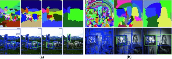

  

  Two examples of our selective search showing the necessity of different scales. On the left we find many objects at different scales. On the right we necessarily find the objects at different scales as the girl is contained by the tv

• Diversification. There is no single optimal strategy to group regions together. As observed earlier in Fig. 1, regions may form an object because of only colour, only texture, or because parts are enclosed. Furthermore, lighting conditions such as shading and the colour of the light may influence how regions form an object. Therefore instead of a single strategy which works well in most cases, we want to have a diverse set of strategies to deal with all cases.

• Fast to Compute. The goal of selective search is to yield a set of possible object locations for use in a practical object recognition framework. The creation of this set should not become a computational bottleneck, hence our algorithm should be reasonably fast.

3.1 Selective Search by Hierarchical Grouping

We take a hierarchical grouping algorithm to form the basis of our selective search. Bottom-up grouping is a popular approach to segmentation (Comaniciu and Meer 2002; Felzenszwalb and Huttenlocher 2004), hence we adapt it for selective search. Because the process of grouping itself is hierarchical, we can naturally generate locations at all scales by continuing the grouping process until the whole image becomes a single region. This satisfies the condition of capturing all scales.

As regions can yield richer information than pixels, we want to use region-based features whenever possible. To get a set of small starting regions which ideally do not span multiple objects, we use the fast method of  Felzenszwalb and Huttenlocher (2004), which Arbeláez et al. (2011) found well-suited for such purpose.

Our grouping procedure now works as follows. We first use (Felzenszwalb and Huttenlocher 2004) to create initial regions. Then we use a greedy algorithm to iteratively group regions together: First the similarities between all neighbouring regions are calculated. The two most similar regions are grouped together, and new similarities are calculated between the resulting region and its neighbours. The process of grouping the most similar regions is repeated until the whole image becomes a single region. The general method is detailed in Algorithm 1.

For the similarity $s(r_i, r_j)$ between region $r_i$ and $r_j$ we want a variety of complementary measures under the constraint that they are fast to compute. In effect, this means that the similarities should be based on features that can be propagated through the hierarchy, i.e. when merging region $r_i$ and $r_j$ into $r_t$, the features of region $r_t$ need to be calculated from the features of $r_i$ and $r_j$ without accessing the image pixels.

3.2 Diversification Strategies

The second design criterion for selective search is to diversify the sampling and create a set of complementary strategies whose locations are combined afterwards. We diversify our selective search (1) by using a variety of colour spaces with different invariance properties, (2) by using different similarity measures $s_{ij}$, and (3) by varying our starting regions.

Complementary Colour Spaces. We want to account for different scene and lighting conditions. Therefore we perform our hierarchical grouping algorithm in a variety of colour spaces with a range of invariance properties. Specifically, we the following colour spaces with an increasing degree of invariance: (1) $RGB$, (2) the intensity (grey-scale image) $I$, (3) $Lab$, (4) the $rg$ channels of normalized $RGB$ plus intensity denoted as $rgI$, (5) $HSV$, (6) normalized $RGB$ denoted as $rgb$, (7) $C$ Geusebroek et al. (2001) which is an opponent colour space where intensity is divided out, and finally (8) the Hue channel $H$ from $HSV$. The specific invariance properties are listed in Table 1.

Table 1 The invariance properties of both the individual colour channels and the colour spaces used in this paper, sorted by degree of invariance

Of course, for images that are black and white a change of colour space has little impact on the final outcome of the algorithm. For these images we rely on the other diversification methods for ensuring good object locations.

In this paper we always use a single colour space throughout the algorithm, meaning that both the initial grouping algorithm of Felzenszwalb and Huttenlocher (2004) and our subsequent grouping algorithm are performed in this colour space.

Complementary Similarity Measures. We define four complementary, fast-to-compute similarity measures. These measures are all in range $[0,1]$ which facilitates combinations of these measures.

• $s_{colour}(r_i,r_j)$ measures colour similarity. Specifically, for each region we obtain one-dimensional colour histograms for each colour channel using 25 bins, which we found to work well. This leads to a colour histogram $C_i = \{c_i^1, \cdots , c_i^n\}$ for each region $r_i$ with dimensionality $n=75$ when three colour channels are used. The colour histograms are normalised using the $L_1$ norm. Similarity is measured using the histogram intersection:

  $$\begin{aligned} s_{colour}(r_i, r_j) = \sum _{k=1}^{n} \min (c_i^k, c_j^k). \end{aligned}$$

  (1)

  The colour histograms can be efficiently propagated through the hierarchy by

  $$\begin{aligned} C_t = \frac{\text{ size }(r_i) \times C_i + \text{ size }(r_j) \times C_j}{\text{ size }(r_i) + \text{ size }(\text{ r }_\mathrm{j})}. \end{aligned}$$

  (2)

  The size of a resulting region is simply the sum of its constituents: $\text{ size }(r_t) = \text{ size }(r_i) + \text{ size }(r_j)$.

• $s_{texture}(r_i,r_j)$ measures texture similarity. We represent texture using fast SIFT-like measurements as SIFT itself works well for material recognition ( Liu et al. 2010). We take Gaussian derivatives in eight orientations using $\sigma =1$ for each colour channel. For each orientation for each colour channel we extract a histogram using a bin size of 10. This leads to a texture histogram $T_i = \{t_i^1, \cdots , t_i^n\}$ for each region $r_i$ with dimensionality $n=240$ when three colour channels are used. Texture histograms are normalised using the $L_1$ norm. Similarity is measured using histogram intersection:

  $$\begin{aligned} s_{texture}(r_i, r_j) = \sum _{k=1}^{n} \min (t_i^k, t_j^k). \end{aligned}$$

  (3)

  Texture histograms are efficiently propagated through the hierarchy in the same way as the colour histograms.

• $s_{size}(r_i,r_j)$ encourages small regions to merge early. This forces regions in $S$, i.e. regions which have not yet been merged, to be of similar sizes throughout the algorithm. This is desirable because it ensures that object locations at all scales are created at all parts of the image. For example, it prevents a single region from gobbling up all other regions one by one, yielding all scales only at the location of this growing region and nowhere else. $s_{size}(r_i, r_j)$ is defined as the fraction of the image that $r_i$ and $r_j$ jointly occupy:

  $$\begin{aligned} s_{size}(r_i,r_j) = 1 - \frac{\text{ size }(r_i) + \text{ size }(\text{ r }_\mathrm{j})}{\text{ size }({im})}, \end{aligned}$$

  (4)

  where $\text{ size }({im})$ denotes the size of the image in pixels.

• $s_{fill}(r_i,r_j)$ measures how well region $r_i$ and $r_j$ fit into each other. The idea is to fill gaps: if $r_i$ is contained in $r_j$ it is logical to merge these first in order to avoid any holes. On the other hand, if $r_i$ and $r_j$ are hardly touching each other they will likely form a strange region and should not be merged. To keep the measure fast, we use only the size of the regions and of the containing boxes. Specifically, we define $BB_{ij}$ to be the tight bounding box around $r_i$ and $r_j$. Now $s_{fill}(r_i,r_j)$ is the fraction of the image contained in $BB_{ij}$ which is not covered by the regions of $r_i$ and $r_j$:

  $$\begin{aligned} {fill}(r_i,r_j) = 1 - \frac{\text{ size }(BB_{ij}) - \text{ size }(r_i) - \text{ size }(r_i)}{\text{ size }({im})} \quad \quad \end{aligned}$$

  (5)

  We divide by $\text{ size }({im})$ for consistency with Eq.  4. Note that this measure can be efficiently calculated by keeping track of the bounding boxes around each region, as the bounding box around two regions can be easily derived from these.

In this paper, our final similarity measure is a combination of the above four:

$$\begin{aligned} s(r_i, r_j)&= a_1 s_{colour}(r_i, r_j) + a_2 s_{texture}(r_i, r_j) \nonumber \\&+a_3 s_{size}(r_i, r_j) + a_4 s_{fill}(r_i, r_j), \end{aligned}$$

(6)

where $a_i \in \{0,1\}$ denotes if the similarity measure is used or not. As we aim to diversify our strategies, we do not consider any weighted similarities.

Complementary Starting Regions. A third diversification strategy is varying the complementary starting regions. To the best of our knowledge, the method of Felzenszwalb and Huttenlocher (2004) is the fastest, publicly available algorithm that yields high quality starting locations. We could not find any other algorithm with similar computational efficiency so we use only this oversegmentation in this paper. But note that different starting regions are (already) obtained by varying the colour spaces, each which has different invariance properties. Additionally, we vary the threshold parameter $k$ in Felzenszwalb and Huttenlocher (2004).

3.3 Combining Locations

In this paper, we combine the object hypotheses of several variations of our hierarchical grouping algorithm. Ideally, we want to order the object hypotheses in such a way that the locations which are most likely to be an object come first. This enables one to find a good trade-off between the quality and quantity of the resulting object hypothesis set, depending on the computational efficiency of the subsequent feature extraction and classification method.

We choose to order the combined object hypotheses set based on the order in which the hypotheses were generated in each individual grouping strategy. However, as we combine results from up to 80 different strategies, such order would too heavily emphasize large regions. To prevent this, we include some randomness as follows. Given a grouping strategy $j$, let $r_i^j$ be the region which is created at position $i$ in the hierarchy, where $i=1$ represents the top of the hierarchy (whose corresponding region covers the complete image). We now calculate the position value $v_i^j$ as $\text{ RND } \times i$, where $\text{ RND }$ is a random number in range $[0,1]$. The final ranking is obtained by ordering the regions using $v_i^j$.

When we use locations in terms of bounding boxes, we first rank all the locations as detailed above. Only afterwards we filter out lower ranked duplicates. This ensures that duplicate boxes have a better chance of obtaining a high rank. This is desirable because if multiple grouping strategies suggest the same box location, it is likely to come from a visually coherent part of the image.

4 Object Recognition Using Selective Search

This paper uses the locations generated by our selective search for object recognition. This section details our framework for object recognition.

Two types of features are dominant in object recognition: histograms of oriented gradients (HOG) (Dalal and Triggs 2005) and bag-of-words ( Csurka et al. 2004; Sivic and Zisserman 2003). HOG has been shown to be successful in combination with the part-based model by  Felzenszwalb et al. (2010). However, as they use an exhaustive search, HOG features in combination with a linear classifier is the only feasible choice from a computational perspective. In contrast, our selective search enables the use of more expensive and potentially more powerful features. Therefore we use bag-of-words for object recognition ( Harzallah et al. 2009; Lampert et al. 2009; Vedaldi 2009). However, we use a more powerful (and expensive) implementation than (Harzallah et al. 2009; Lampert et al. 2009; Vedaldi 2009) by employing a variety of colour-SIFT descriptors ( van de Sande et al. 2010) and a finer spatial pyramid division ( Lazebnik et al. 2006).

Specifically we sample descriptors at each pixel on a single scale ($\sigma =1.2$). Using software from van de Sande et al. (2010), we extract SIFT ( Lowe 2004) and two colour SIFTs which were found to be the most sensitive for detecting image structures, Extended OpponentSIFT ( van de Sande et al. 2012) and RGB-SIFT ( van de Sande et al. 2010). We use a visual codebook of size 4,000 and a spatial pyramid with 4 levels using a $1 \times 1,\,2 \times 2,\,3 \times 3\,\mathrm{and}\,4 \times 4$ division. This gives a total feature vector length of 360,000. In image classification, features of this size are already used ( Perronnin et al. 2010; Zhou et al. 2010). Because a spatial pyramid results in a coarser spatial subdivision than the cells which make up a HOG descriptor, our features contain less information about the specific spatial layout of the object. Therefore, HOG is better suited for rigid objects and our features are better suited for deformable object types.

As classifier we employ a Support Vector Machine with a histogram intersection kernel using the Shogun Toolbox ( Sonnenburg et al. 2010). To apply the trained classifier, we use the fast, approximate classification strategy of  Maji et al. (2008), which was shown to work well for Bag-of-Words in Uijlings et al. (2010).

Our training procedure is illustrated in Fig. 3. The initial positive examples consist of all ground truth object windows. As initial negative examples we select from all object locations generated by our selective search that have an overlap of 20–50 % with a positive example. To avoid near-duplicate negative examples, a negative example is excluded if it has more than 70 % overlap with another negative. To keep the number of initial negatives per class below 20,000, we randomly drop half of the negatives for the classes car, cat, dog and person. Intuitively, this set of examples can be seen as difficult negatives which are close to the positive examples. This means they are close to the decision boundary and are therefore likely to become support vectors even when the complete set of negatives would be considered. Indeed, we found that this selection of training examples gives reasonably good initial classification models.

Fig. 3

The training procedure of our object recognition pipeline. As positive learning examples we use the ground truth. As negatives we use examples that have a 20–50 % overlap with the positive examples. We iteratively add hard negatives using a retraining phase

Then we enter a retraining phase to iteratively add hard negative examples (e.g. Felzenszwalb et al. (2010)): We apply the learned models to the training set using the locations generated by our selective search. For each negative image we add the highest scoring location. As our initial training set already yields good models, our models converge in only two iterations.

For the test set, the final model is applied to all locations generated by our selective search. The windows are sorted by classifier score while windows which have more than 30 % overlap with a higher scoring window are considered near-duplicates and are removed.

5 Evaluation

In this section we evaluate the quality of our selective search. We divide our experiments in four parts, each spanning a separate subsection:

• Diversification Strategies. We experiment with a variety of colour spaces, similarity measures, and thresholds of the initial regions, all which were detailed in Sect. 3.2. We seek a trade-off between the number of generated object hypotheses, computation time, and the quality of object locations. We do this in terms of bounding boxes. This results in a selection of complementary techniques which together serve as our final selective search method.

• Quality of Locations. We test the quality of the object location hypotheses resulting from the selective search.

• Object Recognition. We use the locations of our selective search in the Object Recognition framework detailed in Sect. 4. We evaluate performance on the Pascal VOC detection challenge.

• An upper bound of location quality. We investigate how well our object recognition framework performs when using an object hypothesis set of “perfect” quality. How does this compare to the locations that our selective search generates?

To evaluate the quality of our object hypotheses we define the Average Best Overlap (ABO) and Mean Average Best Overlap (MABO) scores, which slightly generalises the measure used in Endres and Hoiem (2010). To calculate the Average Best Overlap for a specific class $c$, we calculate the best overlap between each ground truth annotation $g_i^c \in G^c$ and the object hypotheses $L$ generated for the corresponding image, and average:

$$\begin{aligned} \text{ ABO } = \frac{1}{|G^c|} \sum _{g_i^c \in G^c} \max _{l_j \in L} \text{ Overlap }(g_i^c,l_j). \end{aligned}$$

(7)

The $\text{ Overlap }$ score is taken from Everingham et al. (2010) and measures the area of the intersection of two regions divided by its union:

$$\begin{aligned} \text{ Overlap }(g_i^c, l_j) = \frac{\text{ area }(g_i^c) \cap \text{ area }(\text{ l }_\mathrm{j})}{\text{ area }(g_i^c) \cup \text{ area }(\text{ l }_\mathrm{j})}. \end{aligned}$$

(8)

Analogously to Average Precision and Mean Average Precision, Mean Average Best Overlap is now defined as the mean ABO over all classes.

Other work often uses the recall derived from the Pascal Overlap Criterion to measure the quality of the boxes ( Alexe et al. 2010; Harzallah et al. 2009; Vedaldi 2009). This criterion considers an object to be found when the $\text{ Overlap }$ of Eq. 8 is larger than 0.5. However, in many of our experiments we obtain a recall between 95 and 100 % for most classes, making this measure too insensitive for this paper. However, we do report this measure when comparing with other work.

To avoid overfitting, we perform the diversification strategies experiments on the Pascal VOC 2007 train+val set. Other experiments are done on the Pascal VOC 2007 test set. Additionally, our object recognition system is benchmarked on the Pascal VOC 2010 detection challenge, using the independent evaluation server.

5.1 Diversification Strategies

In this section we evaluate a variety of strategies to obtain good quality object location hypotheses using a reasonable number of boxes computed within a reasonable amount of time.

5.1.1 Flat Versus Hierarchy

In the description of our method we claim that using a full hierarchy is more natural than using multiple flat partitionings by changing a threshold. In this section we test whether the use of a hierarchy also leads to better results. We therefore compare the use of Felzenszwalb and Huttenlocher (2004) with multiple thresholds against our proposed algorithm. Specifically, we perform both strategies in $RGB$ colour space. For Felzenszwalb and Huttenlocher (2004), we vary the threshold from $k=50$ to $k=1,000$ in steps of $50$. This range captures both small and large regions. Additionally, as a special type of threshold, we include the whole image as an object location because quite a few images contain a single large object only. Furthermore, we also take a coarser range from $k=50$ to $k=950$ in steps of $100$. For our algorithm, to create initial regions we use a threshold of $k=50$, ensuring that both strategies have an identical smallest scale. Additionally, as we generate fewer regions, we combine results using $k=50$ and $k=100$. As similarity measure $S$ we use the addition of all four similarities as defined in Eq. 6. Results are in Table 2.

Table 2 A comparison of multiple flat partitionings against hierarchical partitionings for generating box locations shows that for the hierarchical strategy the Mean Average Best Overlap (MABO) score is consistently higher at a similar number of locations

As can be seen, the quality of object hypotheses is better for our hierarchical strategy than for multiple flat partitionings: At a similar number of regions, our MABO score is consistently higher. Moreover, the increase in MABO achieved by combining the locations of two variants of our hierarchical grouping algorithm is much higher than the increase achieved by adding extra thresholds for the flat partitionings. We conclude that using all locations from a hierarchical grouping algorithm is not only more natural but also more effective than using multiple flat partitionings.

5.1.2 Individual Diversification Strategies

In this paper we propose three diversification strategies to obtain good quality object hypotheses: varying the colour space, varying the similarity measures, and varying the thresholds to obtain the starting regions. This section investigates the influence of each strategy. As basic settings we use the $RGB$ colour space, the combination of all four similarity measures, and threshold $k=50$. Each time we vary a single parameter. Results are given in Table 3.

Table 3 Mean Average Best Overlap for box-based object hypotheses using a variety of segmentation strategies

We start examining the combination of similarity measures on the left part of Table 3. Looking first at colour, texture, size, and fill individually, we see that the texture similarity performs worst with a MABO of 0.581, while the other measures range between 0.63 and 0.64. To test if the relatively low score of texture is due to our choice of feature, we also tried to represent texture by Local Binary Patterns Ojala et al. (2002). We experimented with 4 and 8 neighbours on different scales using different uniformity/consistency of the patterns (see Ojala et al. (2002)), where we concatenate LBP histograms of the individual colour channels. However, we obtained similar results (MABO of 0.577). We believe that one reason of the weakness of texture is because of object boundaries: When two segments are separated by an object boundary, both sides of this boundary will yield similar edge-responses, which inadvertently increases similarity.

While the texture similarity yields relatively few object locations, at 300 locations the other similarity measures still yield a MABO higher than 0.628. This suggests that when comparing individual strategies the final MABO scores in Table 3 are good indicators of trade-off between quality and quantity of the object hypotheses. Another observation is that combinations of similarity measures generally outperform the single measures. In fact, using all four similarity measures perform best yielding a MABO of 0.676.

Looking at variations in the colour space in the top-right of Table 3, we observe large differences in results, ranging from a MABO of 0.615 with 125 locations for the C colour space to a MABO of 0.693 with 463 locations for the HSV colour space. We note that Lab-space has a particularly good MABO score of 0.690 using only 328 boxes. Furthermore, the order of each hierarchy is effective: using the first 328 boxes of HSV colour space yields 0.690 MABO, while using the first 100 boxes yields 0.647 MABO. This shows that when comparing single strategies we can use only the MABO scores to represent the trade-off between quality and quantity of the object hypotheses set. We will use this in the next section when finding good combinations.

Experiments on the thresholds of Felzenszwalb and Huttenlocher (2004) to generate the starting regions show, in the bottom-right of Table 3, that a lower initial threshold results in a higher MABO using more object locations.

5.1.3 Combinations of Diversification Strategies

We combine object location hypotheses using a variety of complementary grouping strategies in order to get a good quality set of object locations. As a full search for the best combination is computationally expensive, we perform a greedy search using the MABO score only as optimization criterion. We have earlier observed that this score is representative for the trade-off between the number of locations and their quality.

From the resulting ordering we create three configurations: a single best strategy, a fast selective search, and a quality selective search using all combinations of individual components, i.e. colour space, similarities, thresholds, as detailed in Table 4. The greedy search emphasizes variation in the combination of similarity measures. This confirms our diversification hypothesis: In the quality version, next to the combination of all similarities, Fill and Size are taken separately. The remainder of this paper uses the three strategies in Table 4.

Table 4 Our selective search methods resulting from a greedy search

5.2 Quality of Locations

In this section we evaluate our selective search algorithms in terms of both Average Best Overlap and the number of locations on the Pascal VOC 2007 test set. We first evaluate box-based locations and afterwards briefly evaluate region-based locations.

5.2.1 Box-Based Locations

We compare with the sliding window search of Harzallah et al. (2009), the sliding window search of Felzenszwalb et al. (2010) using the window ratio’s of their models, the jumping windows of Vedaldi (2009), the “objectness” boxes of Alexe et al. (2012), the boxes around the hierarchical segmentation algorithm of Arbeláez et al. (2011), the boxes around the regions of Endres and Hoiem (2010), and the boxes around the regions of Carreira and Sminchisescu (2010). From these algorithms, only Arbeláez et al. (2011) is not designed for finding object locations. Yet Arbeláez et al. (2011) is one of the best contour detectors publicly available, and results in a natural hierarchy of regions. We include it in our evaluation to see if this algorithm designed for segmentation also performs well on finding good object locations. Furthermore, Carreira and Sminchisescu (2010); Endres and Hoiem (2010) are designed to find good object regions rather then boxes. Results are shown in Table 5 and Fig. 4.

Table 5 Comparison of recall, Mean Average Best Overlap (MABO) and number of window locations for a variety of methods on the Pascal 2007 test set

Fig. 4

Trade-off between quality and quantity of the object hypotheses in terms of bounding boxes on the Pascal 2007 test set. The dashed lines are for those methods whose quantity is expressed is the number of boxes per class. In terms of recall “Fast” selective search has the best trade-off. In terms of Mean Average Best Overlap the “Quality” selective search is comparable with Carreira and Sminchisescu (2010), Endres and Hoiem (2010) yet is much faster to compute and goes on longer resulting in a higher final MABO of 0.879

As shown in Table 5, our “Fast” and “Quality” selective search methods yield a close to optimal recall of 98 and 99 % respectively. In terms of MABO, we achieve 0.804 and 0.879 respectively. To appreciate what a Best Overlap of 0.879 means, Figure 5 shows for bike, cow, and person an example location which has an overlap score between 0.874 and 0.884. This illustrates that our selective search yields high quality object locations.

Fig. 5

Examples of locations for objects whose Best Overlap score is around our Mean Average Best Overlap of 0.879. The green boxes are the ground truth. The red boxes are created using the “Quality” selective search (Color figure online)

Furthermore, note that the standard deviation of our MABO scores is relatively low: 0.046 for the fast selective search, and 0.039 for the quality selective search. This shows that selective search is robust to difference in object properties, and also to image condition often related with specific objects (one example is indoor/outdoor lighting).

If we compare with other algorithms, the second highest recall is at 0.940 and is achieved by the jumping windows (Vedaldi 2009) using 10,000 boxes per class. As we do not have the exact boxes, we were unable to obtain the MABO score. This is followed by the exhaustive search of Felzenszwalb et al. (2010) which achieves a recall of 0.933 and a MABO of 0.829 at 100,352 boxes per class (this number is the average over all classes). This is significantly lower then our method while using at least a factor of 10 more object locations.

Note furthermore that the segmentation methods of Carreira and Sminchisescu (2010), Endres and Hoiem (2010) have a relatively high standard deviation. This illustrates that a single strategy can not work equally well for all classes. Instead, using multiple complementary strategies leads to more stable and reliable results.

If we compare the segmentation of Arbelaez Arbeláez et al. (2011) with a the single best strategy of our method, they achieve a recall of 0.752 and a MABO of 0.649 at 418 boxes, while we achieve 0.875 recall and 0.698 MABO using 286 boxes. This suggests that a good segmentation algorithm does not automatically result in good object locations in terms of bounding boxes.

Figure 4 explores the trade-off between the quality and quantity of the object hypotheses. In terms of recall, our “Fast” method outperforms all other methods. The method of Harzallah et al. (2009) seems competitive for the 200 locations they use, but in their method the number of boxes is per class while for our method the same boxes are used for all classes. In terms of MABO, both the object hypotheses generation method of Carreira and Sminchisescu (2010) and Endres and Hoiem (2010) have a good quantity/quality trade-off for the up to 790 object-box locations per image they generate. However, these algorithms are computationally 114 and 59 times more expensive than our “Fast” method.

Interestingly, the “objectness” method of Alexe et al. (2012) performs quite well in terms of recall, but much worse in terms of MABO. This is most likely caused by their non-maximum suppression, which suppresses windows which have more than an 0.5 overlap score with an existing, higher ranked window. And while this significantly improved results when a 0.5 overlap score is the definition of finding an object, for the general problem of finding the highest quality locations this strategy is less effective and can even be harmful by eliminating better locations.

Figure 6 shows for several methods the Average Best Overlap per class. It is derived that the exhaustive search of Felzenszwalb et al. (2010) which uses 10 times more locations which are class specific, performs similar to our method for the classes bike, table, chair, and sofa, for the other classes our method yields the best score. In general, the classes with the highest scores are cat, dog, horse, and sofa, which are easy largely because the instances in the dataset tend to be big. The classes with the lowest scores are bottle, person, and plant, which are difficult because instances tend to be small. Nevertheless, cow, sheep, and tv are not bigger than person and yet can be found quite well by our algorithm.

Fig. 6

The Average Best Overlap scores per class for several method for generating box-based object locations on Pascal VOC 2007 test. For all classes but table our “Quality” selective search yields the best locations. For 12 out of 20 classes our “Fast” selective search outperforms the expensive Carreira and Sminchisescu (2010); Endres and Hoiem (2010). We always outperform Alexe et al. (2012)

To summarize, selective search is very effective in finding a high quality set of object hypotheses using a limited number of boxes, where the quality is reasonable consistent over the object classes. The methods of Carreira and Sminchisescu (2010) and Endres and Hoiem (2010) have a similar quality/quantity trade-off for up to 790 object locations. However, they have more variation over the object classes. Furthermore, they are at least 59 and 13 times more expensive to compute for our “Fast” and “Quality” selective search methods respectively, which is a problem for current dataset sizes for object recognition. In general, we conclude that selective search yields the best quality locations at 0.879 MABO while using a reasonable number of 10,097 class-independent object locations.

5.2.2 Region-Based Locations

In this section we examine how well the regions that our selective search generates captures object locations. We do this on the segmentation part of the Pascal VOC 2007 test set. We compare with the segmentation of Arbeláez et al. (2011) and with the object hypothesis regions of both Carreira and Sminchisescu (2010); Endres and Hoiem (2010). Table 6 shows the results. Note that the number of regions is larger than the number of boxes as there are almost no exact duplicates.

Table 6 Comparison of algorithms to find a good set of potential object locations in terms of regions on the segmentation part of Pascal 2007 test

The object regions of both Carreira and Sminchisescu (2010); Endres and Hoiem (2010) are of similar quality as our “Fast” selective search, 0.665 MABO and 0.679 MABO respectively where our “Fast” search yields 0.666 MABO. While Carreira and Sminchisescu (2010); Endres and Hoiem (2010) use fewer regions these algorithms are respectively 114 and 59 times computationally more expensive. Our “Quality” selective search generates 22,491 regions and is respectively 25 and 13 times faster than Carreira and Sminchisescu (2010); Endres and Hoiem (2010), and has by far the highest score of 0.730 MABO.

Figure 7 shows the Average Best Overlap of the regions per class. For all classes except bike, our selective search consistently has relatively high ABO scores. The performance for bike is disproportionally lower for region-locations instead of object-locations, because bike is a wire-frame object and hence very difficult to accurately delineate.

Fig. 7

Comparison of the Average Best Overlap Scores per class between our method and others on the Pascal 2007 test set. Except for train, our “Quality” method consistently yields better Average Best Overlap scores

If we compare our method to others, the method of Endres and Hoiem (2010) is better for train, for the other classes our “Quality” method yields similar or better scores. For bird, boat, bus, chair, person, plant, and tv scores are 0.05 ABO better. For car we obtain 0.12 higher ABO and for bottle even 0.17 higher ABO. Looking at the variation in ABO scores in Table 6, we see that selective search has a slightly lower variation than the other methods: 0.093 MABO for “quality” and 0.108 for Endres and Hoiem (2010). However, this score is biased because of the wire-framed bicycle: without bicycle the difference becomes more apparent. The standard deviation for the “quality” selective search becomes 0.058, and 0.100 for Endres and Hoiem (2010). Again, this shows that by relying on multiple complementary strategies instead of a single strategy yields more stable results.

Figure 8 shows several example segmentations from our method and Carreira and Sminchisescu (2010), Endres and Hoiem (2010). In the first image, the other methods have problems keeping the white label of the bottle and the book apart. In our case, one of our strategies ignores colour while the “fill” similarity (Eq. 5) helps grouping the bottle and label together. The missing bottle part, which is dusty, is already merged with the table before this bottle segment is formed, hence “fill” will not help here. The second image is an example of a dark image on which our algorithm has generally strong results due to using a variety of colour spaces. In this particular image, the partially intensity invariant $Lab$ colour space helps to isolate the car. As we do not use the contour detection method of Arbeláez et al. (2011), our method sometimes generates segments with an irregular border, which is illustrated by the third image of a cat. The final image shows a very difficult example, for which only Carreira and Sminchisescu (2010) provides an accurate segment.

Fig. 8

A qualitative comparison of selective search, Carreira and Sminchisescu (2010), and Endres and Hoiem (2010). For our method we observe: ignoring colour allows finding the bottle, multiple colour spaces help in dark images (car), and not using Arbeláez et al. (2011) sometimes result in irregular borders such as the cat

Now because of the nature of selective search, rather than pitting methods against each other, it is more interesting to see how they can complement each other. As both Carreira and Sminchisescu (2010); Endres and Hoiem (2010) have a very different algorithm, the combination should prove effective according to our diversification hypothesis. Indeed, as can be seen in the lower part of Table 6, combination with our “Fast” selective search leads to 0.737 MABO at 6,438 locations. This is a higher MABO using less locations than our “quality” selective search. A combination of Carreira and Sminchisescu (2010); Endres and Hoiem (2010) with our “quality” sampling leads to 0.758 MABO at 25,355 locations. This is a good increase at only a modest extra number of locations.

To conclude, selective search is highly effective for generating object locations in terms of regions. The use of a variety of strategies makes it robust against various image conditions as well as the object class. The combination of Carreira and Sminchisescu (2010), Endres and Hoiem (2010) and our grouping algorithms into a single selective search showed promising improvements. Given these improvements, and given that there are many more different partitioning algorithms out there to use in a selective search, it will be interesting to see how far our selective search paradigm can still go in terms of computational efficiency, number of object locations, and the quality of object locations.

5.3 Object Recognition

In this section we will evaluate our selective search strategy for object recognition using the Pascal VOC 2010 detection task.

Our selective search strategy enables the use of expensive and powerful image representations and machine learning techniques. In this section we use selective search inside the Bag-of-Words based object recognition framework described in Sect. 4. The reduced number of object locations compared to an exhaustive search make it feasible to use such a strong Bag-of-Words implementation.

To give an indication of computational requirements: The pixel-wise extraction of three SIFT variants plus visual word assignment takes around 10 seconds and is done once per image. The final round of SVM learning takes around 8 hours per class on a GPU for approximately 30,000 training examples ( van de Sande et al. 2011) resulting from two rounds of mining negatives on Pascal VOC 2010. Mining hard negatives is done in parallel and takes around 11 h on 10 machines for a single round, which is around 40 s per image. This is divided into 30 s for counting visual word frequencies and 0.5 s per class for classification. Testing takes 40 s for extracting features, visual word assignment, and counting visual word frequencies, after which 0.5 s is needed per class for classification. For comparison, the code of Felzenszwalb et al. (2010) (without cascade, just like our version) needs for testing slightly less than 4 s per image per class. For the 20 Pascal classes this makes our framework faster during testing.

We evaluate results using the official evaluation server. This evaluation is independent as the test data has not been released. We compare with the top-4 of the competition. Note that while all methods in the top-4 are based on an exhaustive search using variations on part-based model of Felzenszwalb et al. (2010) with HOG-features, our method differs substantially by using selective search and Bag-of-Words features. Results are shown in Table 7.

Table 7 Results from the Pascal VOC 2010 detection task test set

It is shown that our method yields the best results for the classes plane, cat, cow, table, dog, plant, sheep, sofa, and tv. Except table, sofa, and tv, these classes are all non-rigid. This is expected, as Bag-of-Words is theoretically better suited for these classes than the HOG-features. Indeed, for the rigid classes bike, bottle, bus, car, person, and train the HOG-based methods perform better. The exception is the rigid class tv. This is presumably because our selective search performs well in locating tv’s, see Fig. 6.

In the Pascal 2011 challenge there are several entries wich achieve significantly higher scores than our entry. These methods use Bag-of-Words as additional information on the locations found by their part-based model, yielding better detection accuracy. Interestingly, however, by using Bag-of-Words to detect locations our method achieves a higher total recall for many classes ( Everingham et al. 2011).

Finally, our selective search enabled participation to the detection task of the ImageNet Large Scale Visual Recognition Challenge 2011 (ILSVRC2011) as shown in Table 8. This dataset contains 1,229,413 training images and 100,000 test images with 1,000 different object categories. Testing can be accelerated as features extracted from the locations of selective search can be reused for all classes. For example, using the fast Bag-of-Words framework of Uijlings et al. (2010), the time to extract SIFT-descriptors plus two colour variants takes 6.7 s and assignment to visual words takes 1.7 s ¹. Using a $1 \times 1, 2 \times 2, \mathrm{and}, 3 \times 3$ spatial pyramid division it takes 14 s to get all 172,032 dimensional features. Classification in a cascade on the pyramid levels then takes 0.3 s per class. For 1,000 classes, the total process then takes 323 s per image for testing. In contrast, using the part-based framework of  Felzenszwalb et al. (2010) it takes 3.9 s per class per image, resulting in 3,900 s per image for testing. This clearly shows that the reduced number of locations helps scaling towards more classes.

Table 8 Results for ImageNet Large Scale Visual Recognition Challenge 2011 (ILSVRC2011)

We conclude that compared to an exhaustive search, selective search enables the use of more expensive features and classifiers and scales better as the number of classes increase.

5.4 Pascal VOC 2012

Because the Pacal VOC 2012 is the latest and perhaps final VOC dataset, we briefly present results on this dataset to facilitate comparison with our work in the future. We present quality of boxes using the train+val set, the quality of segments on the segmentation part of train+val, and our localisation framework using a Spatial Pyramid of $1 \times 1, 2 \times 2, 3 \times 3, \mathrm{and}, 4 \times 4$ on the test set using the official evaluation server.

Results for the location quality are presented in Table 9. We see that for the box-locations the results are slightly higher than in Pascal VOC 2007. For the segments, however, results are worse. This is mainly because the 2012 segmentation set is considerably more difficult.

For the 2012 detection challenge, the Mean Average Precision is 0.350. This is similar to the 0.351 MAP obtained on Pascal VOC 2010.

Table 9 Quality of locations on Pascal VOC 2012 train+val

5.5 An Upper Bound of Location Quality

In this experiment we investigate how close our selective search locations are to the optimal locations in terms of recognition accuracy for Bag-of-Words features. We do this on the Pascal VOC 2007 test set.

The red line in Fig. 9 shows the MAP score of our object recognition system when the top $n$ boxes of our “quality” selective search method are used. The performance starts at 0.283 MAP using the first 500 object locations with a MABO of 0.758. It rapidly increases to 0.356 MAP using the first 3,000 object locations with a MABO of 0.855, and then ends at 0.360 MAP using all 10,097 object locations with a MABO of 0.883.

Fig. 9

Theoretical upper limit for the box selection within our object recognition framework. The red curve denotes the performance using the top $n$ locations of our “quality” selective search method, which has a MABO of 0.758 at 500 locations, 0.855 at 3,000 locations, and 0.883 at 10,000 locations. The magenta curve denotes the performance using the same top $n$ locations but now combined with the ground truth, which is the upper limit of location quality (MABO = 1). At 10,000 locations, our object hypothesis set is close to optimal in terms of object recognition accuracy (Color figure online)

The magenta line shows the performance of our object recognition system if we include the ground truth object locations to our hypotheses set, representing an object hypothesis set of “perfect” quality with a MABO score of 1. When only the ground truth boxes are used a MAP of 0.592 is achieved, which is an upper bound of our object recognition system. However, this score rapidly declines to 0.437 MAP using as few as 500 locations per image. Remarkably, when all 10,079 boxes are used the performance drops to 0.377 MAP, only 0.017 MAP more than when not including the ground truth. This shows that at 10,000 object locations our hypotheses set is close to what can be optimally achieved for our recognition framework. The most likely explanation is our use of SIFT, which is designed to be shift invariant Lowe (2004). This causes approximate boxes, of a quality visualised in Figure 5, to be still good enough. However, the small gap between the “perfect” object hypotheses set of 10,000 boxes and ours suggests that we arrived at the point where the degree of invariance for Bag-of-Words may have an adverse effect rather than an advantageous one.

The decrease of the “perfect” hypothesis set as the number of boxes becomes larger is due to the increased difficulty of the problem: more boxes means a higher variability, which makes the object recognition problem harder. Earlier we hypothesized that an exhaustive search examines all possible locations in the image, which makes the object recognition problem hard. To test if selective search alleviates the problem, we also applied our Bag-of-Words object recognition system on an exhaustive search, using the locations of Felzenszwalb et al. (2010). This results in a MAP of 0.336, while the MABO was 0.829 and the number of object locations 100,000 per class. The same MABO is obtained using 2,000 locations with selective search. At 2,000 locations, the object recognition accuracy is 0.347. This shows that selective search indeed makes the problem easier compared to exhaustive search by reducing the possible variation in locations.

To conclude, there is a trade-off between quality and quantity of object hypothesis and the object recognition accuracy. High quality object locations are necessary to recognise an object in the first place. Being able to sample fewer object hypotheses without sacrificing quality makes the classification problem easier and helps to improves results. Remarkably, at a reasonable 10,000 locations, our object hypothesis set is close to optimal for our Bag-of-Words recognition system. This suggests that our locations are of such quality that features with higher discriminative power than is normally found in Bag-of-Words are now required.

6 Conclusions

This paper proposed to adapt segmentation for selective search. We observed that an image is inherently hierarchical and that there are a large variety of reasons for a region to form an object. Therefore a single bottom-up grouping algorithm can never capture all possible object locations. To solve this we introduced selective search, where the main insight is to use a diverse set of complementary and hierarchical grouping strategies. This makes selective search stable, robust, and independent of the object-class, where object types range from rigid (e.g. car) to non-rigid (e.g. cat), and theoretically also to amorphous (e.g. water).

In terms of object windows, results show that our algorithm is superior to the “objectness” of Alexe et al. (2012) where our fast selective search reaches a quality of 0.804 Mean Average Best Overlap at 2,134 locations. Compared to Carreira and Sminchisescu (2010); Endres and Hoiem (2010), our algorithm has a similar trade-off between quality and quantity of generated windows with around 0.790 MABO for up to 790 locations, the maximum that they generate. Yet our algorithm is 13-59 times faster. Additionally, it creates up to 10,097 locations per image yielding a MABO as high as 0.879.

In terms of object regions, a combination of our algorithm with Carreira and Sminchisescu (2010); Endres and Hoiem (2010) yields a considerable jump in quality (MABO increases from 0.730 to 0.758), which shows that by following our diversification paradigm there is still room for improvement.

Finally, we showed that selective search can be successfully used to create a good Bag-of-Words based localisation and recognition system. In fact, we showed that the quality of our selective search locations are close to optimal for our version of Bag-of-Words based object recognition.

References

Alexe, B., Deselaers, T., Ferrari, V. (2010). What is an object? In CVPR.
Alexe, B., Deselaers, T., & Ferrari, V. (2012). Measuring the objectness of image windows. IEEE Transactions on Pattern Analysis and Machine Intelligence, 34(11), 2189–2202.
Arbeláez, P., Maire, M., Fowlkes, C., & Malik, J. (2011). Contour detection and hierarchical image segmentation. IEEE Transactions on Pattern Analysis and Machine Intelligence, 33(5), 898–916.
Carreira, J., Sminchisescu, C. (2010). Constrained parametric min-cuts for automatic object segmentation. In CVPR.
Chum, O., Zisserman, A. (2007). An exemplar model for learning object classes. In CVPR.
Comaniciu, D., & Meer, P. (2002). Mean shift: A robust approach toward feature space analysis. IEEE Transactions on Pattern Analysis and Machine Intelligence, 24, 603–619.
Csurka, G., Dance, C. R., Fan, L., Willamowski, J., & Bray, C. (2004). In ECCV statistical learning in computer vision: Visual categorization with bags of keypoints.
Dalal, N., Triggs, B. (2005). Histograms of oriented gradients for human detection. In CVPR.
Endres, I., Hoiem, D. (2010). Category independent object proposals. In ECCV.
Everingham, M., Gool, L. V., Williams, C., Winn, J., & Zisserman, A. (2011). The Pascal visual object classes challenge workshop: Overview and results of the detection challenge.
Everingham, M., van Gool, L., Williams, C. K. I., Winn, J., & Zisserman, A. (2010). The Pascal visual object classes (voc) challenge. International Journal of Computer Vision, 88, 303–338.
Felzenszwalb, P. F., Girshick, R. B., McAllester, D., & Ramanan, D. (2010). Object detection with discriminatively trained part based models. IEEE Transactions on Pattern Analysis and Machine Intelligence, 32, 1627–1645.
Felzenszwalb, P. F., & Huttenlocher, D. P. (2004). Efficient graph-based image segmentation. International Journal of Computer Vision, 59, 167–181.
Geusebroek, J. M., van den Boomgaard, R., Smeulders, A. W. M., & Geerts, H. (2001). Color invariance. IEEE Transactions on Pattern Analysis and Machine Intelligence, 23, 1338–1350.
Gu, C., Lim, J. J., Arbeláez, P., & Malik, J. (2009). In CVPR: Recognition using regions.
Harzallah, H., Jurie, F., & Schmid, C. (2009). In ICCV: Combining efficient object localization and image classification.
Lampert, C. H., Blaschko, M. B., & Hofmann, T. (2009). Efficient subwindow search: A branch and bound framework for object localization. IEEE Transactions on Pattern Analysis and Machine Intelligence, 31, 2129–2142.
Lazebnik, S., Schmid, C., Ponce, J. (2006). Beyond bags of features: Spatial pyramid matching for recognizing natural scene categories. In CVPR.
Li, F., & Carreira, J., Sminchisescu, C. (2010). In CVPR: Object recognition as ranking holistic figure-ground hypotheses.
Liu, C., Sharan, L., Adelson, E.H., Rosenholtz, R. (2010). Exploring features in a bayesian framework for material recognition. In Computer vision and pattern recognition 2010. IEEE.
Lowe, D. G. (2004). Distinctive image features from scale-invariant keypoints. International Journal of Computer Vision, 60, 91–110.
Maji, S., Berg, A. C., & Malik, J. (2008). In CVPR: Classification using intersection kernel support vector machines is efficient.
Maji, S., & Malik, J. (2009). Object detection using a max-margin hough transform. In CVPR.
Ojala, T., Pietikainen, M., & Maenpaa, T. (2002). Multiresolution gray-scale and rotation invariant texture classification with local binary patterns. IEEE Transactions on Pattern Analysis and Machine Intelligence, 24(7), 971–987.
Perronnin, F., Sánchez, J., & Thomas M. (2010). In ECCV: Improving the Fisher Kernel for large-scale image classification.
Shi, J., & Malik, J. (2000). Normalized cuts and image segmentation. IEEE Transactions on Pattern Analysis and Machine Intelligence, 22, 888–905.
Sivic, J., Zisserman, A.(2003). Video google: A text retrieval approach to object matching in videos. In ICCV.
Sonnenburg, S., Raetsch, G., Henschel, S., Widmer, C., Behr, J., Zien, A., et al. (2010). The shogun machine learning toolbox. Journal of Machine Learning Research, 11, 1799–1802.
Tu, Z., Chen, X., Yuille, A. L., & Zhu, S. (2005). Image parsing: Unifying segmentation, detection and recognition. Marr Prize Issue. International Journal of Computer Vision.
Uijlings, J. R. R., Smeulders, A. W. M., & Scha, R. J. H. (2010). Real-time visual concept classification. IEEE Transactions on Multimedia, 12(7), 665–681.
van de Sande, K. E. A., & Gevers, T. (2012). Illumination-invariant descriptors for discriminative visual object categorization. Technical report : University of Amsterdam.
van de Sande, K. E. A., Gevers, T., & Snoek, C. G. M. (2010). Evaluating color descriptors for object and scene recognition. IEEE Transactions on Pattern Analysis and Machine Intelligence, 32, 1582–1596.
van de Sande, K. E. A., Gevers, T., & Snoek, C. G. M. (2011). Empowering visual categorization with the GPU. IEEE Transactions on Multimedia, 13(1), 60–70.
Vedaldi, A., Gulshan, V., Varma, M., & Zisserman, A. (2009). In ICCV: Multiple kernels for object detection.
Viola, P., & Jones, M. (2001). Rapid object detection using a boosted cascade of simple features. In CVPR, Volume 1, 511–518.
Viola, P., & Jones, M. J. (2004). Robust real-time face detection. International Journal of Computer Vision, 57, 137–154.
Zhou, X., Kai, Y., Zhang, T., & Huang, T. S. (2010). In ECCV: Image classification using super-vector coding of local image descriptors.
Zhu, L., Chen, Y., Yuille, A., & Freeman, W. (2010). In CVPR: Latent hierarchical structural learning for object detection.
Author information
Authors and Affiliations
Corresponding author
Rights and permissions
About this article
Cite this article
Uijlings, J.R.R., van de Sande, K.E.A., Gevers, T. et al. Selective Search for Object Recognition. Int J Comput Vis 104, 154–171 (2013). https://doi.org/10.1007/s11263-013-0620-5
Received:
Accepted:
Published:
Issue Date:
DOI: https://doi.org/10.1007/s11263-013-0620-5