
Abstract
This article describes the mechanism of precursor events; the mechanism was determined through an experiment and simulation by considering non-uniform normal loading. In the experiment, real-time observations of a contact zone were performed using a longitudinal line contact of PMMA specimens (i.e., a slider on a stationary base block) under a total normal load of 400 N. Partial propagations of the detachment front were considered as precursor events, and it was found that non-uniform normal loading influences the occurrence frequency of the precursor events and the increasing rate of the propagation length. In the simulation, the time evolution of a multi-degree-of-freedom system with Coulomb friction was studied. The model considered in the simulation comprised multiple masses serially connected by linear springs on a stationary rigid plane. By regarding the precursor in the experiment to correspond to a partial slip (i.e., simultaneous slip of some of the masses) in the simulation, the influence of non-uniform normal loading on the precursor events can be explained to a certain extent. Additionally, it was found that the apparent static friction coefficient (i.e., the ratio of the maximum tangential load to the total normal load) could be lesser than the real static friction coefficient due to the residual strain in the slider.
1 Introduction
A sliding system shows various types of dynamic behaviors under different conditions. In particular, the repetitive occurrence of stick and slip phases (i.e., stick–slip) has attracted considerable attention as an interesting phenomenon in various fields such as vibration engineering [1–3], earthquake mechanics [4–9], and tribology [10, 11].
It has been known that stick–slip is caused by the difference between the static and kinetic friction, and it tends to appear at high contact loads and low driving speeds. A number of theoretical expressions have been proposed for describing the critical conditions for stick–slip in simple sliding systems [12–15]; they can be used to design robust-stable sliding systems. However, the mechanism of stick–slip remains to be elucidated; it is still not easy to precisely predict the onset of a global slip in sliding systems (e.g., earthquakes and mechanical clutches).
Recently, a number of studies have been carried out to clarify the initiation process of a global slip. In dry friction, it has been known that an interface crack propagates across a contact zone at the moment of transition from the stick to the slip phase [5, 16–21]. For example, Ohnaka and Kuwahara [5] elucidated the dynamic process of fracture propagation in a laboratory experiment using rock samples. In their experiment, quasi-static nucleation of fractures occurred in a weak region against shear stress with a growth rate of 10−2 m/s. Subsequently, an interface crack propagated and accelerated spontaneously with a speed of 103 m/s until a global slip was initiated.
Another similar example is the study of Rubinstein et al. [19, 20], who performed real-time measurements of the spatial and temporal changes in the contact zone between two polymethyl methacrylate (PMMA) blocks; they found three types of crack-like fronts with different speeds at the onset of a global slip. Besides, prior to the transition from the stick to the slip phase, they found a discrete sequence of rapid crack-like fronts propagating partially in the contact zone (precursors) [21]. It is believed that the elucidation of precursor events can help us predict (and hopefully control) the onset time and magnitude of the subsequent global slip.
This article describes the mechanism of precursor events; the mechanism was determined through an experiment and simulation by considering non-uniform normal loading. In the experiment, real-time observations of a contact zone were performed using a longitudinal line contact formed between a PMMA slider and a PMMA stationary base block under a total normal load of 400 N. Partial propagations of the detachment front were observed as precursor events, and it was found that non-uniform normal loading influenced the occurrence frequency of the precursor events and the increasing rate of the propagation length. In the simulation, the time evolution of a multi-degree-of-freedom system with Coulomb friction was studied. The model considered in the simulation comprised multiple masses serially connected by linear springs on a stationary rigid plane, which is similar to the train model proposed by Braun et al. [22] for a description of dynamics of crack-like processes. By regarding the precursor in the experiment to correspond to partial slip (i.e., simultaneous slip of some of the masses) in the simulation, the influence of non-uniform normal loading on the precursor events can be explained to a certain extent.
2 Experimental Details
2.1 Specimens
Two transparent blocks made of PMMA (Young’s modulus 2.5 GPa) were used as specimens to form a visible contact zone. Two rectangular blocks were used as the base and slider; the base had a length (X), width (Y), and height (Z) of 120, 30, and 40 mm, respectively, while the sliders dimensions were 100 mm (X), 5 mm (Y), and 20 mm (Z). The bottom edges of the slider were cut off along the longitudinal direction (X), resulting in the edges having an apex angle of 158°. Consequently, a longitudinal line contact directed along X was formed between the top surface of the base block and the bottom surface of the slider, which is apparently different from the study of Rubinstein et al. [19–21] using a plane contact between two acrylic blocks under a higher normal load (e.g., 4.5 kN). It should be noted that a unidirectional roughness of 5 μm rms was provided to both the contact surfaces by polishing in the Y direction with sandpaper.
2.2 Apparatus
A schematic diagram of the apparatus is shown in Fig. 1. There was an X-directional longitudinal line contact between the specimens (i.e., between the base block and slider).
The base block is mounted on its holder to firmly fix it, and a motorized stage that moves along the Z-axis (hereafter referred to as Z-directional motorized stage) is used to apply a force in the Z direction (i.e., the total normal load F Z ) to the slider via an elastic block made of silicon rubber (Young’s modulus 0.2 MPa and Poisson’s ratio 0.5) that easily deforms in the X direction with high stiction; thus, there is no relative motion at the top and bottom surfaces of the elastic block during the measurements. A tilt stage is used to change the angle of a lateral beam that holds two load cells that measure the force in the Z direction (hereafter referred to as Z-directional load cells); changing the angle induces non-uniform compression in the elastic block on the slider and leads to non-uniform loading of the line contact. The two load cells monitor the forces in the Z direction; they are separated by 60 mm and are positioned along a line in the X direction. A motorized stage that can move in the X direction (hereafter referred to as X-directional motorized stage) is used to apply a force directed in the X direction (i.e., the tangential load F X ) to the slider using the compliance of a load cell (effective stiffness: K = 0.8 MN/m) that measures the force in the X direction (hereafter referred to as X-directional load cell), to induce a series of transitions between the stick and the slip phases.
The X-directional load cell measures F X , and the two Z-directional load cells measure F ZA and F ZB , where F ZA denotes the partial normal load measured by the Z-directional load cell closer to the X-directional load cell, and F ZB denotes the partial normal load measured by the other Z-directional load cell. It is to be noted that the total normal load is given by F Z = F ZA + F ZB , and the difference between F ZA and F ZB represents the degree of non-uniformity of the normal loading.
The apparatus has a transmissive optical system that is used to observe the longitudinal contact zone between the transparent PMMA specimens. The contact zone is illuminated by a collimated laser sheet (X 120 mm; Y 3 mm) from a green laser diode (wavelength 532 nm). The incident angle to the contact zone is 65°, which is greater than the critical angle for the total reflection at a PMMA–air interface (42°); thus, an incident light that illuminates a real contact region is transmitted through the PMMA–PMMA interface, and an incident light that illuminates a non-contact region is reflected at the PMMA–air interface [19–21]. A high-speed camera captures line images of the contact zone using the transmitted light at frame rates of up to 250 kHz.
2.3 Procedure
The specimens were washed using detergent, water, and ethanol, and they were dried naturally. Subsequently, they were installed in the apparatus. A total normal load (F Z ) of up to 400 N was applied using the Z-directional motorized stage. By applying the normal load, the line contact zone was formed between the base block and slider with a length of 100 mm and a width of 0.8 mm; thus, the mean pressure for F Z = 400 N is estimated to be 5 MPa, which is eventually similar to the value in the study of Rubinstein et al. [19–21]. After waiting for a scheduled period, the tangential load (F X ) was increased from 0 N by moving the X-directional motorized stage in the positive X direction with a constant driving speed V of 0.1 mm/s. The time evolutions of F X , F ZA , and F ZB were recorded using a data logger at a sampling frequency of 1 kHz. Simultaneously, the images of the contact zone were captured using the high-speed camera at a frame rate of 1 kHz. It is to be noted that a single captured image consisted of 1280 pixels and had dimensions of 128 mm and 0.2 mm in the X and Y directions, respectively. Further, the intensity of a single pixel was represented using 256 shades of gray. All measurements were performed in an air-conditioned room, where the temperature and relative humidity were approximately 25 °C and 30%, respectively.
3 Experimental Results
3.1 Intensity of Transmitted Light and Real Contact Area
To establish the relationship between the intensity of the transmitted light and the real contact area, the contact characteristics of the two PMMA specimens were investigated; after capturing an image of the contact zone in stationary contact (i.e., F X = 0) under uniform loading (i.e., F ZA = F ZB ), the sum of intensities (i.e., the total intensity) of the pixels in the image was calculated.
A relaxation process was found in the temporal change of the total intensity (Fig. 2); the total intensity gradually increases and approaches to an asymptotic value under a normal loading condition. Consequently, we used an exponential decay function as the fitting curve, although there are a number of studies that reported the effect of the waiting time on the real contact area (i.e., the aging effect) proceeds via a logarithmic dependence in time [9, 23]. By carrying out curve-fitting analysis using the exponential decay function, we estimated the relaxation time to be approximately 200 s, and this value was independent of F Z (=200 or 400 N). This relaxation process probably resulted from the viscoelasticity and plasticity of PMMA; the growth of the real contact area takes a finite time since the external force (F Z ) on the slider should be balanced by the force generated by the deformation of contact asperities. It is to be noted that the mean pressure (5 MPa) is one or two orders of magnitude smaller than the yield stress of PMMA (i.e., approximately 100 MPa at 25 °C [24]).

Temporal change in the total intensity of the transmitted light for F Z = 400 N (F ZA = F ZB = 200 N) and 200 N (F ZA = F ZB = 100 N)
The total intensity at 1000 s shows a linear relationship with F Z (Fig. 3). This provides experimental confirmation that the real contact area can be qualitatively estimated using the total intensity of the transmitted light.

Dependence of the total intensity of transmitted light at 1000 s on the total normal load F Z under uniform loading (F ZA = F ZB )
3.2 Precursor Events
3.2.1 Precursor Events Under Uniform Loading
Experimental results pertaining to precursor events under uniform loading (F ZA = F ZB = 200 N) are shown in Fig. 4. The top graph shows the time evolution of the tangential load (F X ), the middle graph shows images of the time evolution of the longitudinal contact zone, and the bottom graph shows the time evolution of the total intensity. It is to be noted that the origin of the ordinate of the middle graph represents the initial position of the trailing edge of the slider; F X was applied in the positive direction at the position 0 mm.

Time evolutions of the tangential load F X and a magnified view around the first transition from the stick to the slip phase (top graph and inset), an image of the longitudinal contact zone (middle graph), and the total intensity of the transmitted light (bottom graph) under uniform loading. F ZA = F ZB = 200 N (F Z = 400 N); K = 0.8 MN/m; V = 0.1 mm/s; sampling frequency of the data logger: 1 kHz; frame rate of the high-speed camera: 1 kHz; vertical broken line: the first global slip
Focusing on the general behavior, we can find a periodic stick–slip with a sawtooth wave in the top graph. Starting from the origin, F X increases linearly for a constant loading rate (KV = 80 N/s) during the first stick phase. It then decreases sharply from approximately 200 N at the time marked by a vertical broken line; this decrease signifies the first global slip. Later in the graph, a linear increase and a sharp decrease in F X are observed. From the observation made at a higher sampling rate, the period of a single slip phase was determined to be approximately 2 ms for the condition employed in this study.
During the first stick phase, a number of small vertical drops are found in the top graph; some of them are magnified and indicated by arrows in the inset. They are precursor events observed before the global slip. In the middle graph, the precursor events are visualized as a series of discrete vertical lines that extend from the trailing edge (i.e., 0 mm) toward the leading edge (i.e., 100 mm) but do not reach the leading edge. The length of the vertical lines (i.e., the propagation length of precursors) increases with each event, and eventually it reaches the leading edge at the onset of the global slip. The growth property of the propagation length of the precursors is quite similar to the result in the study of Rubinstein et al. [21]; the propagation length of precursors increases linearly with time until the rapid growth occurs just prior to the first global slip. It should be noted that a number of precursors can be found even during the stick phase in the subsequent periods.
From the onset of the precursors, the total intensity gradually decreases by nearly 30% (shown in the bottom graph). The gradual decrease of the total intensity results from the non-uniformity of the real contact area caused by the occurrence of the precursors. It is possible that the slight quantitative difference of the decrement value of the total intensity between this study and the study of Rubinstein results from the shape of the slider. On the other hand, the sharp decrease in the total intensity during every precursor event implies that the essence of the precursor events is the decrease in the real contact area (i.e., the propagation of the detachment front [19–21]). An asymptotic increase in the total intensity after a precursor event shows the recovery of the real contact area during a stick phase. It is to be noted that this temporal change in the total intensity is the sum of the changes at various positions. A study of the time evolution of the total intensity at various positions (Fig. 5) shows that early precursor events occur close to the trailing edge and the region of precursor events extends toward the leading edge after every event.

Time evolutions of the total intensity of transmitted light at various positions. F ZA = F ZB = 200 N (F Z = 400 N); K = 0.8 MN/m; V = 0.1 mm/s; sampling frequency of the data logger: 1 kHz; frame rate of the high-speed camera: 1 kHz; vertical broken line: the first global slip
3.2.2 Precursor Events Under Non-Uniform Loading
The general features of precursor events under non-uniform loading are similar to those under uniform loading, but there is a clear difference (Figs. 6, 7). Non-uniform loading conditions with a higher load at the trailing edge relative to that at the leading edge (i.e., F ZA > F ZB ) result in a smaller number of precursor events than that under uniform loading conditions (i.e., F ZA = F ZB ); non-uniform loading conditions with a higher load at the leading edge (i.e., F ZA < F ZB ) lead to a larger number of precursor events relative to that in uniform loading conditions. Additionally, non-uniform normal loading affects the increasing rate of the propagation length of precursors. When F ZA > F ZB (Fig. 6), after a long incubation period, the propagation length of precursors increases significantly after each event; in contrast, when F ZA < F ZB (Fig. 7), after a short incubation period, the propagation length of precursors increases moderately after each event.

Time evolutions of the tangential load F X and a magnified view around the first transition from the stick to the slip phase (top graph and inset), an image of the longitudinal contact zone (middle graph), and the total intensity of transmitted light (bottom graph) under non-uniform loading. F ZA = 300 N; F ZB = 100 N (F Z = 400 N); K = 0.8 MN/m; V = 0.1 mm/s; sampling frequency of the data logger: 1 kHz; frame rate of the high-speed camera: 1 kHz; vertical broken line: the first global slip

Time evolutions of the tangential load F X and a magnified view around the first transition from the stick to the slip phase (top graph and inset), an image of the longitudinal contact zone (middle graph), and the total intensity of transmitted light (bottom graph) under non-uniform loading. F ZA = 100 N; F ZB = 300 N (F Z = 400 N); K = 0.8 MN/m; V = 0.1 mm/s; sampling frequency of the data logger: 1 kHz; frame rate of the high-speed camera: 1 kHz; vertical broken line: the first global slip
These effects are summarized in Fig. 8, which represents the relationship between the propagation length (L p) of precursors and the tangential load (F X ). It is to be noted that the number of symbols implies the number of observed precursor events (including one global slip); for the number of solid circles (F ZA > F ZB ), dotted circles (F ZA = F ZB ), and open circles (F ZA < F ZB ) are 11, 19, and 27, respectively. It is to be noted that the value of F X at the global slip is independent of the type of normal loading. This means that the value of the apparent static friction coefficient given by
is invariant (μsapp = 0.49) for the above-mentioned three conditions, where F Xmax denotes the maximum value of F X , which is observed at the first global slip.

Relationship between the propagation length L P of precursors and the tangential load F X under different loading conditions. L: length of the longitudinal line contact (=100 mm); dotted circle: uniform loading (F ZA = F ZB = 200 N); solid circle: non-uniform loading (F ZA = 300 N and F ZB = 100 N); and open circle: uniform loading (F ZA = 100 N and F ZB = 300 N)
4 Numerical Simulations
4.1 Analytical Model
Numerical simulations were performed with a simple physical model (Fig. 9) that considers multiple masses serially connected by linear springs on a stationary rigid plane. This model consists of two sections: a loading and a material sections. The loading section consists of an external point (labeled P) that moves with a constant speed V and a spring with a stiffness K that couples point P to the first block of the material section. The material section consists of N blocks with an identical mass m coupled to adjacent masses by identical springs, each with a stiffness k. The normal loads distributed to the blocks are not necessarily identical (e.g., Eq. 7). Friction f i acts on the contact between the ith block and the stationary plane under a normal load of w i .

Analytical model of the sliding system
4.2 Governing Equations
4.2.1 Equations of Motion
On the basis of the analytical model (Fig. 9), the equations of motion for the ith block are as follows:
where x i denotes the position of the ith block relative to its initial position, (•) represents the derivative with respect to time t, and F X denotes the tangential load given by
Friction f i that acts on the contact of the ith block is given by
The static friction \( f_{\text{s}}^{(i)} \) is determined by considering the static force balance (under \( \dot{x}_{i} = 0 \)) and takes a value in the following range:
where \( f_{\text{smax}}^{(i)} \) is the maximum static friction and μs is the static friction coefficient. On the other hand, using the kinetic friction coefficient μk, the kinetic friction \( f_{\text{k}}^{(i)} \) is given by
To analyze the precursor events using the simplest description of the friction coefficients, we employed the Coulomb friction model (i.e., μs = const., μk = const., and μs > μ k) in contrast to a more complex model of Braun et al. [22].
4.2.2 Method
The Runge–Kutta method was used to solve the governing equations numerically. The following boundary conditions were used for the normal load:
where the total normal load F Z is given by
and θ denotes the degree of non-uniformity of the normal loading (− 1 ≤ θ ≤ 1); θ = 0 denotes uniform loading, and θ < 0 and θ > 0 correspond to the non-uniform loading conditions F ZA > F ZB and F ZA < F ZB , respectively. All calculations were performed using the following initial conditions: every block is stationary and the length of every spring is its natural length.
Using the dimensions of the slider used in the experiment, m and k are given by
where M (= 0.012 kg) is the mass of the slider, E (= 2.5 GPa) is its Young’s modulus, S (= 100 mm2) is its cross-section area, and L (= 100 mm) is its length.
All calculations were performed using the following values of parameters: N = 10, μs = 0.70, μk = 0.45, F Z = 400 N, and V = 0.1 mm/s. For N = 10, Eqs. 9 and 10 are used to determine the following values: m = 0.0012 kg and k = 25 MN/m. Based on the stiffness of the X-directional load cell, the value of K = 0.8 MN/m was used.
5 Numerical Results
5.1 Precursor Events Under Uniform Loading
Numerical results for uniform loading (θ = 0) are shown in Fig. 10; the upper graph shows the time evolution of the tangential load (F X ), which is given by Eq. 3. We can see that the overall characteristics of F X observed in the experiments (the top graph of Fig. 4) are simulated well; the stick–slip of a sawtooth wave appears and a number of precursor events (indicated by arrows in the inset) are found in the first stick phase. However, it should be noted that the waveform of the continuous stick–slip is not periodic, but appears to be chaotic [25], although the present analytical model (Fig. 9) is quite simple. Further, the precursor events are not periodic.

Simulation results: time evolutions of the tangential load F X and a magnified view around the first transition from the stick to the slip phase (upper graph and inset) and the temporal and spatial positions of partial slip occurrences (lower graph) under uniform loading (θ = 0). N = 10; μs = 0.70; μk = 0.45; F Z = 400 N; K = 0.8 MN/m; V = 0.1 mm/s; m = 0.0012 kg; k = 25 MN/m; vertical broken line: the first global slip
The precursor events in the simulation are caused by partial slip (i.e., simultaneous slip of some of the masses). The lower graph of Fig. 10 shows when and where partial slip occurred (i.e., temporal and spatial positions of the partial slip occurrence). The vertical lines that extend from the trailing edge (i = 0) are synchronized with the precursor events of the upper graph, and the length of the vertical lines tends to increase after every partial slip, similarly to the temporal and spatial images of the longitudinal contact zone obtained experimentally (e.g., the middle graph of Fig. 4).
5.2 Precursor Events Under Non-Uniform Loading
Numerical results in the case of non-uniform loading for θ = −0.833 and 0.833 are shown in Figs. 11 and 12, respectively; these values of θ correspond to the experimental conditions of Figs. 6 and 7, respectively. Similarly to the experimental results, non-uniform normal loading influences the precursor events; when θ has a small value, the number of precursors in the first stick phase tends to be small and the increasing rate of the propagation length tends to be high with a long incubation period.

Simulation results: time evolutions of a tangential load F X and the magnified view around the first transition from the stick to the slip phase (upper graph and inset) and the temporal and spatial positions of partial slip occurrences (lower graph) under non-uniform loading (θ = −0.833). N = 10; μs = 0.70; μk = 0.45; F Z = 400 N; K = 0.8 MN/m; V = 0.1 mm/s; m = 0.0012 kg; k = 25 MN/m; vertical broken line: the first global slip

Simulation results: time evolutions of the tangential load F X and a magnified view around the first transition from the stick to the slip phase (upper graph and inset) and the temporal and spatial positions of partial slip occurrences (lower graph) under non-uniform loading (θ = 0.833). N = 10; μs = 0.70; μk = 0.45; F Z = 400 N; K = 0.8 MN/m; V = 0.1 mm/s; m = 0.0012 kg; k = 25 MN/m; vertical broken line: the first global slip
These effects are summarized in Fig. 13, which presents the numerical results corresponding to the experimental results shown in Fig. 8; in the latter figure, the precursors with a propagation length smaller than that of the previous precursors (short events) are neglected. It should be noted that the number of symbols indicates the number of precursor events (including one global slip); for the number of solid circles (θ = −0.833), dotted circles (θ = 0), and open circles (θ = 0.833) are 6, 9, and 14, respectively. Further, the apparent static friction coefficient μsapp (Eq. 1) appears to have a constant value (μsapp = 0.49) that is independent of the type of normal loading.

6 Discussion
6.1 Mechanisms of Precursor Events
In this article, we describe the mechanism of the precursor events using the analytical model (Fig. 9) employing multiple masses serially connected by linear springs on a stationary rigid plane. To identify the main characteristics of precursor events, the simplest friction model (i.e., the Coulomb friction model) was used in the simulation, although the aging of the real contact area was observed in the experiment (e.g., Fig. 2).
As a result of using a simple model, a discrete sequence of precursor events appears before the global slip in the simulation; the precursor events originate at the trailing edge, and non-uniform normal loading affects the number of the precursors and the increasing rate of the propagation length (Figs. 10, 11, 12). The numerical results are similar to the experimental results (Figs. 4, 6, 7); it can be said that the essence of the precursors is the partial slip within the contact interface caused by the difference between the static and the kinetic friction [12–15].
However, that is not to say that the model explains the precursor events of the experiment perfectly. First, in Fig. 13, the precursors with a propagation length smaller than that of the previous precursors (short events) are neglected, because the short events were not observed in Figs. 4, 6, and 7. It is possible that this difference results from the difference of friction characteristic between the experiment and the numerical simulations. Secondly, comparing Figs. 8 and 13, one can consider that the numerical results (Fig. 13) correspond to the precursor events for L p/L < 0.7 in the experiment (Fig. 8); the increasing rate of the propagation length of the precursors is quite high when L p/L > 0.7 for all three loading conditions. The reason for the difference is not clear; it is possible that the mechanism underlying the propagation of precursors changes at around L p/L = 0.7, or the partial normal load around the leading edge may be smaller than the expected one due to the unexpected curvature of the contact surfaces.
6.2 Apparent and Real Static Friction Coefficients
In the experiment, the obtained value of the apparent static friction coefficient given by Eq. 1 was μsapp = 0.49; this value was independent of the type of normal loading. Further, the same value was obtained in the simulation; however, the value of the static friction coefficient used for obtaining this value was μs = 0.70.
This implies that the method used for determining μs using F Xmax from the time evolution of F X can underestimate the real value of the static friction coefficient. It is believed that the difference between μsapp and μs is a consequence of the compliance of the material section of the analytical model; at least, we obtain μsapp = μs if the slider is considered as a rigid body (i.e., N = 1).
Let us introduce a new variable y i that denotes the spring compression:
In the stick phase, the maximum spring compression \( y_{i}^{\max } \) is obtained when every block in the analytical model (Fig. 9) is balanced by the spring forces and the positive maximum static friction
Using the recurring formulae in Eq. 12 and the relationship F X = Ky 1, we obtain
Finally, we obtain the following relationship:
When the residual strain is maximized (as expressed by Eq. 12), the “equal to” operator in Eq. 15 holds (i.e., μsapp = μs). Otherwise, if the global slip is induced by wave propagations before the residual strain is maximized, the apparent static friction coefficient becomes smaller than the real static friction coefficient (i.e., μsapp < μs). It should be noted that Eq. 15 is not affected by the type of normal loading (i.e., independent of w i ).
7 Conclusions
-
(1)
A discrete sequence of precursor events appears before a global slip at the longitudinal line contact between PMMA specimens (i.e., a slider on a base block). When a compressive tangential load is applied at the trailing edge of the slider, a precursor (i.e., a sharp decrease in the real contact area) is generated at the trailing edge and it propagates toward the leading edge. The propagation length of the precursors increases after every event.
-
(2)
Non-uniform normal loading influences the number of precursor events and the increasing rate of the propagation length. When a large load is applied at the trailing edge under non-uniform normal loading conditions, the number of precursor events tends to be small and the increasing rate of the propagation length tends to be high after a long incubation period.
-
(3)
In a model that considers multiple masses serially connected by linear springs on a stationary rigid plane, a discrete sequence of partial slips (i.e., simultaneous slip of some of the masses) appears before the global slip. By regarding the precursor in the experiment to correspond to a partial slip in the simulation, the influence of non-uniform normal loading on the precursor events can be explained to a certain extent.
-
(4)
The tangential load required for inducing a global slip is not affected by the type of normal loading; the apparent static friction coefficient (i.e., the ratio of the maximum tangential load to the total normal load) is constant. In the presence of a residual strain in the slider, the apparent static friction coefficient can be lesser than the real static friction coefficient.
Abbreviations
- E :
-
Young’s modulus of PMMA (Pa)
- f i :
-
Friction (N) (Eq. 4)
- \( f_{\text{k}}^{(i)} \) :
-
Kinetic friction (N) (Eq. 6)
- \( f_{\text{s}}^{(i)} \) :
-
Static friction (N)
- \( f_{\text{smax}}^{(i)} \) :
-
Maximum static friction (N) (Eq. 5)
- F X :
-
Tangential load (N) (Eq. 3)
- F Xmax :
-
Maximum tangential load (N)
- F Z :
-
Total normal load (N) (Eq. 8)
- F ZA :
-
Partial normal load (N) (Fig. 1a)
Fig. 1 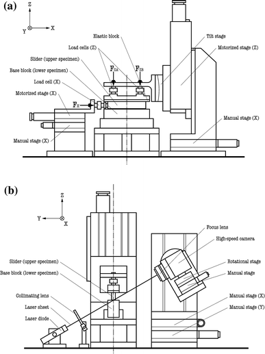
Schematic diagram of the experimental apparatus with a transmissive optical system: a front view and b side view
- F ZB :
-
Partial normal load (N) (Fig. 1a)
- k :
-
Stiffness of the material section (N/m) (Eq. 10)
- K :
-
Stiffness of the loading section (N/m)
- L :
-
Length of the slider (m)
- L p :
-
Propagation length of precursors (m)
- m :
-
Mass (kg) (Eq. 9)
- M :
-
Mass of the slider (kg)
- N :
-
Number of blocks
- S :
-
Cross-section area of the slider (m2)
- t :
-
Time (s)
- V :
-
Driving speed (m/s)
- w i :
-
Normal load (N) (Eq. 7)
- x i :
-
Position (m)
- y i :
-
Spring compression (m) (Eq. 11)
- \( y_{i}^{\max } \) :
-
Maximum spring compression (m)
- θ:
-
Degree of non-uniformity of normal loading
- μk :
-
Kinetic friction coefficient
- μs :
-
Static friction coefficient
- μsapp :
-
Apparent static friction coefficient (Eq. 1)
- (•):
-
Derivative with respect to time t

References
Den Hartog, J.P.: Mechanical Vibration, 4th edn. McGraw-Hill, New York (1956)
Pratt, T.K., Williams, R.: Non-linear analysis of stick/slip motion. J. Sound Vib. 74, 531–542 (1981)
Paliwal, M., Mahajan, A., Don, J., Chu, T., Filip, P.: Noise and vibration analysis of a disc-brake system using a stick-slip friction model involving coupling stiffness. J. Sound Vib. 282, 1273–1284 (2005)
Scholz, C.H.: The Mechanics of Earthquakes and Faulting, 2nd edn. Cambridge University Press, Cambridge (2002)
Ohnaka, M., Kuwahara, Y.: Characteristic features of local breakdown near a crack-tip in the transition zone from nucleation to unstable rupture during stick-slip shear failure. Tectonophys 175, 197–220 (1990)
Nakanishi, H.: Statistical properties of the cellular-automaton model for earthquakes. Phys. Rev. A 43, 6613–6621 (1991)
Braun, O.M., Roder, J.: Transition from stick-slip to smooth sliding: an earthquakelike model. Phys. Rev. Lett. 88, 096102 (2002)
Bykov, V.G.: Stick-slip and strain waves in the physics of earthquake rupture: experiments and models. Acta Geophys. 56, 270–285 (2008)
Dieterich, J.H., Kilgore, B.D.: Direct observation of frictional contacts: new insights for state-dependent properties. Pure Appl. Geophys. 143, 283–302 (1994)
Bowden, F.P., Tabor, D.: The Friction and Lubrication of Solids. Oxford University Press, Oxford (1950)
Persson, B.N.J.: Sliding Friction, 2nd edn. Springer, New York (2000)
Nakano, K.: Two dimensionless parameters controlling the occurrence of stick-slip motion in a 1-DOF system with Coulomb friction. Tribol. Lett. 24, 91–98 (2006)
Nakano, K., Maegawa, S.: Safety-design criteria of sliding systems for preventing friction-induced vibration. J. Sound Vib. 324, 539–555 (2009)
Nakano, K., Maegawa, S.: Stick-slip in sliding systems with tangential contact compliance. Tribol. Int. 42, 1771–1780 (2009)
Nakano, K., Maegawa, S.: Occurrence limit of stick-slip: dimensionless analysis for fundamental design of robust stable systems. Lubr. Sci. 22, 1–18 (2010)
Gerde, E., Marder, M.: Friction and fracture. Nature 413, 285–288 (2001)
Baumberger, T., Caroli, C., Ronsin, O.: Self-healing slip pulses along a gel/glass interface. Phys. Rev. Lett. 88, 075509 (2002)
Xia, K., Rosakis, A.J., Kanamori, H.: Laboratory earthquakes: the sub-Rayleigh-to-supershear rupture transition. Science 303, 1859–1861 (2004)
Rubinstein, S.M., Cohen, G., Fineberg, J.: Detachment fronts and the onset of dynamic friction. Nature 430, 1005–1009 (2004)
Rubinstein, S.M., Shay, M., Cohen, G., Fineberg, J.: Crack-like processes governing the onset of frictional slip. Int. J. Fract. 140, 201–212 (2006)
Rubinstein, S.M., Cohen, G., Fineberg, J.: Dynamics of precursors to frictional sliding. Phys. Rev. Lett. 98, 226103 (2007)
Braun, O.M., Barel, I., Urbakh, M.: Dynamics of transition from static to kinetic friction. Phys. Rev. Lett. 103, 194301 (2009)
Bureau, L., Baumberger, T., Caroli, C.: Rheological aging and rejuvenation in solid friction contacts. Eur. Phys. J. E 8, 331–337 (2002)
Richeton, J., Ahzi, S., Vecchio, K.S., Jiang, F.C., Adharapurapu, R.R.: Influence of temperature and strain rate on the mechanical behavior of three amorphous polymers: characterization and modeling of the compressive yield stress. Int. J. Solids Struct. 43, 2318–2335 (2006)
Carlson, J.M., Langer, J.S.: Mechanical model of an earthquake fault. Phys. Rev. A 40, 6470–6484 (1989)
Author information
Authors and Affiliations
Corresponding author
Rights and permissions
About this article
Cite this article
Maegawa, S., Suzuki, A. & Nakano, K. Precursors of Global Slip in a Longitudinal Line Contact Under Non-Uniform Normal Loading. Tribol Lett 38, 313–323 (2010). https://doi.org/10.1007/s11249-010-9611-7
Received:
Accepted:
Published:
Issue Date:
DOI: https://doi.org/10.1007/s11249-010-9611-7