
Abstract
In this paper, we construct a new car-following model with inter-vehicle communication (IVC) to study the driving behavior under an accident. The numerical results show that the proposed model can qualitatively describe the effects of IVC on each vehicle’s speed, acceleration, movement trail, and headway under an accident and that the new model can overcome the full velocity difference (FVD) model’s shortcoming that collisions occur under an accident, which illustrates that the new model can better describe the driving behavior under an accident than the FVD model.
1 Introduction
To date, traffic problems have been serious and attracted researchers to develop traffic flow models to explore the complex traffic phenomena (e.g., lane-changing, congestion, local clusters, phase transition, etc.) [1, 2]. Roughly speaking, these models can be divided into micro models [3–19] and macro models [20–41], where the micro models focus on studying the micro properties of traffic flow (e.g., lane-changing, overtaking, etc.) and the macro models focus on exploring the macro properties of traffic flow (e.g., the fundamental diagram, the distribution, evolution, propagation of density, speed and flow, etc.). However, the above models cannot be used to explore the effects of inter-vehicle communication (IVC) on traffic flow since IVC is not explicitly considered in these models.
With the development of the computer technology, IVC has been an important tool that driver can receive the related information from his/her traffic state, so IVC can help driver to better adjust his/her driving behavior. To explore the impacts of IVC on traffic flow, researchers developed some models to study the properties of traffic flow in the traffic system with IVC. Tsugawa [42] gave an overview on IVC and its application, defined IVC as a communication among the vehicles under intelligent-transportation system (ITS), and pointed out that IVC can effectively enlarge the horizon of the drivers and on-board sensors. Knorr et al. [43] explored the mixed traffic flow consisting of the vehicles with and without IVC, thus they constructed an effective strategy that can improve the stability of traffic flow. Jin and Recker [44] discussed the reliability of IVC under one traffic stream and found that the reliability is dependent on the distribution of the vehicles with IVC but directly related to the proportion of the vehicles with IVC. Kerner et al. [45] developed a test-bed for the wireless IVC based on their three-phase traffic theory and studied the statistical features of ad hoc vehicle networks and the influences of car-to-car (C2C) communication on the traffic efficiency and safety. Ngoduy et al. [46] applied the multi-class gas-kinetic theory to obtain the speed of the vehicles with IVC based on the downstream traffic state, thus they proposed a continuum model to investigate the dynamics properties of cooperative traffic flow. However, the above models [42–46] do not study the effects of IVC on the micro driving behavior since they did the research from the macroscopic perspective. In fact, IVC will affect the micro driving behavior. For example, IVC can provide drivers information (e.g., road quality) which can help drivers to adjust their driving behavior, so IVC should explicitly be considered when we explore the micro driving behavior. However, IVC often has significant impacts on the micro driving behavior only when large perturbation (e.g., accident) occurs in the traffic system. Therefore, we in this paper construct a car-following model with IVC to study the effects of IVC on the driving behavior under an accident.
2 Model
The existing car-following models on a single lane can be written as follows [3–11]:
where \(v_\mathrm{n} ,\Delta x_\mathrm{n} = x_{\mathrm{n}+1} -x_\mathrm{n} ,\Delta v_\mathrm{n} =v_{\mathrm{n}+1} -v_\mathrm{n} ,x_\mathrm{n} \) are respectively the nth vehicle’s speed, headway, relative speed, and position. Equation (1) illustrates that the nth vehicle’s acceleration is determined by its speed, headway, relative speed, and other factors (e.g., multi-anticipative speed and speed difference, road quality, etc.).Footnote 1 If we define Eq. (1) as different formulations, we can obtain different car-following models. For instance, Lenz et al. [17] extended the car-following model [3–5] by incorporating multi-vehicle interactions and proved that multi-vehicle interactions can improve the stability of traffic flow; Hoogendoorn et al. [18] applied empirical trajectory data to analyze the heterogeneous multi-anticipative behavior and found that considering the multi-anticipative behavior can greatly improve the performance of their proposed car-following model; Treiber et al. [19] generalized many time-continuous car-following models and found that the essential aspects of driver behavior (e.g., the finite reaction time, estimation errors, spatial anticipation, and temporal anticipation) cannot be captured by the models.
However, IVC is not explicitly considered in the above car-following models, so these car-following models cannot be used to study the effects of IVC on the driving behavior. In fact, IVC can provide drivers information, so it will affect the driving behavior and should be explicitly considered if we apply car-following model to study the driving behavior in the traffic system with IVC. Among the existing car-following models, the full velocity difference model (FVD) [7] has widely been extended to investigate the driving behavior because it has been cited 175 times since 2001 based on the data from the web of science, so we can here propose a car-following model to study the influences of IVC on the driving behavior based on the FVD model [7]. But IVC often affects the parameters \({\kappa },{\lambda }\) and the optimal velocity \(V\left( {\Delta x_\mathrm{n}}\right) \) in the FVD model and produces a perturbed term on the basis of the FVD model, so we can construct a car-following model with consideration of IVC based on the FVD model [7], i.e.,
where \(V_{\mathrm{IVC}}\left( {\Delta x_\mathrm{n}\left( t\right) } \right) \) is the nth vehicle’s optimal speed with consideration of IVC, \(\kappa _{\mathrm{IVC}},\lambda _{\mathrm{IVC}}\) are two reaction coefficients whose physical meanings are similar to those of \({\kappa },{\lambda }\) in the FVD model [7], \(\xi _{\mathrm{IVC}}\) is the perturbed term resulted by IVC.
\(V_{\mathrm{IVC}}\left( {\Delta x_\mathrm{n}\left( t\right) } \right) \) is related to the vehicle’s performance and ICV cannot change each vehicle’s performance, so we can define it as follows [3]:
where \(v_{\mathrm{max}}\) is the maximum speed, \(x_\mathrm{c}\) is the safety distance. As for the parameters \(\kappa _{\mathrm{IVC}},\lambda _{\mathrm{IVC}}\), we will define them in the next section.
Roughly seeing, the proposed model is similar to the model [11], but they have the following difference: the drivers can adjust their acceleration in Eq. (2) based on all the traffic situations in front of them since they can obtain the traffic information through IVC while the drivers can adjust their acceleration in model [11] only based on the traffic situations within their sight. For example, when an accident occurs, the drivers can immediately adjust their acceleration based on Eq. (2) since they can know the accident and its related information through IVC, while the drivers still drive their vehicles based on the traffic situations within their sight in the model [11] because they cannot immediately know the accident. The above difference shows that the model [11] cannot describe the effects of IVC on the driving behavior and that Eq. (2) can be used to study the driving behavior in the traffic system with IVC.
3 Numerical tests
Equation (2) consists of multi ODEs that are non-autonomous systems and many parameters of the proposed are discontinuous, so it is very difficult to obtain its analytical solution and carry out its stability analysis, but we will further explore this topic in the future. Therefore, we should here use numerical scheme to discretize Eq. (2). However, there are many different numerical schemes that can be used to discretize Eq. (2), but the schemes have no qualitative effects on the numerical results, so we here apply the Euler forward difference to discretize Eq. (2), i.e.,
where \(\Delta t=1\mathrm {s}\) is the length of the time-step.
Before simulation, we should first define \(\xi _{\mathrm{IVC}}, \kappa _{\mathrm{IVC}}\), \(\lambda _{\mathrm{IVC}}, v_{\mathrm{IVC}}^{\max }, x_{\mathrm{IVC}}^\mathrm{c}\). In the following numerical tests, we use Eq. (2) to explore the evolution of traffic flow when an accident occurs in a traffic system. Once the accident occurs, IVC will provide the drivers some related information, so the drivers at the accident’s upstream will decelerate more quickly, i.e., \(\xi _{\mathrm{IVC}} <0, \kappa _{\mathrm{IVC}} ,\lambda _{\mathrm{IVC}} \) are larger than those of FVD model. Similarly, IVC will provide related information once the accident is cleared, so \(\xi _{\mathrm{IVC}} >0, \kappa _{\mathrm{IVC}},\lambda _{\mathrm{IVC}} \) are larger than those of FVD model. But \(\xi _{\mathrm{IVC}},\kappa _{\mathrm{IVC}},\lambda _{\mathrm{IVC}} \) have no qualitative impacts on the numerical results, so we here simplify them as follows:
where \(t_{0}\) is the time that the accident occurs, \(T_{\mathrm{accident}}\) is the time that the accident is cleared, \(-\xi _\mathrm{i},\beta _\mathrm{i} ,\lambda _\mathrm{i}\) are the corresponding perturbed terms resulted by IVC under the accident, \(\kappa ,\lambda \) are the corresponding parameters without IVC. For simplicity, we here define \(t_{0}=0\).
During the period from the time that the accident occurs to the time that the accident is cleared, the effects of IVC and accident will turn weaker with the increase of the distance between the vehicle and accident, which shows that \(\xi _{1},\beta _{1},\lambda _{1}\) will decrease with the increase of the distance between the vehicle and accident, so we can here define \(\xi _{1},\beta _{1},\lambda _{1} \) as follows:
where \(\xi _{1,\mathrm{max}},\beta _{1,\mathrm{max}},\lambda _{1,\mathrm{max}}\) are the corresponding maximum values, x is the vehicle’s position, \(x_{0}\) is the accident’s position, D is a critical value.
Similarly, after the accident is cleared, the effects of IVC under the accident are related to the distance between the first vehicle and the current vehicle, i.e., the impacts will increase with the distance, so \(\xi _{2},\beta _2,\lambda _{2} \) will increase with the distance, so we can for simplicity define \(\xi _{2},\beta _2,\lambda _{2} \) as follows:
In this paper, we study the effects of IVC on the driving behavior. The initial conditions of the numerical tests are as follows:
where N is the number of vehicles.
Other parameters are defined as follows:
Researchers often carry out the linear stability analysis and nonlinear analysis of car-following model, but as for the stability of Eq. (2), we here give the following note: IVC affects the driving behavior only when one accident occurs. But since accident belongs to a large perturbation, we do not use linear stability analysis or nonlinear analysis to study the impacts of IVC on each vehicle’s driving behavior since the two methods can only be used to explore small perturbation.
However, we can study the effects of IVC on each vehicle’s driving behavior during the period from the time when an accident occurs to the time when the queue is dissipated from the analytical perspective. Using the above definitions of the related parameters, we can obtain the following proposition.
Proposition
When the accident occurs and before it is cleared, each vehicle’s deceleration of the proposed model is greater than the one of the FVD model under the same condition, i.e.,\(a_\mathrm{n}\ge \bar{{a}}_\mathrm{n} \ge 0\); after the accident is cleared and before the queue is dissipated, each vehicle’s acceleration obtained by the proposed model is greater than the one of the FVD model under the same conditions, i.e., \(a_\mathrm{n}\ge \bar{{a}}_\mathrm{n}\ge 0\). Footnote 2
Proof
When the accident occurs and before it is cleared, we have
Using the above definitions of the related parameters, we have
Thus, under the same condition, we have
After the accident is cleared and before the queue is dissipated, we have
Using the above definitions of the related parameters, we have
Thus, under the same condition, we have
The above proposition shows that IVC have positive effects on each vehicle’s motion during the period from the time that the accident occurs to the time that the queue is dissipated, i.e.,
-
(i)
When the accident occurs and before it is cleared, IVC can lessen the braking process of the vehicles which should stop, which can improve the traffic safety.
-
(ii)
After the accident is cleared and before the queue is dissipated, ICV can lessen the starting process of the vehicles, which can speed up the dissipation speed of the queue.
To validate the above proposition, we apply the above conditions to carry out some numerical tests, where each vehicle’s speed, acceleration, running trail, and headway under an accident are shown in Figs. 1, 2, 3, and 4. From these figures, we can obtain the following results:
-
(1)
Because IVC can guide each driver to decelerate in advance before the accident is cleared, each vehicle’s speed obtained by the new model is less than the one obtained by the FVD model. Since IVC can enhance each driver’s acceleration and speed when the accident is cleared, each vehicle’s speed of the FVD model is less than that of the new model, each vehicle can quickly start, its speed quickly increase to its ideal speed, and each vehicle’s starting time of the new model is shorter than that of the FVD model (Fig. 1).
-
(2)
Each vehicle decelerates but its deceleration of the new model is greater than that of the FVD model before the accident is cleared, so each vehicle’s braking time of the new model is shorter than that of the FVD model. Each vehicle accelerates but its acceleration of the FVD model is less than that of the new model after the accident is cleared, so each vehicle’s starting time of the new model is shorter than that of the FVD model (Fig. 2).
-
(3)
Before the accident is cleared, some collisions will occur under the FVD model and no collision occurs under the new model, so the new model can avoid collision and is better than the FVD model (Fig. 3).
-
(4)
Because the FVD model will produce collision under an accident, we only draw each vehicle’s headway of the proposed model. Before the accident is cleared, each vehicle’s headway is relatively large in order to avoid collision; once the accident is cleared, each vehicle’s headway is relatively small in order that the vehicles’ queue can quickly be dissipated; the vehicles’ headways far away from the accident are approximately equal to the initial headway since the accident and IVC have little effects on the vehicles’ driving behavior (Fig. 4).
Fig. 1 
Each vehicle’s speed under \(N=20,T_{\mathrm{{accident}}} =300\) s, where a and b are, respectively, the results of the FVD model and c and d are the results of the proposed model
Fig. 2 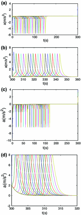
Each vehicle’s acceleration under \(N=20,T_{\mathrm{{accident}}}=300\) s, where a and b are, respectively, the results of the FVD model and c and d are the results of the proposed model
Fig. 3 
Each vehicle’s running trail under \(N=20,T_{\mathrm{{accident}}}=300\) s, where a and b are, respectively, the results of the FVD model and the proposed model
Fig. 4 
Each vehicle’s headway under the proposed model, where \(N=20,T_{\mathrm{{accident}}}=300\) s


4 Conclusions
In this paper, we propose a car-following model to study the impacts of IVC on each vehicle’s speed, acceleration, running trail, and headway under an accident. The numerical results show that the new model can qualitatively describe each vehicle’s velocity, acceleration, running trail, and headway.
However, this paper has the following limitations:
-
(1)
The proposed model is not deduced from the experimental data;
-
(2)
All the parameters are not calibrated by used of experimental data
-
(3)
We do not study the impacts of IVC on the driving behavior under other traffic states.
In view of the above limitations, in the future we will use experimental data to construct an exact car-following model to further study the effects of IVC on the driving behavior under other traffic states.
References
Chowdhury, D., Santen, L., Schreckenberg, A.: Statistics physics of vehicular traffic and some related systems. Phys. Rep. 329, 199–329 (2000)
Helbing, D.: Traffic and related self-driven many-particle systems. Rev. Mod. Phys. 73, 1067–1141 (2001)
Bando, M., Hasebe, K., Nakayama, A., Shibata, A., Sugiyama, Y.: Dynamical model of traffic congestion and numerical simulation. Phys. Rev. E 51, 1035–1042 (1995)
Bando, M., Hasebe, K., Nakanishi, K.: Phenomenological study of dynamical model of traffic flow. J. Phys. I 5, 1389–1399 (1995)
Herrmann, M., Kerner, S.: Local cluster effect in different traffic flow models. Physica A 255, 163–188 (1998)
Nagatani, T.: Stabilization and enhancement of traffic flow by next-nearest-neighbor interaction. Phys. Rev. E 60, 6395–6401 (1998)
Jiang, R., Wu, Q.S., Zhu, Z.J.: Full velocity difference model for car-following theory. Phys. Rev. E 64, 017101 (2001)
Zhao, X.M., Gao, Z.Y.: A new car-following model: full velocity and acceleration difference model. Eur. Phys. J. B 47, 145–150 (2005)
Li, Y., Sun, D., Liu, W., Zhang, M., Zhao, M., Liao, X., Tang, L.: Modeling and simulation for microscopic traffic flow based on multiple headway, velocity and acceleration difference. Nonlinear Dyn. 66, 15–28 (2011)
Tang, T.Q., Wu, Y.H., Caccetta, L., Huang, H.J.: A new car-following model with consideration of roadside memorial. Phys. Lett. A 375, 3845–3850 (2011)
Tang, T.Q., Wang, Y.P., Yang, X.B., Wu, Y.H.: A new car-following model accounting for varying road condition. Nonlinear Dyn. 70, 1397–1405 (2012)
Naito, Y., Nagatani, T.: Effect of headway and velocity on safety-collision transition induced by lane changing in traffic flow. Physica A 391, 1626–1635 (2012)
Nagatani, T., Tobita, K.: Vehicular motion in counter traffic flow through a series of signals controlled by a phase shift. Physica A 391, 4976–4985 (2012)
Tobita, K., Nagatani, T.: Effect of signals on two-route traffic system with real-time information. Physica A 391, 6137–6145 (2012)
Nagatani, T.: Nonlinear-map model for bus schedule in capacity-controlled transportation. Appl. Math. Model. 37, 1823–1835 (2013)
Sugiyama, N., Nagatani, T.: Multiple-vehicle collision in traffic flow by a sudden slowdown. Physica A 392, 1848–1857 (2013)
Lenz, H., Wagner, C.K., Sollacher, R.: Multi-anticipative car-following model. Eur. Phys. J. B 7, 331–335 (1999)
Hoogendoorn, S.P., Ossen, S., Schreuder, M.: Properties of a microscopic heterogeneous multi-anticipative traffic flow model. In: Allsop, R.E., Bell, M.G.H., Heydecker Benjamin, G. (eds.) Transportation and Traffic Theory. Elsevier, Oxford (2007)
Treiber, M., Kesting, A., Helbing, D.: Delays, inaccuracies and anticipation in microscopic traffic models. Physica A 360, 71–88 (2006)
Lighthill, M.J., Whitham, G.B.: On kinematic waves: II. A theory of traffic flow on long crowed roads. Proc. R. Soc. Lond. 229, 317–345 (1955)
Richards, P.I.: Shock waves on the highway. Oper. Res. 4, 42–51 (1956)
Payne, H.J.: Models of freeway traffic and control. In: Bekey, G.A. (ed.) Mathematical Models of Public System. Simulation Councils Proceedings Series, vol. 1, pp. 51–61 (1971)
Jiang, R., Wu, Q.S., Zhu, Z.J.: A new continuum model for traffic flow and numerical tests. Transp. Res. B 36, 405–419 (2002)
Bellomo, N., Delitala, M., Coscia, V.: On the mathematical theory of vehicular traffic flow I: fluid dynamic and kinematic modeling. Math. Models Methods Appl. Sci. 12, 1801–1843 (2002)
Gupta, A.K., Katiyar, V.K.: Analyses of shock waves and jams in traffic flow. J. Phys. A 38, 4063–4069 (2005)
Gupta, A.K., Katiyar, V.K.: A new anisotropic continuum model for traffic flow. Physica A 368, 551–559 (2006)
Gupta, A.K., Katiyar, V.K.: Phase transition of traffic states with on-ramp. Physica A 371, 674–682 (2006)
Gupta, A.K., Katiyar, V.K.: A new multi-class continuum model for traffic flow. Transportmetrica 3, 73–85 (2007)
Delitala, M., Tosin, A.: Mathematical modelling of vehicular traffic: a discrete kinetic theory approach. Math. Models Methods Appl. Sci. 17, 901–932 (2007)
Bellouquid, A., Delitala, M.: Asymptotic limits of a discrete kinematic theory model of vehicular traffic. Appl. Math. Lett. 24, 672–678 (2011)
Tang, T.Q., Caccetta, L., Wu, Y.H., Huang, H.J., Yang, X.B.: A macro model for traffic flow on road networks with varying road conditions. J. Adv. Transp. (2011). doi:10.1002/atr.215
Ngoduy, D.: Multiclass first order modelling of traffic networks using discontinuous flow-density relationships. Transportmetrica 6, 121–141 (2010)
Gupta, A.K., Sharma, S.: Nonlinear analysis of traffic jams in an anisotropic continuum model. Chin. Phys. B 19, 110503 (2010)
Gupta, A.K., Sharma, S.: Analysis of the wave properties of a new two-lane continuum model with the coupling effect. Chin. Phys. B 21, 015201 (2012)
Ngoduy, D.: Multiclass first-order traffic model using stochastic fundamental diagrams. Transportmetrica 7, 111–125 (2011)
Peng, G.H., Nie, Y.F., Cao, B.F., Liu, C.Q.: A driver’s memory lattice model of traffic flow and its numerical simulation. Nonlinear Dyn. 67, 1811–1815 (2012)
Ngoduy, D.: Effect of driver behaviours on the formation and dissipation of traffic flow instabilities. Nonlinear Dyn. 69, 969–975 (2012)
Ngoduy, D., Maher, M.J.: Calibration of second order traffic models using continuous cross entropy method. Transp. Res. C 24, 102–121 (2012)
Ngoduy, D.: Instability of cooperative adaptive cruise control traffic flow: a macroscopic approach. Commun. Nonlinear Sci. Numer. Simul. 18, 2838–2851 (2013)
Ngoduy, D.: Analytical studies on the instabilities of heterogeneous intelligent traffic flow. Commun. Nonlinear Sci. Numer. Simul. 18, 2699–2706 (2013)
Peng, G.H.: A new lattice model of the traffic flow with the consideration of the driver anticipation effect in a two-lane system. Nonlinear Dyn. 73, 1035–1043 (2013)
Tsugawa, S.: Inter-vehicle communications and their applications to intelligent vehicles: an overview. Intell. Veh. Symp. IEEE 2, 564–569 (2002)
Knorr, F., Schreckenberg, M.: Influence of inter-vehicle communication on peak hour traffic flow. Physica A 6, 2225–2231 (2012)
Jin, W.L., Recker, W.W.: Instantaneous information propagation in a traffic stream through inter-vehicle communication. Transp. Res. B 3, 230–250 (2006)
Kerner, B.S, Klenov, S.L, Brakemeier, A.: Testbed for wireless vehicle communication: a simulation approach based on three-phase traffic theory. In: Intelligent Vehicles Symposium IEEE, pp. 180–185 (2008)
Ngoduy, D., Hoogendoorn, S.P., Liu, R.: Continuum modeling of cooperative traffic flow dynamics. Physica A 13, 2705–2716 (2009)
Acknowledgments
This study has been supported by the National Natural Science Foundation of China (71271016) and the National Basic Research Program of China (2012CB725404). The authors would like to thank the anonymous referees for their helpful comments and valuable suggestions which have improved the paper substantially.
Author information
Authors and Affiliations
Corresponding author
Rights and permissions
About this article
Cite this article
Tang, T., Shi, W., Shang, H. et al. A new car-following model with consideration of inter-vehicle communication. Nonlinear Dyn 76, 2017–2023 (2014). https://doi.org/10.1007/s11071-014-1265-9
Received:
Accepted:
Published:
Issue Date:
DOI: https://doi.org/10.1007/s11071-014-1265-9