Darboux transformation for an integrable generalization of the nonlinear Schrödinger equation

Abstract

A Darboux transformation for an integrable generalization of the coupled nonlinear Schrödinger equation is derived with the help of the gauge transformation between the Lax pair. As a reduction, a Darboux transformation for an integrable generalization of the nonlinear Schrödinger equation is obtained, from which some new solutions for the integrable generalization of the nonlinear Schrödinger equation are given.

1 Introduction

In [1], Fokas proposed an integrable generalization of the nonlinear Schrödinger (NLS) equation

(1)

by using bi-Hamiltonian methods, where γ and ν are nonzero real parameters and u(x,t) is a complex-valued function. Equation (1) reduces to the NLS equation when ν=0, and it arises as a model for nonlinear pulse propagation in monomode optical fibers and is the first negative member of the integrable hierarchy associated with the derivative NLS equation [2]. In [3], Lenells and Fokas used the bi-Hamiltonian structure to write down the first few conservation laws of (1) and derive its Lax pair, by which they solve the initial value problem and analyze solitons. The initial-boundary value problem for (1) on the half-line was studied in [4]. In particular, the so-called linearizable boundary conditions were considered. Furthermore, a particular solution was used to verify explicitly all the steps needed for the solution of a well-posed problem. Recently, Lenells implemented the dressing method for (1) and derived explicit formulas for the N-soliton solutions [5].

The aim of the present paper is to study the integrable generalization of the NLS equation with the aid of the Darboux transformation (DT). It is known that the DT is a powerful tool which generates new solutions of an integrable equation from an already known seed solution [6–10]. The DT approach possesses a lot of advantages compared with other methods. For example, if the obtained solutions are taken as the new starting point, one can make the DT once again and engender another set of new solutions. This process can be done continually and will usually yield a series of new explicit solutions. Here, we first construct a DT for an integrable generalization of the coupled NLS equation with the aid of a gauge transformation between the corresponding matrix spectral problems. As a reduction, a DT for the integrable generalization of the NLS equation is obtained. A systematic algebraic procedure is given in detail to solve the integrable generalization of the NLS equation, from which some new explicit solutions are derived.

The present paper is organized as follows. In Sect. 2, we shall construct a DT for the integrable generalization of the coupled NLS equation resorting to the gauge transformation between matrix spectral problems. In Sect. 3, a DT for the integrable generalization of the NLS equation is discussed through the reduction technique. Furthermore, two classes of new explicit solutions for the integrable generalization of the NLS equation are derived by the application of its DT.

2 Darboux transformation

In this section, we shall construct a DT for an integrable generalization of the coupled NLS equation

$$\begin{array}{rcl}u_{xt}+\alpha\beta^2u-2i\alpha \beta u_x-\alpha u_{xx}+i\alpha\beta^2uvu_x=0,\cr\noalign{\vspace{3pt}}v_{xt}+\alpha\beta^2v+2i\alpha\beta v_x-\alpha v_{xx}-i\alpha\beta^2uvv_x=0,\end{array} $$

(2)

which comes from the condition of the compatibility for two matrix spectral problems [3]:

(3)

(4)

where u and v are two potentials with independent variables x and t, ζ is a constant spectral parameter, and

$$\eta=\sqrt{\alpha}\biggl(\zeta-\frac{\beta}{2\zeta}\biggr). $$

(5)

Under a certain transformation (see Sect. 3 below), (2) is reduced the integrable generalization of the NLS equation (1), which has important applications in physics.

In what follows, we shall derive a DT for the integrable generalization of the coupled NLS equation (2). Let ϕ=(ϕ ₁,ϕ ₂)^T,ψ=(ψ ₁,ψ ₂)^T be two basic solution of (3). We use (ϕ,ψ) to define the linear algebraic system

(6)

with

(7)

where parameters ζ _j and γ _j (ζ _k ≠ζ _j ,γ _k ≠γ _j ,k≠j) are suitably chosen such that the determinants of the coefficients for (6) are nonzero. Hence, A _k ,B _k ,C _k , and D _k (k=1,…,N) are uniquely determined by (6). Now we introduce a gauge transformation of the spectral problem (3)

(8)

where

From (6), we have

that is

(9)

Equation (9) implies that $\zeta_{j}^{2}\ (j=1,\ldots,2N)$ are 2N roots of the (4N)th-order polynomial detT. Therefore, we have

(10)

Under the gauge transformation (8), the spectral problem (3) is transformed into the following spectral problem of $\tilde{\psi}$ when ζ≠ζ _j (j=1,…,2N):

(11)

where

(12)

It turns out that ζ=ζ _j (j=1,…,2N) are removable isolated singularities of $\tilde{M}$ (see (13) below). Thus, we can define $\tilde{M}$ for all ζ by analytic continuation.

Theorem 1

The matrix $\tilde{M}$ determined by (12) has the same form as M:

(13)

where the transformation formulae from the old potentials u and v into new ones are given by

(14)

The transformation determined by (8) and (14): $(\psi;u,v)\rightarrow(\tilde{\psi};\tilde{u},\tilde{v})$ is usually called a DT of the spectral problem (4).

Proof

Let T ⁻¹=T ^∗/detT and

(15)

A direct calculation shows that f ₁₁(ζ), f ₂₂(ζ),ζf ₁₂(ζ), ζf ₂₁(ζ) are (2N+1)th-order polynomials in ζ². By using (3), (6), and (7), we have

(16)

(17)

Resorting to (16) and (17), it can be verified that ζ _j (j=1,…,2N) are roots of f _kl (k,l=1,2) in (15). Therefore, we have from (10) that

(18)

with

where $p_{kl}^{(j)}$ are independent of ζ. Equation (18) can be written as

(19)

Equating the coefficients of ζ^2N+2,ζ, and ζ⁰ in (19), we obtain

(20)

(21)

Substituting (14) and (20) into (21) yields

(22)

The proof is thus completed. □

Remark 1

Equating the coefficients of ζ^2N+1 in (19), we have

(23)

By virtue of (20) and (22), we obtain

(24)

Assume that the two solutions ϕ and ψ of (3) satisfy (4) as well. Differentiating $\tilde{\psi}=T\psi$ with respect to t yields

(25)

Then we can prove the following assertion.

Theorem 2

The matrix $\tilde{N}$ defined by the second expression of (25) has the same form as N, in which the old potentials u and v are mapped into $\tilde{u}$ and $\tilde{v}$ according to the same DT (14).

Proof

Let T ⁻¹=T ^∗/detT and

(26)

A direct calculation shows that ζ² g ₁₁(ζ) and ζ² g ₂₂(ζ) are (2N+2)th-order polynomials in ζ², ζg ₁₂(ζ), and ζg ₂₁(ζ) are (2N+1)th-order polynomials in ζ². By virtue of (4), (7), and (17), we have

(27)

where $\eta_{j}=\sqrt{\alpha}(\zeta_{j}-\frac{\beta}{2\zeta_{j}})$. It can be easily verified by (16), (17), and (27) that ζ _j (j=1,…,2N) are roots of g _kl (ζ),k,j=1,2. Therefore, we arrive at

(28)

with

where $q_{kl}^{(j)}$ are independent of ζ. Equation (28) can be written as

(29)

By comparing the coefficients of ζ^2N+2,ζ⁻²,ζ⁻¹, and ζ⁰ in (29), we get

(30)

(31)

By using (14), we obtain

(32)

Equating the coefficients of ζ^2N+1 in (29), we have

which together with (24) implies

(33)

The proof is thus completed. □

According to Theorems 1 and 2, the transformation (8) and (14) converts the Lax pair (3) and (4) into another Lax pair of the same type (11) and (25). Therefore, both of the Lax pairs lead to the same integrable generalization of the coupled NLS equation (2). The transformation (14) is also called a DT for the integrable generalization of the coupled NLS equation (2). We get immediately the following fact.

Theorem 3

Every solution (u,v) for the integrable generalization of the coupled NLS equation (2) is mapped into a new solution $(\tilde{u},\tilde{v})$ for the integrable generalization of the coupled NLS equation (2) under the DT (14), where B ₁ and C ₁ are given by the linear algebraic system (6).

3 The reduction of Darboux transformation and application

In this section, we will use the reduction technique to derive a DT for the integrable generalization of the NLS equation. Let $\alpha=\frac{\gamma}{\nu}>0$ and $\beta=\frac{1}{\nu}$. Then the transformation, $u \rightarrow\beta\sqrt{\alpha}\ e^{i\beta x}u$, σ→−σ, converts (1) into [5]

(34)

which is equivalent to (1) because the above transformation is invertible. Without loss of generality, in the rest of the paper we will concentrate on the integrable generalization of the NLS equation (34). It is easy to see that (2) reduces to (34) as well when v=σu ^∗. Therefore, we always assume that v=σu ^∗ as follows. In this case, we choose two solutions of (3) and (4):

(35)

and parameters

(36)

By using (6) and (7), we obtain $\alpha_{2j}^{-1}=\sigma\alpha^{*}_{2j-1},\ D_{k}= A^{*}_{k}, \ C_{k}=\sigma B^{*}_{k}, \ (j=1,\ldots,N; k=1,\ldots,N)$. Here, α _2j−1 is given by

(37)

functions A _k and B _k are determined by the following linear algebraic system

(38)

According to (14) and v=σu ^∗, we arrive at $\tilde{v}=v+C_{1}=\sigma u^{*}+\sigma B_{1}^{*}=\sigma\tilde{u}^{*}$, which implies that $\tilde{v}=\sigma\tilde{u}^{*}$. Therefore, we prove easily the following assertion.

Theorem 4

Every solution u for the integrable generalization of the NLS equation (34) is mapped into a new solution $\tilde{u}$ under the DT

(39)

where B ₁ is determined by (38).

In the following, we shall apply the DT to give explicit solutions for the integrable generalization of the NLS equation (34). Substituting the trivial solution u=0 (v=σu ^∗=0) of (34) into (3) and (4), their two basic solutions ϕ(ζ) and ψ(ζ) are chosen as

(40)

in the view of (35). Then (37) and (38) can be written as

(41)

(42)

Using the DT, we obtain exact solutions for the integrable generalization of the NLS equation (34):

(43)

where B ₁ is determined by (42). For simplicity, we shall discuss the two special cases N=1 and N=2.

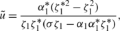
• (I) For N=1, a direct calculation gives from (42) that

  

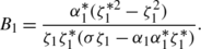
  According to the Darboux transformation (39), we get a one-soliton solution for the integrable generalization of the NLS equation (34)

  

  (44)

  with $\alpha_{1}=-\gamma_{1}\exp(2i\zeta_{1}^{2}x+2i\eta_{1}^{2}t), \ \eta_{1}= \sqrt{\alpha}(\zeta_{1}-\frac{\beta}{2\zeta_{1}})$. Plots of this solution are given in Fig. 1 if the parameters are chosen as α=1,β=−1,σ=−1,ζ₁=0.6+0.2i,γ ₁=0.5+0.8i (see Fig. 1).

  Fig. 1

  

  One-soliton solution

• (II) For N=2, we obtain from linear algebraic system (42) that

  

  (45)

  which is a two-soliton solution of (34), where

  
  
  

  Plots of this solution are given in Fig. 2 if the parameters are chosen as α=1,β=−1,σ=−1,ζ₁=0.48+0.3i,γ ₁=0.05+0.15i,ζ₃=0.064+0.37i,γ ₃=0.98+0.99i (see Fig. 2).

  Fig. 2

  

  Two-soliton solution

  Now we choose two seek solutions of (34) as follows:

  

  (46)
  

  (47)

  where γ ₀ and ω ₀ are constants.

Firstly, substituting the seek solution (46) of (34) into (3) and (4), their two basic solutions ϕ(ζ) and ψ(ζ) are chosen as

(48)

in the view of (35), where

Then (37) and (38) can be written as

$$\alpha_{2j-1}=\frac{i\sigma\gamma_0^2+\sqrt{\Delta_1(\zeta _{2j-1})}+2i\zeta_{2j-1}^2-2i\gamma_{2j-1}\zeta_{2j-1}\sigma\gamma _0^2c_0}{2i\zeta_{2j-1}\sigma\gamma_0^2c_0-i\gamma_{2j-1}\gamma_0^2+\sigma \gamma _{2j-1}\sqrt{\Delta_1(\zeta_{2j-1})}-2i\sigma\gamma_{2j-1}\zeta _{2j-1}^2}e^{-i\sigma\gamma_0^2x}, $$

(49)

(50)

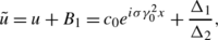
Using the DT, we obtain new exact solutions for the integrable generalization of the NLS equation (34):

(51)

where B ₁ is determined by (50).

• (I) For N=1, a direct calculation gives from (50) that

  

  According to the DT (39), we get an explicit solution for the integrable generalization of the NLS equation (34)

  

  (52)

  with

  $$\alpha_1=\frac{i\sigma\gamma_0^2+\sqrt{\Delta_1(\zeta _1)}+2i\zeta _1^2-2i\gamma_1\zeta_1\sigma\gamma_0^2c_0}{2i\zeta_1\sigma\gamma_0^2c_0-i\gamma_1\gamma_0^2+\sigma\gamma _1\sqrt {\Delta_1(\zeta_1)}-2i\sigma\gamma_1\zeta_1^2}e^{-i\sigma\gamma_0^2x},$$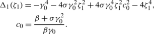
  

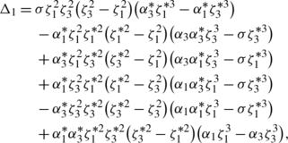
• (II) For N=2, we obtain from linear algebraic system (50) that

  

  (53)

  which is another explicit solution of (34), where

  
  
  $$\alpha_j=\frac{i\sigma\gamma_0^2+\sqrt{\Delta_1(\zeta _j)}+2i\zeta _j^2-2i\gamma_j\zeta_j\sigma\gamma_0^2c_0}{2i\zeta_j\sigma\gamma_0^2c_0-i\gamma_j\gamma_0^2+\sigma\gamma _j\sqrt {\Delta_1(\zeta_j)}-2i\sigma\gamma_j\zeta_j^2}e^{-i\sigma\gamma_0^2x},$$
  

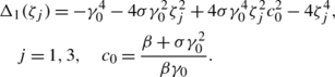
  Secondly, substituting the seek solution (47) of (34) into (3) and (4), their two basic solutions ϕ(ζ) and ψ(ζ) are taken as

  

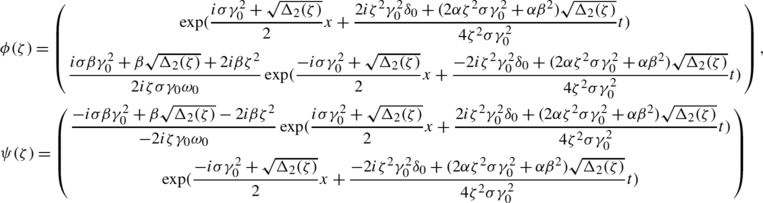  (54)

  in the view of (35), where

  

  Then (37) and (38) can be written as

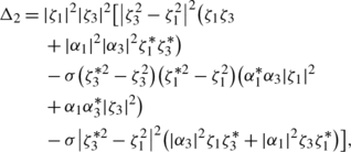
  $$\alpha_{2j-1}=\frac{i\sigma\beta\gamma_0^2+\beta\sqrt{\Delta _2(\zeta _{2j-1})}+2i\beta\zeta_{2j-1}^2-2i\gamma_{2j-1}\zeta_{2j-1}\sigma \gamma _0\omega_0}{2i\zeta_{2j-1}\sigma\gamma_0\omega_0-i\beta\gamma_{2j-1}\gamma _0^2+\sigma\beta\gamma_{2j-1}\sqrt{\Delta_2(\zeta _{2j-1})}-2i\sigma\beta \gamma_{2j-1}\zeta_{2j-1}^2}e^{-i\sigma\gamma_0^2x-i\sigma\delta_0t},$$

  (55)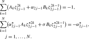
  

  (56)

  Using the DT, we obtain new exact solutions for the integrable generalization of the NLS equation (34):

  

  (57)

  where B ₁ is determined by (56).

• (I) For N=1, a direct calculation gives from (56) that

  

  According to the DT (39), we get an explicit solution for the integrable generalization of the NLS equation (34)

  

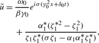  (58)

  with

  $$\alpha_1=\frac{i\sigma\beta\gamma_0^2+\beta\sqrt{\Delta_2(\zeta _1)}+2i\beta\zeta_1^2-2i\gamma_1\zeta_1\sigma\gamma_0\omega_0}{2i\zeta_1\sigma\gamma_0\omega_0-i\beta\gamma_1\gamma_0^2+\sigma \beta \gamma_1\sqrt{\Delta_2(\zeta_1)}-2i\sigma\beta\gamma_1\zeta _1^2}e^{-i\sigma\gamma_0^2x-i\sigma\delta_0t},$$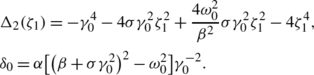
  

• (II) For N=2, we obtain from linear algebraic system (56) that

  

  (59)

  which is another explicit solution of (34), where

  
  
  $$\alpha_j=\frac{i\sigma\beta\gamma_0^2+\beta\sqrt{\Delta_2(\zeta _j)}+2i\beta\zeta_j^2-2i\gamma_j\zeta_j\sigma\gamma_0\omega_0}{2i\zeta_j\sigma\gamma_0\omega_0-i\beta\gamma_j\gamma_0^2+\sigma \beta \gamma_j\sqrt{\Delta_2(\zeta_j)}-2i\sigma\beta\gamma_j\zeta _j^2}e^{-i\sigma\gamma_0^2x-i\sigma\delta_0t},$$
  

4 Conclusions

The integrable generalization of the NLS equation models the propagation of nonlinear light pulses in optical fibers when certain higher-order non-linear effects are taken into account. Therefore, the study of explicit solutions for this equation is interesting and significant. The present work is devoted to a study for the integrable generalization of the NLS equation by means of the DT. In the foregoing sections, we have given an approach to construct a DT for the integrable generalization of the coupled NLS equation based on a gauge transformation between the corresponding spectral problems. A DT for the integrable generalization of the NLS equation is obtained through the reduction technique. As applications of DT, two classes of new explicit solutions for the integrable generalization of the NLS equation are given explicitly.

References

Fokas, A.S.: On a class of physically important integrable equations. Physica D 87, 145–150 (1995)
Lenells, L.: Exactly solvable model for nonlinear pulse propagation in optical fibers. Stud. Appl. Math. 123, 215–232 (2009)
Lenells, L., Fokas, A.S.: On a novel integrable generalization of the nonlinear Schrödinger equation. Nonlinearity 22, 11–27 (2009)
Lenells, L., Fokas, A.S.: An integrable generalization of the nonlinear Schrödinger equation on the half-line and solitons. Inverse Probl. 25, 115006 (2009)
Lenells, L.: Dressing for a novel integrable generalization of the nonlinear Schrödinger equation. J. Nonlinear Sci. 20, 709–722 (2010)
Matveev, V.B., Salle, M.A.: Darboux Transformations and Solitons. Springer, Berlin (1991)
Levi, D.: On a new Darboux transformation for the construction of exact solutions of the Schrödinger equation. Inverse Probl. 4, 165–172 (1988)
Gu, C.H., Zhou, Z.X.: On Darboux transformations for soliton equations in high-dimensional spacetime. Lett. Math. Phys. 32, 1–10 (1994)
Li, Y.S.: The reductions of the Darboux transformation and some solutions of the soliton equations. J. Phys. A 29, 4187–4195 (1996)
Geng, X.G., Ham, H.W.: Darboux transformation and soliton solutions for generalized nonlinear Schrödinger equations. J. Phys. Soc. Jpn. 68, 1508–1542 (1999)
Acknowledgements
This work was supported by National Natural Science Foundation of China (Project no. 11171312).
Author information
Authors and Affiliations
Corresponding author
Rights and permissions
About this article
Cite this article
Geng, X., Lv, Y. Darboux transformation for an integrable generalization of the nonlinear Schrödinger equation. Nonlinear Dyn 69, 1621–1630 (2012). https://doi.org/10.1007/s11071-012-0373-7
Received:
Accepted:
Published:
Issue Date:
DOI: https://doi.org/10.1007/s11071-012-0373-7