Integrated Co-evolution Model of Land Use and Traffic Network Design

Abstract

An integrated co-evolution model with the consideration of land use and traffic network design is proposed in this paper. In the suggested model, two kinds of economic agents are considered. On the one hand, the government makes the investment decision for the traffic network improvement based on the current traffic condition under the limited budget. On the other hand, households and companies will choose their locations according to the attraction of each traffic zone related to the road network accessibility and the housing price. Therefore, the land use is indicated by the population and employment distributions through the evolution process. Besides, the improvement of road capacity is modeled by a general bi-level programming of traffic network design. Simulation experiments show that the city will be more efficient and will have higher average accessibility for employment and population in the evolution process.

1 Introduction

With the rapid development of economy and urbanization, the contradiction between traffic demand and supply is constantly increasing. However, in the growth procession, traffic problems become more and more serious and gradually lead to the loss of city’s comprehensive functions. Among them, the urban traffic congestion has affected the city normal function and sustainable development severely. To alleviate these city ‘diseases’, the internal mechanism of urban evolution should be understood deeply, especially the relationship between land use and traffic network. Models of such interactions provide vital information to support many public policy decisions, such as land supply, infrastructure provision, and growth management (Zhang et al. 2009).

One of the complexities in modeling urban evolution is the interaction of land use and traffic system. Most previous efforts have been made to study transport and land use separately. Here, an integrated co-evolution model of land use and traffic network design has been given. Housing rental price which has significant effects on the residents’ location choice has been studied in the co-evolution process. Two kinds of economic agents (decision makers) have been confirmed and the interrelation between them has been studied deeply in the co-evolution process. Government departments optimize traffic network investment decision to minimize total travel cost, and the travelers’ route choice behavior was considered simultaneously after link capacity changed.

The rest of this paper is organized as follows. In the next section, a brief literature review is given. In section 3, the co-evolution process of land use and traffic networks is described detailed. Besides, some basic assumptions are given. Section 4 introduces the integrated co-evolution model of land use and traffic network design which consists of the traffic demand model, the traffic network investment model, the housing price distribution model and the land use model. Section 5 introduces the solution algorithm to solve this co-evolution model. Section 6 produces a set of simulation experiments to illustrate the application of the integrated co-evolution model. Then results and sensitivity of parameters are discussed. Section 7 provides conclusions and recommendations for future studies.

2 Brief Literature Review

As to the co-evolution of land use and traffic networks, there are five classes of model are explored.

Dynamics Evolution Models

The first dynamic model of the urban residential market was developed to explain the decay of the central locations in large old American cities (Anas 1978). It was found that the well-known static result of declining densities with distance from the center is shown to occur only under special conditions such as rising income levels. Dendrinos and Mullally (1981) presented a dynamical differential equation to describe the population dynamics. In 1985, they also proposed a predator–prey dynamic to simulate city evolution which considered cities as distinct units that compete with each other (Dendrinos and Mullally 1985).

Cellular Automata Models

Cellular automata (CA) models for city expansion simulation have proliferated along with the development of computer technology (Wagner 1997; Batty et al. 1999; Li and Yeh 2000; Batty 2007) because of their simplicity, flexibility and intuitiveness, especially the ability to incorporate the spatial and temporal dimensions in the processes. Yamins et al. (2003) presented a simulation model of road growing dynamics on a land use lattice that generates global features observed in urban transportation infrastructure. Li et al. (2003) built a model of simulating spatial urban expansion based on a physical process by applying CA model. In the model, they considered population density as an internal driving factor and economy as an external push on urban expansion. Lastly, a comprehensive review was presented to summarize the work in the early days (Santé et al. 2010). The review analyzed the CA models for the simulation of real-world urban process, classified CA models from the main characteristics of the models and analyzed their strengths and weaknesses.

Co-evolution Models

Levinson et al. (2007) firstly proposed a co-evolution model of land use and transportation. They found initially flat land uses become more concentrated while initially concentrated land uses become less so, and they tend to converge on the same hierarchical distribution, suggesting that a stable hierarchical distribution of land use may emerge from different initial conditions. In addition, a comprehensive review of modeling the growth of transportation network was presented (Xie and Levinson 2009a). Barthélemy et al. (2009) studied the influence that population density and the road network have on each others’ growth and evolution. They explicitly introduced the topology of the road network and analyzed how it evolves and interact with the evolution of population density. They found that accessibility issues pushing individuals to get closer to high centrality nodes lead to high density regions and the appearance of densely populated centers. Recently, Wu et al. (2013) studied the co-evolution process of private cars and public vehicles in the urban growth through establish a system dynamics model. They found that ignoring the co-evolution relation will lead to the disequilibrium development and cause the chaotic state of the urban transportation system eventually. To avoid the unsteadily development, a chaos control method was established.

Optimization Models

In previous studies, many scholars established optimization models to study the optimal land use structure, traffic networks and housing pricing distribution etc. Li et al. (2012) proposed a new model for investigating the effects of integrated rail and housing rental price on the design of rail line services in a linear monocentric city. They gave out the distribution of population, housing rental price when city system reached equilibrium. Then an analytical urban system equilibrium model for optimizing the density of radial major roads in a two-dimensional monocentric city was proposed (Li et al. 2013). They clearly stated there are four types of agents in the city system: local authorities, property developers, households and household workers.

Bid-rent Models

In recent years, the bid-rent model has been attracted much interest (Martínez 1992; Chang et al. 2006; Martinez et al. 2007; Ma et al. 2012; Bravo et al. 2010; Ma et al. 2013; Hurtubia et al. 2014). From the perspective of economics, it proposed rent estate combined with location options is assumed to be discrete and differentiated. Then the transactions are modeled as auctions. Martínez (1992) gave out the theoretical comparison of Alonso’s bid-rent theory and the discrete-choice random-utility theory. It is demonstrated that in perfectly competitive land markets these approaches are equivalent, therefore they should be understood as complementary rather than alternative. Chang et al. (2006) explored a bid-rent network equilibrium model which represents the relationship between transport and residential location. The relationship is examined in terms of the competition of decision-makers for location. This kind of model provides a new tool to study the interrelationship between land use and transport system.

In summary, many methods were explored to simulate the city evolution process and discovered the interaction between land use and traffic network. But there are many points to be improved. Firstly, previous studies paid little attention on the housing price which has significant effects on the residents’ location choice behavior in the co-evolution process of traffic network. Secondly, economic agents (decision makers) and their interrelationship in the co-evolution process of traffic network is always ignored in most previous studies. Moreover, most previous papers studied the city evolution without consider the increase of link capacity, or they simplified that government department made road investment not from the perspective of the whole traffic network but the single road.

To fill these gaps, in this paper, an integrated co-evolution model with the consideration of land use and a continuous network design problem (CNDP) is proposed. This paper makes three main contributions to the literature beyond previous studies (such as Levinson et al. 2007; Li et al. 2012) as following.

Firstly, the housing pricing is embedded in the model. We have studied housing rental price in the co-evolution process which has significant effects on the residents’ location choice. The step-by-step change of housing rental price in the co-evolution process has been given. Li et al. (2012) consider household’s residential location choices behavior is aim at modeling the design of rail line services which doesn’t affect the co-evolution process. Secondly, two kinds of economic agents (decision makers) have been confirmed and the interrelation between them has been studied deeply in the co-evolution process: (1) Government departments optimize traffic network investment decision to minimize total travel cost, and the travelers’ route choice behavior was considered simultaneously after link capacity changed; and (2) Households and companies choose their locations according to the attraction of each traffic zone which is related to the road network accessibility and the housing rental price. Besides, the traffic network investment model is proposed and GA is used to solve this model. From the simulation, some novel conclusions about the co-evolution of land use and traffic networks are given finally.

3 Model Framework and Assumptions

3.1 Model Framework

The components of integrated co-evolution model include four models, e.g., traffic demand model, traffic network investment model, housing price distribution model and land use model. The relationship among those models is illustrated in Fig. 1. As can be seen, there are two subjects in the co-evolution process: one is households and companies, and the other one is government departments. Generally, the location of households and companies determine the distributions of population and employment, which constitutes the urban land use structure. Meanwhile, the structure of urban land use affects the traffic demand, which further affects the road investment decision of the government department. Conversely, the road investment directly affects the link capacity of traffic network, which further affects the travel cost of different zones, and ultimately affects the distributions of accessibility and housing price. Finally, it will affect the location choice of households and companies. The step-by-step procedure and detailed model process (Input, Output, Subject and Model) are as follows:

Fig. 1

The co-evolution framework of land use and traffic networks

• Step 1: An initial distribution of population and employment in a city is given, namely initial land use pattern.

• Step 2: Traffic demand forecasting (Four-stage Method).

  The traffic demand model is transforming the information of population and employment into road traffic flow under the given road network by following the classic traffic planning method: traffic generation, traffic distribution, and traffic assignment.

  • Input: The distribution of population and employment.

  • Output: Link traffic flow on the traffic network.

• Step 3: Traffic network investment model (Continuous network design problem, CNDP)

  Government makes the investment decision for the traffic network improvement based on the current traffic condition under the limited fund.

  • Input: Link traffic flow on the traffic network, link capacity (before investment), etc.

  • Output: Increased link capacity (after investment), traffic cost between different zones, etc.

  Subject: Government department.

• Step 4: Accessibility.

  • Input: Distribution of population and employment, traffic cost between different zones, etc.

  • Output: Accessibility of every traffic zone.

• Step 5: Housing price distribution model.

  • Input: Traffic cost in every traffic zone, annual average household income, etc.

  • Output: Housing rental price in every traffic zone.

• Step 6: Land use model.

  • Input: Accessibility of every traffic zone, housing rental price in every traffic zone, Distribution of population and employment (before location choice), etc.

  • Output: Distribution of population and employment (after location choice).

  Subject: Household and company.

  Then go back to Step 2.

3.2 Assumptions

To facilitate the statement, the following basic assumptions are given in this paper.

• A1: The city concerned in this paper is assumed to be closed system which implies that the population and the total employments are fixed. These assumptions have been widely adopted in previous studies (see, Levinson et al. 2007; MacDonald 2009).

• A2: There are two types of agents in the economy: one is government departments, and another is households and companies. We assume that the investment decision of all individual roads in the city is decided by the same government departments. It spends all its available revenue at the end of a time period myopically, without saving it for the future. All households and companies (employment) are assumed to be homogeneous, which implies that the income level is identical for all households and companies. The objective of each household is to maximize its utility with its budget constraint (see, Li et al. 2012; 2013).

• A3: Most of business center, education agencies, financial company and other public service agencies will chose their locations near the downtown. We assume that the demand that commute to the downtown direction play the key role in their travel. Therefore, the average travel cost at the residential location is mainly affected by the demand close to the city center.

• A4: We assume that only the accessibility and the housing price affect the decision of location choice by households and companies. At the same time, business companies are more sensitive to the location and have a stronger ability to pay the rent (Alonso et al. 1964). Besides, we assume companies are less sensitive to the housing price than households in the process of location choice.

4 Integrated Co-evolution Model of Land Use and Traffic Network Design

4.1 Traffic Demand Model

In the beginning, there are a certain number of population and employments (jobs) in the network. Then, the travel demand is generated and is loaded into the traffic network eventually. Here, the traffic demand model is transforming the information of population and employment into road traffic flow under the given network by following the classic traffic planning method: traffic generation, traffic distribution, and traffic assignment.

We give out a simple traffic generation model to calculate the number of trip generation and trip attraction in different traffic zones. Both of them are generated from two parts: population (household) and employment (company). Assume that there is a simple linear relationship between the number of traffic generation, and the quantity of population and employment in traffic zone (Levinson et al. 2007).

$$ \begin{array}{cc}\hfill {O}_i={\xi}_1{E}_i+{\xi}_2{P}_i,\hfill & \hfill {D}_i={\psi}_1{E}_i+{\psi}_2{P}_i\hfill \end{array} $$

(1)

where O _i and D _i represent the number of trip generation or trip attraction in traffic zone i respectively, while E _i and P _i are the number of employments (jobs) and population (households) in the zone i. Besides, ξ ₁, ξ ₂ and ψ ₁, ψ ₂ are adjustable coefficients representing the traffic volume generated or attracted by unit employment and population, respectively.

The second step in traffic demand model is the traffic distribution. A doubly constrained gravity-based traffic distribution model is adopted to match both traffic generation and attraction of every OD pair based on a negative exponential function that assumes the traffic volume of different OD pair decreases with the travel time between them (Levinson et al. 2007; Zhang et al. 2009; Karoonsoontawong et al. 2015).

$$ {q}_{ij}={\varepsilon}_i{\partial}_j{O}_i{D}_jf\left({t}_{ij}\right) $$

(2)

where q _ij is the traffic volume from zone i to j. ε _i and ∂ _j are balancing coefficients which can be calculated through previous classic method (Xie 2008; Zhang et al. 2009), $\begin{array}{ccc}\hfill {\varepsilon}_i={\left[{\displaystyle \sum_j{\partial}_j{D}_j{e}^{-\varphi {t}_{ij}}}\right]}^{-1},\hfill & \hfill {\partial}_j={\left[{\displaystyle \sum_i{\varepsilon}_i{O}_i{e}^{-\varphi {t}_{ij}}}\right]}^{-1}.\hfill & \hfill f\left({t}_{ij}\right)={e}^{-\varphi {t}_{ij}}\hfill \end{array}$ is the travel cost function between zone i and j, and φ is a parameter which can be calibrated using the empirical data. t _ij is the travel time between zone i and j including two parts: intrazonal travel time within two traffic zones and the interzonal travel time between zones. It can be calculated by:

$$ {t}_{ij}=\left\{\begin{array}{c}\hfill \begin{array}{cc}\hfill {\displaystyle \sum_a\left({\zeta}_a^{ij}{u}_a\right)}+{t}_{m,i}+{t}_{m,j}\hfill & \hfill i\ne j\hfill \end{array}\hfill \\ {}\hfill \begin{array}{cc}\hfill {t}_{m,i}\hfill & \hfill i=j\hfill \end{array}\hfill \end{array}\right. $$

(3)

There are two parts in Eq. (3), the intrazonal travel time in the traffic zone i and j, and the interzonal travel time which is the summation of link travel cost along the shortest path between i and j. t _m,i is the intrazonal travel time in the zone i, which is proportional to the land use intensity. It can be calculated by a simple quadratic function ${t}_{m,i}={t}_m^0\left[1+{\left({Q}_i/\overline{Q}\right)}^2\right]$, where t ⁰ _m is a specified basic intrazonal travel cost. Q _i is the number of activities in zone i represented by E _i  + P _i describing the land use intensity of this traffic zone. Besides, $\overline{Q}$ is the average number of activities in traffic zones. In this paper, we define the number of activities is the summation of population and employment in a traffic zone. ζ ^ij _a is a 0–1 variable. If link a belongs to the shortest path from zone i to zone j, the value of ζ ^ij _a equals to 1. Otherwise, ζ ^ij _a  = 0.

The travel time on link a is the summation of two parts. ${u}_a=\frac{l_a}{v_a}+\frac{J_a}{x_a}\cdot \frac{1}{\eta }$ represents the travel time that a vehicle spends on link a including the actual travel time on link a and the equivalence time of monetary cost (toll) (Levinson et al. 2007). l _a , v _a , x _a and J _a is the road length, the average speed, the traffic flow and the collected revenue of link a, respectively. In addition, η is the average time value.

The third step of the traffic demand model is traffic assignment. After the two steps mentioned above, we can get the traffic volume of each OD pair. In this step, the classic user equilibrium model (UE) is adopted to describe travelers’ route choice behavior on the traffic network (Sheffi 1985). Therefore, we can get the link traffic flow through Frank-Wolfe algorithm (Frank and Wolfe 1956).

4.2 Traffic Network Investment Model

When the traffic flow is loaded on the links, the revenue model can be used to determine the price that the travelers must pay for using the road during a given time period which depending on the flow and the length of link (Levinson et al. 2007). The toll is approximately equivalent to a gas tax if it is proportional only to link length when government department allocates revenue back to links proportional to the amount of gas tax revenue those links generate (Levinson et al. 2006). To ensure two parallel and opposite one-way link a and b have the same condition, we always consider two links together (Levinson and Yerra 2006). The total revenue collected on both links by the agent can be calculated as:

$$ {J}_{a+b}=\tau {l}_a\left({x}_a+{x}_b\right) $$

(4)

where τ is the toll rate. x _a and x _b represent the traffic flow on link a and b.

Besides, the government will invest funds to maintain roads in their present useable condition. Generally, it is related to the link length l _a , traffic flow x _a and link free flow speed v _f,a . Therefore, the total cost on link a and b can be calculated by ${S}_{a+b}={l}_a{v}_{f,a}^{\sigma_2}\left({x}_a^{\sigma_1}+{x}_b^{\sigma_1}\right)$ (Levinson et al. 2007), where coefficients σ ₁ and σ ₂ are specified flow and speed powers. Therefore, the total revenue minus the cost is the available revenue which can be used by government departments to make investment as shown in Eq. (5).

$$ B={\displaystyle \sum_{a,b\in A}\left({J}_{a+b}-{S}_{a+b}\right)} $$

(5)

According to A2, it spends all the available revenue at the end of a time period without saving it for the future. Therefore, the target of government department is to minimize the total travel cost of traffic system by making investment policy under limited funding. On the other hand, from the user perspective, they always hope to minimize their own travel cost. This problem can be modeled as a typical CNDP under limited funding (Sun et al. 2014). Generally, a bi-level programming model can be used to describe this problem:

$$ \left(\mathrm{U}\right)\ \min\;F(Y)={\displaystyle \sum_{a\in A}{x}_a(y){t}_a\left({x}_a(y),{y}_a\right)} $$

(6)

$$ \mathrm{s}.\mathrm{t}.{\displaystyle \sum_{a\in A}{K}_a\Big(y{}_a\Big)}\le B $$

(7)

$$ \begin{array}{cc}\hfill {y}_a\ge 0\hfill & \hfill \forall a\in A\hfill \end{array} $$

(8)

$$ \left(\mathrm{L}\right)\ \min\;Z(X)={\displaystyle \sum_{a\in A}{\displaystyle {\int}_0^{x_a}{t}_a\left(\omega, {y}_a\right)}}d\omega $$

(9)

$$ \begin{array}{cc}\hfill \mathrm{s}.\mathrm{t}.{\displaystyle \sum_k{f}_k^{ij}}={q}_{ij}\hfill & \hfill \forall i\in \mathbb{R},j\in \mathbb{Z}\hfill \end{array} $$

(10)

$$ \begin{array}{cc}\hfill {f}_k^{ij}\ge 0\hfill & \hfill \forall i\in \mathbb{R},j\in \mathbb{Z},k\in {\mathbb{Q}}_{ij}\hfill \end{array} $$

(11)

$$ \begin{array}{cc}\hfill {x}_a={\displaystyle \sum_i{\displaystyle \sum_j{\displaystyle \sum_k{f}_k^{ij}{\delta}_{a,k}^{ij}}}}\hfill & \hfill \forall i\in \mathbb{R},j\in \mathbb{Z},k\in {\mathbb{Q}}_{ij}\hfill \end{array} $$

(12)

where A is the set of links in the network. ℝ is the set of origins. ℤ is the set of destinations. In addition, y _a represents the traffic capacity increment of link a. y = {…, y _a , …} is the set of link capacity increment which represents a decision scheme made by government departments. x _a is the traffic flow on link a. x(y) is the equilibrium flow defined by the lower level fixed demand static user equilibrium problem. q _ij is the traffic demand from origin i to destination j. f ^ij _k is the traffic flow of the k -th path from i to j. δ ^ij _a,k is a 0–1 variable. It equals to 1 if the link a belongs to the k -th path from i to j, otherwise it equals to 0. ℚ _ij is the set of all paths from i to j. t _a is the traffic impedance of link a which can be calculated according to the Bureau of Public Roads (BPR) function as $t{}_a={t}_0\left[1+\alpha {\left(\frac{x_a}{c_a}\right)}^{\beta}\right]$. Assume that the investment cost function K _a satisfies

$$ {K}_a\left({y}_a\right)={\gamma}_a{\left({y}_a\right)}^2 $$

(13)

where α, β and γ _a are specified coefficients. c _a is the traffic capacity of link a. t ₀ is the free flow travel time on link a.

Once the new link capacity is obtained, we used the log-linear model proposed by Zhang and Levinson (2005) to update the free flow speed of link a.

$$ {v}_{f,a}={\omega}_1+{\omega}_2 \ln {c}_a $$

(14)

where ω ₁ and ω ₂ are two coefficients in the log linear equation. The relationship between the free flow speed and the congested speed of a link can be determined by Eq. (15).

$$ {v}_{c,a}=\frac{v_{f,a}}{\left[1+\alpha {\left(\frac{x_a}{c_a}\right)}^{\beta}\right]} $$

(15)

Generally, the bi-level program mentioned above is always a NP-hard problem (Gao et al 2004). In the model, the upper level is non-convex and non-differentiable in which is defined by the lower level model. Algorithms for finding global optimal solutions are preferable to be used in solving it. In general, GA is a kind of efficient global search method and can then be used to determine the optimal solution of CNDP. However, the lower level program is a user equilibrium traffic assignment model, and Frank-Wolfe method can be used to solve it. We will introduce genetic algorithm to solve this bi-level model in section 5.

4.3 Accessibility

The accessibility of traffic zone indicates the collective performance of land use and transportation systems and describes how well that complex system serves its residents Geurs et al. 2004; El-Geneidy and Levinson (2006). In 1959, Hansen proposed the well-known definition of accessibility that the ability of people to reach the destinations to meet their needs and satisfy their wants (Hansen 1959). This definition has been long used in transportation planning, and reflects the difficult degree of getting employment (job) and population (resident) from a traffic zone.

In this paper we adopt the gravity-based method which is still the most widely used general method for measuring accessibility. Suppose an urban space is divided into n traffic zones or land use cells which contain both employments (jobs) and population (resident). The accessibility to employment and population can be calculated using a classic negative exponential measure in respectively with ${I}_{i,E}={\displaystyle \sum_{j=1}^n{E}_jf\left({t}_{ij}\right)}$, and ${I}_{i,P}={\displaystyle \sum_{j=1}^n{P}_jf\left({t}_{ij}\right)}$ El-Geneidy and Levinson (2006). f(t _ij ) is the travel cost function zone i and j which is the same as the doubly constrained gravity-based traffic distribution model in the section 4.1.

4.4 Housing Price Distribution Model

According to A2, each household is assumed to choose a residential location to maximize its own utility subject to the budget constraint. Following Beckman (1969; 1974) and Li et al., (2012; 2013), the following Cobb-Douglas form of the household utility function is adopted.

$$ \begin{array}{cc}\hfill U\left(z,g\right)={\theta}_1 \log z+{\theta}_2 \log g\hfill & \hfill {\theta}_1,{\theta}_2>0\hfill \end{array} $$

(16)

where U(z, g) is the utility function of households. θ ₁ and θ ₂ are specified positive constants and satisfies θ ₁ + θ ₂ = 1. z is the consumption of non-housing goods. g is the consumption of housing, measured in square meters of floor space.

Let x be the distance of a household’s residential from the CBD. The budget constraint for the household can be described as follows (Li et al. 2012):

$$ z(x)+R(x)g(x)=H-\phi (x) $$

(17)

where R(x) is the average rental price per unit of housing at location x, and H is the average household income. q _ij is the traffic volume from zone i to j per day. t _ij is the travel time from zone i to j (minutes). d(i), d(j) is the distance from zone i, j to the city center. ${\displaystyle \sum_{j\in {r}_j}{q}_{ij}},{r}_j=\left\{j\left|d(j)<d(i),j\in \mathbb{Z}\right.\right\}$ is the travel demand which commute to the downtown direction per day. $\frac{{\displaystyle \sum_{j\in {r}_j}{q}_{ij}t{}_{ij}}}{{\displaystyle \sum_{j\in {r}_j}{q}_{ij}}}$ is the average travel time per day in traffic zone i (minutes/day). η is the value of time (hour). ϕ(x) is the average annual travel cost at location x to medical treatment, education and other public service agencies, and it straightly affects housing price. According to A3, we can get

$$ \begin{array}{cc}\hfill \phi (x)={\phi}_i=365\cdot \eta \cdot \frac{1}{60}\frac{{\displaystyle \sum_{j\in {r}_j}{q}_{ij}t{}_{ij}}}{{\displaystyle \sum_{j\in {r}_j}{q}_{ij}}}=\frac{73}{12}\cdot \eta \frac{{\displaystyle \sum_{j\in {r}_j}{q}_{ij}t{}_{ij}}}{{\displaystyle \sum_{j\in {r}_j}{q}_{ij}}},\hfill & \hfill {r}_j=\left\{j\left|d(j)<d(i),j\in \mathbb{Z}\right.\right\}\hfill \end{array} $$

(18)

where i represents traffic zone which corresponds to location x, i ∈ ℝ. Then the utility maximization problem can be expressed as:

$$ \begin{array}{cc}\hfill \underset{x,g}{ \max}\hfill & \hfill U\left(x,g\right)={\theta}_1 \log \left(H-\phi (x)-R(x)g\right)+{\theta}_2 \log g\hfill \end{array} $$

(19)

It gives out the relationship between residential location x and housing rental price R (housing space g, etc.). In Li et al. (2012), the housing price and floor space functions are described with:

$$ R(x)={R}_0{\left(\frac{H-\phi (x)}{H-\phi (0)}\right)}^{\frac{\theta_1+{\theta}_2}{\theta_2}} $$

(20)

$$ g(x)=\frac{\left(H-\phi (0)\right){\theta}_2}{R_0\left({\theta}_1+{\theta}_2\right)}{\left(\frac{H-\phi (x)}{H-\phi (0)}\right)}^{-\cdot \frac{\theta_1}{\theta_2}} $$

(21)

where ϕ(0) is the intrazonal travel cost of CBD. R ₀ is the housing rental price of CBD which is proportional to the number of employment E ₀ which follows ${R}_0^{Step+1}={R}_0^{Step}\cdot {e}^{\frac{E_0^{Step+!}}{E_0^{Step}}-1}$, where R _0,t = 0 and E _0,t = 0 indicate the housing rental price and the number of employment in CBD at the initial co-evolution stage. Then we can obtain the optimal utility as following:

$$ {U}^{*}={\theta}_1 \log \left(\frac{\left(H-\phi (0)\right){\theta}_1}{\theta_1+{\theta}_2}\right)+{\theta}_2 \log \left(\frac{\left(H-\phi (0)\right){\theta}_2}{R_0\left({\theta}_1+{\theta}_2\right)}\right) $$

(22)

where R ₀ and ϕ(0) are constants at each step of co-evolution. That means when the residents’ location choice equilibrium state is reached, all residents in the monocentric city have the same utility regardless of their residential location and size of floor space. In the meanwhile, housing rental price R and floor space g are only relate to the residential location x. In general, the average housing rental price decreases and the average housing floor space per household increases with the increase of the travel cost, and vice versa.

The housing price distribution model gives out the relationship between residential location x and housing rental price R (housing space g etc.). The number of residents and employment at location x, namely the location of each traffic zone, will be discussed in the land use model.

4.5 Land Use Model

According to A4, the accessibility and the housing rental price are the only factors which affect location choice of households and companies. In this section, a land use model is developed to discuss the interrelationship. Our land use model contains both centripetal and centrifugal forces, namely a force of attraction and a force of repulsion. We assume population wants to be near employment, but far away from other residents. They always want to maximize available space and to avoid potential competitors for employment. In 2006, EI-Geneidy and Levinson found homebuyers pay a premium to live near jobs and away from competing workers El-Geneidy and Levinson (2006). In the meanwhile we assume companies want to be near other companies (employment) and people.

The following models are developed to calculate the attraction to population and employment of each traffic zone, respectively.

$$ \begin{array}{cc}\hfill {h}_{i,E}={I}_{i,E}^{\lambda_1}{I}_{i,P}^{\lambda_2}{e}^{-{\varsigma}_1\frac{R_i}{R_0}},\hfill & \hfill {h}_{i,P}={I}_{i,E}^{\lambda_3}{I}_{i,P}^{\lambda_4}{e}^{-{\varsigma}_2\frac{R_i}{R_0}}\hfill \end{array} $$

(23)

where λ ₁, λ ₂, λ ₃, λ ₄ and ς ₁, ς ₂ are coefficients indicating the positive or negative relationship between accessibility, housing rental price and land use. Obviously we have λ ₁, λ ₂, λ ₃, ς ₁, ς ₂ > 0 and λ ₄ < 0. According to A4, we assume companies are less sensitive to housing price than households in the process of location choice. Therefore, we can derive ς ₁ < ς ₂. According to the previous study in El-Geneidy and Levinson (2006), we can obtain λ ₃ = λ ₄.

Population and employment in the city are then reallocated across traffic zones at time period Step + 1 according to Eqs. (24–25). It basically in proportion to the desirability of each traffic zone at time period Step, except for the parameter μ introduced to indicate the reluctance for companies and people to move away from original location.

$$ \begin{array}{cc}\hfill {E}_i={\displaystyle \sum_{j=1}^n\left\{{E}_j^{Step}\frac{{\left({h}_{i,E}^{Step}\right)}^{\mu }}{{\displaystyle \sum_s{\left({h}_{s,E}^{Step}\right)}^{\mu }}}\right\}},\hfill & \hfill {P}_i={\displaystyle \sum_{j=1}^n\left\{{P}_j^{Step}\frac{{\left({h}_{i,P}^{Step}\right)}^{\mu }}{{\displaystyle \sum_s{\left({h}_{s,P}^{Step}\right)}^{\mu }}}\right\}}\hfill \end{array} $$

(24)

$$ \begin{array}{cc}\hfill {E}_i^{Step+1}={E}_i\frac{{\displaystyle \sum_{i=1}^n{E}_i^{Step}}}{{\displaystyle \sum_{i=1}^n{E}_i}},\hfill & \hfill {P}_i^{Step+1}={P}_i\frac{{\displaystyle \sum_{i=1}^n{P}_i^{Step}}}{{\displaystyle \sum_{i=1}^n{P}_i}}\hfill \end{array} $$

(25)

Eq. (25) are used to ensure the total number of employment and population are constant over time, where $\mu =\left\{\begin{array}{c}\hfill \begin{array}{cc}\hfill 1,\hfill & \hfill i=j\hfill \end{array}\hfill \\ {}\hfill \begin{array}{cc}\hfill <1,\hfill & \hfill i\ne j\hfill \end{array}\hfill \end{array}\right.$ _.

Housing price distribution model gives out the relationship between residential location x and housing rental price R. While the land use model shows the number of residents and employment at location x, namely the location of every traffic zone. Therefore, these two models together describe the households and companies’ location choice behavior.

There is a limitation in the part of household and company location choice behavior. Both microscopic model and macroscopic model have been used together. Originally, the household location choice is modeled via utility maximization with the Cobb-Douglas utility function. This utility maximization takes on a microeconomic approach. However, in the land use model, the reallocation of the population in the next year is model as a gravity type of model, which is macroscopic. But there are differences between utility maximization model and gravity model, they apply to different situation. Within each year/period, utility maximization is used to model household choice; whereas across the year, the relocation of residents is model based on the gravity model.

5 Solution Algorithm

In this section, a solution algorithm is proposed to solve the co-evolution model. The step-by-step procedure is as follows:

• Step 1 Initialization. A certain amount of E ⁰ and employment P ⁰ are distributed on the given traffic network. Determine the link traffic flow x _a (a ∈ A) according to the traffic demand model which is based on Eqs. (1)–(3). Set the iteration counter Step = 0.

• Step 2 According to Eqs. (4)–(5), we can calculate the available revenue B used by government departments to make investment. Then genetic algorithm was used to solve the upper level model of traffic investment in this paper. We take y _a (a ∈ A) as variables with real number encoding which constitute a chromosome. The solving steps of genetic algorithm are shown in Fig. 2. The brief summary of the genetic algorithm solves the CNDP is summarized as follows:

  Fig. 2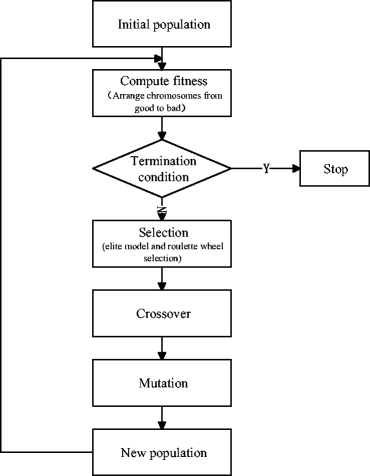

  

  The solving steps of genetic algorithm

  • Step 2.1 Initialization. At the beginning, we determine the probabilities of crossover (p _c ) and mutation (p _m ), the number of chromosome in the population (N), the maximum number of generations (M). And set the number of generations equal to zero (Gen = 0).

  • Step 2.2 We determine the fitness function according to the objective of the upper level model. Here the fitness function is $F(Y)={\displaystyle \sum_{a\in A}{x}_a(y)}{t}_a\left({x}_a(y),{y}_a\right)$. We take y _a (a ∈ A) as variables with real number encoding. Give out an initial population which is constituted of N random feasible solutions (chromosomes). Let Gen = 1.

  • Step 2.3 Take y = {…, y _a , …} (chromosome of the population) into lower model and then we can use the Frank-Wolfe method to solve it (Frank and Wolfe 1956). We can get the x _a (a ∈ A) corresponding to y = {…, y _a , …} and take it into the fitness function. Then we arrange all chromosomes from good to bad according to their corresponding fitness. If Gen = M, the chromosome which has the maximum fitness is the optimal solution, namely we can obtain every link capacity c _a (a ∈ A) after the investment. Then go to step 2.8. Otherwise go to Step 4.

  • Step 2.4 We obtain the next population according to the elite model and rank-based roulette wheel selection model (Xu et al. 2009).

  • Step 2.5 Crossover. The N chromosomes in the population are randomly divided into N/2 pairs. Assume V ₁ and V ₂ are two chromosomes and κ is a random number chosen from [0,1]. If κ < p _c , then the following crossover operations for V ₁ and V ₂ are performed. Otherwise no crossover operations are performed. Where s ∈ [0, 1] is a random number determining the crossover grade of those two chromosomes,

    $$ \left\{\begin{array}{c}\hfill {V}_1^{\hbox{'}}=s{V}_1+\left(1-s\right){V}_2\hfill \\ {}\hfill {V}_2^{\hbox{'}}=s{V}_2+\left(1-s\right){V}_1\hfill \end{array}\right. $$

  • Step 2.6 Mutation. Generate a random number κ for every chromosome. If κ < p _m , then the mutation operation for V is performed with V = V + m * L. Where m is a small positive constant and L is a random perturbation vector.

  • Step 2.7 Go back to Step 2.2.

  • Step 2.8 Update the free flow speed of every link v _f,a (a ∈ A) after its capacity changes according to Eq. (14) and calculate congested speed of a link v _c,a (a ∈ A) according to Eq. (15).

• Step 3 Determine the accessibility to employment I _i,E and population I _i,P from traffic zone i, respectively.

• Step 4 Update h _i,P and h _i,E of each traffic zone, respectively. Then update the number of employment E ^Step + 1 _i (i = 1, 2, …, n) and population P ^Step + 1 _i (i = 1, 2, …, n) of each traffic zone according to Eqs. (24) and (25). Terminate until population and employment in each traffic zone are almost unchanged. Otherwise, set Step = Step + 1 and go back to step 1.

As mentioned above, we can see that our co-evolution model integrating the traffic demand model, the traffic network investment model, housing price distribution model and the land use model.

6 Simulation Experiments and Analysis

6.1 Simulation Experiments

In this section, we use an example to illustrate the proposed model. The simulation experiments are based on a hypothetical metropolitan area where both the population and employment are distributed over the two-dimensional grid. This kind of simulation experiment has been widely adopted in previous studies (see, e.g., Li et al. 2003; Levinson et al. 2007; Santé et al. 2010). For simplicity, a city with 10 × 10 grid lattices is considered in this paper. Meanwhile, it stretches 20 km in both dimensions. Namely, it has 100 traffic zones and each traffic zone occupies one square kilometer. A total 100,000 people are living in the city, which is equivalent to an average of 1000 residents in each traffic zone. Total employment equals 100,000 as well which means every resident has a job opportunity. Two-way roads connect the centroids of each pair adjacent traffic zones, thus forming a 9 × 9 grid of road network as well, comprising 100 nodes and 360 links. Each link is 1 km in length with a free flow speed of 80 km/h, and a capacity of 800 veh/h in the first step.

As shown in Table 1, five sets of simulation experiments which adopt different road investment models and different initial distribution are conducted. The first experiment (UUL for short) makes road investment not from the perspective of the whole traffic network but the single road, government department charged on one link then spends all the revenue on this link (the link investment model can be seen in Levinson et al. (2007)). Namely they prefer to adopt link investment model rather than traffic network investment model in the co-evolution model. The second experiment (UUT for short) adopts the integrated co-evolution model proposed in this paper. In the meanwhile, each set of experiments was tested under the same initial conditions. These two experiments specify uniform land uses with both population and employment of each traffic zone equal to 1000. The third experiment (IUT for short) assumes a uniform distribution of population but a linear increasing distribution of employment so that zonal employment linear increases as the distance from the CBD to the edge of the city. Then the rest of experiments as described in Table 1.

Table 1 A set of simulation experiments

All parameters are used in the numerical example are listed in Table 2.

Table 2 List of parameters

Then a set of indexes was calculated to describe the collective properties for land use and traffic network.

• (1) Total travel cost is adopted to indicate the efficiency of traffic system which can be computed by $T={\displaystyle \sum_{a\in A}{x}_a}{t}_a\left({x}_a\right)$. As we can see, the purpose of transportation department is not only to provide fast and safe transportation, but also to provide an accessible and convenient transportation that meets the vital interests of the people and enhances quality of life today and in the future. The average accessibility to employment $\overline{I_E}={\displaystyle \sum_{i=1}^n{I}_{i,E}}/n$ and population $\overline{I_P}={\displaystyle \sum_{i=1}^n{I}_{i,P}}/n$ is adopted in this paper to indicate this function of transportation system in the co-evolution process.

• (2) Gini index is also adopted here to describe the uniformity of link capacity in traffic networks, the degree of spatial glomeration for population and employment which has been widely used in previous studies (Krugman 1991; Carlino and Chatterjee 2002). The more unevenly link capacity, distributions of population and employment, the higher value the Gini index is.

  $$ {G}_P=1-\frac{1}{n}\left(2{\displaystyle \sum_{i=1}^{n-1}\frac{{\displaystyle \sum_{j=1}^i{P}_j}}{P}}+1\right) $$

  (26)

  where G _P is the Gini index of population. P is the total number of population. Similarly, Gini index of link capacity G _c and employment G _E can also be calculated.

6.2 Results and Analysis

Figure 3 shows the distributions of employment and population when the city reaches a balanced state. It is found that all the simulation experiments have the similar distribution of employment and population in the end, namely the same balanced state. No matter what kinds of initial land use patterns, CBD will come into being spontaneously in the process of co-evolution, which has more companies and relatively fewer households. In particular, the number of companies decreases as the distance from CBD to the edge of city. But under the same condition, the number of population will increase firstly then decreasing. Most households are located at the edge of CBD rather than the city center. Clearly, we can see more jobs are located at CBD than the population which means companies are distributed closed to the city center.

Fig. 3

The distributions of employment and population

Figure 4 shows the distributions of activity Q and road capacity when the city reaches a balanced state. Clearly, the distribution is similar to Fig. 3. The reason is that large activity means a lot of traffic demand. Under limited road capacity, those roads become bottleneck for city development. Then in the traffic network investment part, the government department will make investment to improve the capacity.

Fig. 4

The distributions of activity Q and road capacity

Figure 5a indicates the change of urban total travel cost in those different co-evolution models. As we can see, total travel cost in those co-evolution models fluctuates wildly at the first several steps and then reaches a stable state. Obviously, the total travel cost in the experiment 1 is smaller than one in the experiment 2. It shows that under the same initial land use pattern the integrated co-evolution model in this paper has the smaller total travel cost than other co-evolution models. It means the traffic network investment model outperforms the link investment model. From Fig. 5b, we can see total travel cost in experiments 3–5 fluctuates wildly at the first several steps. It is because all of the experiments have uniform initial road capacity. The nonuniform land use pattern will make traffic congestion heavier. But it is improved after the traffic investment. In the end, experiments 2–5 with traffic network investment model under different initial land use patterns have the same total travel cost because the same stable state is reached.

Fig. 5

The total travel cost

Figure 6 shows the change of average accessibility to employment and population of these experiments. At the first step of co-evolution, an initial fixed traffic network is given out and we haven’t loaded traffic demand to the network, namely there is no traffic flow on the traffic network. Thus it has maximum average accessibility at the first step. With time going on, the average accessibility of different experiments decreasing and then reaches different balanced state. In the end, we can see experiments (UUT, IUT, UIT, IIT) with integrated co-evolution model in this paper have the better average accessibility to employment and population. The reason is that the government in the integrated co-evolution model made road investment not from the single road but from the whole traffic network perspective. Therefore, it decrease the travel cost and increase accessibility significantly.

Fig. 6

Average accessibility to employment and population

Figure 7 shows the Gini index of link capacity in all experiments increases slightly, but its value in experiments which adopt integrated co-evolution model is always bigger than the UUL model. It means that the integrated co-evolution model can improve the link capacity more centralized. The reason is that the traffic network investment model improves the capacity of targeted road. However, the link investment strategy in UUL model will improve road capacities causing the traffic bottleneck at the same time.

Fig. 7

Gini index of link capacity

From Fig. 8, we can see that the integrated co-evolution model makes employment and population more dispersed than the co-evolution model (link investment model). At the beginning of co-evolution process, experiments which have the same initial land use pattern have the same Gini index of employment and population. However, the integrated co-evolution model has a more dispersed employment and population distributions than the UUL model when it reached the stable state. In the end, all the experiments show that population is more dispersed than the employment.

Fig. 8

Gini index of employment and population

Figure 9 shows the change of housing rental price and housing space as the distance from CBD. The UUT model makes the rental price in CBD lower than the UUL model, but it improves housing prices in the suburbs. Specifically, when the distance from the CBD is less than 2.12 km, housing rents under UUT model are lower than those under UUL model. In the meanwhile it also can increase the housing space around the CBD but decrease housing space in the suburbs. When the distance from the CBD is less than 3.2 km, housing space under UUT model is bigger than those under UUL model.

Fig. 9

The distribution of housing rental price and housing space

6.3 Sensitivity Analysis

In this section, we analyze the sensitivity of θ ₁, θ ₂ which represents different consumption in the household utility function as Eq. (16). Household utility consists two parts: the utility of non-housing goods and the utility of housing. In the model, θ ₂ represents the importance of housing for households. For different people it has different value. This phenomenon has very important influence on the city spatial structure, such as the distribution of population and employment. Therefore we analyze the sensitivity of θ ₁, θ ₂ and give out the influence on the total travel cost, Gini index of employment (population, link capacity), housing rental price as followings.

From Fig. 10a we can see that if households more care about housing than non-housing goods, the total travel cost of urban traffic system will be deduced. Figure 10b indicates the size of θ ₂ has important influence on the road network structure. In the end urban traffic network capacity which has the largest θ ₂ is distributed more evenly than others. The larger size of θ ₂ makes the distribution of employment more concentrated but makes the distribution of population more dispersed as shown in Fig. 10e and f. From Fig. 10e and f, we can know the distribution of companies is more concentrated than population. Besides, the size of δ ₂ almost has no influence on average accessibility to employment and population as shown in Fig. 10c and d. Figure 10h shows the larger size of θ ₂ will make housing rental price decrease more significantly from CBD to the edge of the city. As a result, households may have a bigger housing space.

Fig. 10

Sensitivity analysis of θ ₂(θ ₁ + θ ₂ = 1)

7 Conclusions and Future Studies

This paper proposed a novel integrated co-evolution model of land use and traffic networks with considering CNDP and housing rental price. Initial symmetrical distribution of population and employment will become concentrate on the physical center of the area spontaneously. Then, the traffic congestion of CBD will become worse leading to the dispersion of people and employment. From the simulation, different initial distributions of land use have the similar distribution of employment and population, namely the same stable state and a stable monocentric city is formed over time. No matter what kinds of initial land use patterns, CBD will come into being spontaneously in the process of co-evolution, which has more companies and relatively fewer households. Besides, we find that most households are located at the CBD border rather than the city center. Furthermore, it is more reasonable that government department should make the road investment decision from the whole traffic network perspective.

How to measure the traffic carrying capacity in the co-evolution process and how to optimize land use and traffic networks under a given urban traffic carrying capacity should be paid much attractions in the future. Besides, the study combines with bid-rent model will be more meaningful in the coevolution of land use and traffic.

References

Alonso W (1964) Location and land use: toward a general theory of land rent [M]. Harvard University Press, Cambridge
Anas A (1978) Dynamics of urban residential growth [J]. J Urban Econ 5(1):66–87
Barthélemy M, Flammini A (2009) Co-evolution of density and topology in a simple model of city formation [J]. Netw Spat Econ 9(3):401–425
Batty M (2007) Cities and complexity: understanding cities with cellular automata, agent-based models, and fractals [M]. The MIT press, Cambridge
Batty M, Xie Y, Sun Z (1999) Modeling urban dynamics through GIS-based cellular automata [J]. Comput Environ Urban Syst 23(3):205–233
Beckmann MJ (1969) On the distribution of urban rent and residential density [J]. J Econ Theory 1(1):60–67
Beckmann MJ (1974) Spatial equilibrium in the housing market [J]. J Urban Econ 1(1):99–107
Bravo M, Briceno L, Cominetti R et al (2010) An integrated behavioral model of the land-use and transport systems with network congestion and location externalities [J]. Transp Res B Methodol 44(4):584–596
Carlino G, Chatterjee S (2002) Employment deconcentration: a new perspective on America’s postwar urban evolution [J]. J Reg Sci 42(3):445–475
Chang JS, Mackett RL (2006) A bi-level model of the relationship between transport and residential location [J]. Transp Res B Methodol 40(2):123–146
Dendrinos DS, Mullally H (1981) Evolutionary patterns of urban populations [J]. Geogr Anal 13(4):328–344
Dendrinos DS, Mullally H (1985) Urban evolution: studies in the mathematical ecology of cities [M]. Oxford University Press, Oxford
El-Geneidy AM, Levinson DM (2006) Access to destinations: development of accessibility measures[R]
Frank M, Wolfe P (1956) An algorithm for quadratic programming [J]. Nav Res Logist Q 3(1–2):95–110
Gao Z, Zhang H, Sun H (2004) Bi-level programming models, approaches and applications in urban transportation network design problems [J]. Commun Transp Syst Eng Inf 4(1):35–44
Geurs KT, van Wee B (2004) Accessibility evaluation of land-use and transport strategies: review and research directions [J]. J Transp Geogr 12(2):127–140
Hansen WG (1959) How accessibility shapes land use [J]. J Am Inst Planners 25(2):73–76
Hurtubia R, Bierlaire M (2014) Estimation of bid functions for location choice and price modeling with a latent variable approach [J]. Netw Spat Econ 14(1):47–65
Karoonsoontawong A, Lin DY (2015) Combined gravity model trip distribution and paired combinatorial logit stochastic user equilibrium problem [J]. Networks and Spatial Economics: 1–38
Krugman P (1991) Geography and trade [M]. The MIT press, Cambridge
Levinson D, Yerra B (2006) Self-organization of surface transportation networks [J]. Transp Sci 40(2):179–188
Levinson D, Xie F, Zhu S (2007) The co-evolution of land use and road networks [J]. Transportation and traffic theory: 839–859
Li X, Yeh AGO (2000) Modelling sustainable urban development by the integration of constrained cellular automata and GIS [J]. Int J Geogr Inf Sci 14(2):131–152
Li L, Sato Y, Zhu H (2003) Simulating spatial urban expansion based on a physical process [J]. Landsc Urban Plan 64(1):67–76
Li ZC, Lam WHK, Wong SC et al (2012) Modeling the effects of integrated rail and property development on the design of rail line services in a linear monocentric city [J]. Transp Res B Methodol 46(6):710–728
Li ZC, Chen YJ, Wang YD et al (2013) Optimal density of radial major roads in a two-dimensional monocentric city with endogenous residential distribution and housing prices[J]. Reg Sci Urban Econ 43(6):927–937
Ma XS, Lo HK (2012) Modeling transport management and land use over time [J]. Transp Res B Methodol 46(6):687–709
Ma XS, Lo HK (2013) On joint railway and housing development strategy [J]. Transp Res B Methodol 57(SI):451–467
Martínez FJ (1992) The bid-choice land-use model: an integrated economic framework [J]. Environ Plan A 24(6):871–885
Martinez FJ, Henriquez R (2007) A random bidding and supply land use equilibrium model [J]. Transp Res B Methodol 41(6):632–651
McDonald JF (2009) Calibration of a monocentric city model with mixed land use and congestion [J]. Reg Sci Urban Econ 39(1):90–96
Santé I, García AM, Miranda D et al (2010) Cellular automata models for the simulation of real-world urban processes: a review and analysis [J]. Landsc Urban Plan 96(2):108–122
Sheffi Y (1985) Urban transportation networks: equilibrium analysis with mathematical programming methods [J]. Transp Res Part A: Gen 20(1):76–77
Sun H, Gao Z, Szeto WY, Long J, Zhao F (2014) A distributionally robust joint chance constrained optimization model for the dynamic network design problem under demand uncertainty [J]. Netw Spat Econ 14(3–4):409–433
Wagner DF (1997) Cellular automata and geographic information systems [J]. Environ Plan B 24:219–234
Wu J, Xu M, Gao Z (2013) Coevolution dynamics model of road surface and urban traffic structure [J]. Nonlinear Dynamics: 1–8
Xie XJ (2008) Calibration method and comparison of gravity model [J]. Commun Stand 8:17–20
Xie F, Levinson D (2009) Modeling the growth of transportation networks: a comprehensive review [J]. Netw Spat Econ 9(3):291–307
Xu T, Wei H, Hu G (2009) Study on continuous network design problem using simulated annealing and genetic algorithm [J]. Expert Syst Appl 36(2):1322–1328
Yamins D, Rasmussen S, Fogel D (2003) Growing urban roads [J]. Netw Spat Econ 3(1):69–85
Zhang L, Levinson D (2005) Road pricing with autonomous links [J]. Transp Res Rec: J Transp Res Board 1932(1):147–155
Zhang L, Peng GX (2009) Simple method and application on calibration of the gravity model [J]. Technol Econ Areas Commun 11(1):106–108
Zhang L, Xu W, Li M (2009) Co-evolution of transportation and land use: modeling historical dependencies in land use and transportation decision-making[R]
Acknowledgments
This paper is partly supported by the National Natural Science Foundation of China (71322102, 71271024), the National Basic Research Program of China (2012CB725401), Program for New Century Excellent Talents in University (NCET-12-0764), the Fundamental Research Funds for the Central Universities (2015YJS093).
Author information
Authors and Affiliations
Corresponding authors
Rights and permissions
About this article
Cite this article
Li, T., Wu, J., Sun, H. et al. Integrated Co-evolution Model of Land Use and Traffic Network Design. Netw Spat Econ 16, 579–603 (2016). https://doi.org/10.1007/s11067-015-9289-3
Published:
Issue Date:
DOI: https://doi.org/10.1007/s11067-015-9289-3