Stochastic automated search methods in cellular automata: the discovery of tens of thousands of glider guns

Abstract

This paper deals with the spontaneous emergence of glider guns in cellular automata. An evolutionary search for glider guns with different parameters is described and other search techniques are also presented to provide a benchmark. We demonstrate the spontaneous emergence of an important number of novel glider guns discovered by an evolutionary algorithm. An automatic process to identify guns leads to a classification of glider guns that takes into account the number of emitted gliders of a specific type. We also show it is possible to discover guns for many other types of gliders. Significantly, all the found automata can be candidate to an automatic search for collision-based universal cellular automata simulating Turing machines in their space-time dynamics using gliders and glider guns.

1 Introduction

The emergence of computation in complex systems with simple components is a hot topic in the science of complexity (Wolfram 2002). Uniform frameworks to study emergent computation in complex systems are cellular automata (Von Neumann 1966). They are discrete systems in which an array of cells evolves from generation to generation on the basis of local transition rules (Wolfram 1984).

The well-established problems of emergent computation and universality in cellular automata has been tackled by a number of people in the last 30 years (Banks 1971; Margolus 1984; Lindgren and Nordahl 1990; Morita et al. 2002; Adamatzky 1998) and remains an area where amazing phenomena at the edge of theoretical computer science and non-linear science can be discovered.

We aim to construct an automatic system for the discovery of computationally universal cellular automata. A link between universality and the presence of mobiles self-localized patterns of non-resting states, called gliders, have been shown by Conway and his collegues (1982). To prove the universality of an automaton called the Game of Life, they employed gliders and their generators called glider guns which, when evolving alone, periodically recover their original shape after emitting a number of gliders. Here, we are interested in the emergence of glider guns.

The search for gliders was notably explored by Adamatzky and his collegues with a phenomenological search (2006), Wuensche who used his Z-parameter and entropy (Wuensche 2005) and Eppstein.¹ Lohn and Reggia (1997), Ventrella (2006) and Sapin et al. (2004a, b, 2006) have searched for gliders using genetic algorithms (10). In this work, automated search methods are used to search for glider guns for different types of glider.

Starting with the afore mentioned searches, three search methods for glider guns are compared. The results of the used methods are discussed, the guns are fully described using an automatic classification scheme. The same approach is then applied to search for other types of gliders. The paper is arranged as follows: Sect. 2 describes other related works. Section 3 sets out the characteristics of the search methods. Then the characteristics of the guns that were found, are described in Sects. 4 and 5 sets out the classification of the glider guns. Section 6 considers other guns then the last section summarizes the presented results and discusses directions for future research.

2 Previous work

In this section, some previous works dealing with cellular automata are presented. Brief descriptions of some search methods are given. Then some previous works about evolutionary approaches to search for automata are presented. To finish, An evolutionary discovered automaton is presented.

2.1 Cellular automata

In Wolfram and Packard (1985), Wolfram studied ${\mathcal E,}$ a space of two-state 2D automata with a transition rule that takes into account the eight neighbours of a cell in order to determine its state in the next generation. Sapin et al. (in press) have studied the appearance of gliders in this space but the discovered gliders were unidirectional. The scheme of demonstration of universality of the Game of Life requires isotropic gliders. As our aim is the discovery of computationally universal cellular automata, the considered cellular automata are the isotropic ones: if two cells have the same neighbourhood states by rotations and symmetries, then these two cells take the same state in the next generation.

There are 512 different rectangular 9-cell neighbourhood states (including the central cell) as shown in Fig. 1.

Fig. 1

Neighbourhood states that are the same by rotations and symmetries

The neighbourhood states can be divided in two subsets of 256 neighbourhood states. The neighbourhood states with the central cell in state zero are in the first subset and the others are in the second subset. All these neighbourhood states can be put in 102 subsets of isotropic neighbourhood states as shown Fig. 2 for the first subset of 256 neighbourhood states.

Fig. 2

Subset of isotropic neighbourhood states

The first element of each subset of isotropic neighbourhood states is used to represent a rule of ${\mathcal I}$ as shown Fig. 3 by telling what will become of a cell in the next generation, depending on its subset of isotropic neighbourhood states.

Fig. 3

The squares are the 102 neighbourhood states describing an automaton of $\mathcal I.$ A black cell on the right of the neighbourhood state indicates a future central cell

There are 102 subsets of isotropic neighbourhood states, meaning that there are 2¹⁰² different automata in ${\mathcal I}$ including the Game of Life that is outer totalistic i.e. the state of its cell in the next generation is determined by its state in current generation and the sum of the states of its eight neighbours. The subset of ${\mathcal I}$ of outer totalistic automata is composed by only 2⁹⁺⁹ = 262,144 elements. The elements of this set have been studied in detail and only the Game of Life has been proven computationally universal (Wolfram 1985, 2002; Heudin 1996).

2.2 Search methods

In order to search for universal automata, we have examined the search methods such as Monte Carlo, tabu search (Golver 1986) and evolutionary algorithms (EAs) (Holland 1975), as briefly described here.

The Monte Carlo method consists solely of generating random solutions and testing them.

Tabu search traverses the solution space by testing mutations of an individual solution. Tabu search generates many mutated solutions and moves to the best solution of those generated. In order to prevent cycling and encourage greater movement through the solution space, a tabu list is maintained of partial or complete solutions. It is forbidden to move to a solution that contains elements of the tabu list, which is updated as the solution traverses the solution space.

The class of computer search techniques known as EAs is being increasingly used in the design of complex systems. Populations of computer data structures encoding solutions to a given problem are manipulated using genetics-inspired mechanisms, under the influence of a selection pressure, to search for “fit” solutions. Example applications include data mining, time series analysis, scheduling, process control, robotics and electronic circuit design. EAs can be used for the design of computational resources in a way that offers substantial promise for application in complex systems since the algorithms are almost independent of the medium in which the computation occurs. Importantly, they do not need to directly manipulate the material to facilitate learning and hence the task itself can be defined in a fairly unsupervised manner. In contrast, most traditional learning algorithms use techniques that require detailed knowledge of and control over the computing substrate involved. In this paper we demonstrate the utility of EAs to discover glider guns within cellular automata.

2.3 Evolving cellular automata

Previously, several good results from the evolution of cellular automaton rules to perform some useful tasks have been published. After Packard (1988), Mitchell et al. (1993, 1994; Hordijk et al. 1998; Das et al. 1995) have investigated the use of evolutionary computing to learn the rules of uniform one-dimensional, binary cellular automata. Here a Genetic Algorithm produces the entries in the update table used by each cell, candidate solutions being evaluated with regard to their degree of success for the given task—density and synchronization. More recently, these tasks were also studied by Wolz and de Oliveira (2008).

Sipper (1997) has presented a related approach, which produces non-uniform solutions. Each cell of a one or two-dimensional cellular automata is viewed as a genetic algorithm population member, mating only with its lattice neighbours and receiving an individual fitness. Sipper shows an increase in performance over Mitchell et al.’s work, exploiting the potential for spatial heterogeneity in the tasks. Koza and his collegues (1999) have also repeated Mitchell et al.’s work, using Genetic Programming (Koza 1992) to evolve update rules. They report similar results.

2.4 Evolutionary discovered automaton

In Sapin et al. (2004a, b), in order to find computationally universal automaton, Sapin et al. used an evolutionary algorithm to find in ${\mathcal I}$ a subset of automata accepting gliders. One of the most commonly found gliders, named G, is shown in Fig. 4.

Fig. 4

Glider

This glider can be used for collision based computing (Sapin et al. 2004a, b) as logic gates can be simulated thanks to collisions of this glider.

Another glider, exhibited by the automaton of Fig. 3 called R, is emitted by a gun shown in Fig. 5.

Fig. 5

Glider gun and glider of the automaton R

This automaton is chosen on which attempts are made to demonstrate its universality. A combination of guns allow the simulation of a NAND by this automaton. The ability to create and assemble NAND gates into any logic circuit is then used to simulate a cell of the Game of Life as shown Fig. 6.

Fig. 6

Simulation of a cell of the Game of Life

The simulation of the Game of Life is then shown by carrying out a tilling of a surface with the identical simulation of cells as a proof that R is universal in the Turing sense, since the Game of Life was shown to be able to implement registers (Berlekamp et al. 1982).

3 Search methods for glider guns comparison

This section describes the search for glider guns. To compare the parameters of the search methods, glider guns that emitting the glider G shown Fig. 4 are searched for. The first search method is an evolutionary algorithm. Monte Carlo algorithm and tabu search are also used as benchmark.

3.1 Evolutionary algorithm

The parameters of the evolutionary algorithm are described here:

• Fitness function. The choice of the fitness function is perhaps the greatest difficulty with this problem. Lohn and Reggia (1997) have chosen a multiobjective function, Ventrella (2006) employed a particle swarm (Kennedy and Eberhart 1995) interacting with the cellular automata and Sapin et al. (in press) used an image-filtering to detect structures for measuring fitness.

  To find guns, the fitness function can evaluate the configuration of cells or the transition rule of automata. Cellular automata are highly sensitive to initial configuration of cells (Urfas et al. 1997) so the configuration of cells has been considered too difficult to evaluate by a fitness function. Thus the fitness function evaluates only the transition rule of each automata. To evaluate the transition rule, inspired by Sapin et al. (in press), a random configuration of cells is evolved by the tested automaton. The idea is to optimize the number of gliders and to prevent the configuration of cells from expanding. Then two fitness functions have been tried:

  • First fitness function

    After the evolution of the configuration of cells, the presence of gliders G is checked by scanning the result of the configuration of the cells. The value of the fitness function is the number of gliders that appeared divided by the total number of cells.

  • Second fitness function

    After the evolution of the configuration of cells, the presence of gliders G is checked by scanning the result of the configuration of the cells. The size of the biggest square S without cells in the evolved configuration of cells is computed. The value of the fitness function is the multiplication of the number of gliders that appeared by the size of the square S.

• Initialization. The search space is the set ${\mathcal I}$ described in Sect. 2. Cell-state transition table can describe an automaton of this space. An individual is an automaton coded as a bit string of 102 Booleans representing the values of a cell at the next generation for each neighbourhood state. The 102 bits of an automaton are divided into two subsets. The first subset, called the invarious subset, is the neighbourhood states used by the glider G and their values are determined by the evolution of this glider. The process that determines these neighbourhood states is detailed for the glider G in the Fig. 7. The other neighbourhood states are in the second subset, called the unused subset, and are initialised at random. The population size is 100 individuals.

  Fig. 7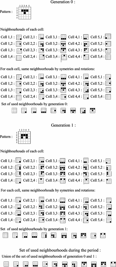

  

  Detail of the construction of set of neighbourhood states that are used by a glider

• Genetic operators. The mutation function simply consists of mutating one bit among the second subset of the 102 bits. The rates 1, 5 and 10% are tried, together with three crossover operators.

  • No crossover

    The genetic algorithm is tried without crossover.

  • Central point

    A single point crossover with a locus situated exactly on the middle of the genotype is tried.

  • Random point

    A last kind of recombination is tried with a single point crossover with a locus randomly situated.

    A linear ranking selection and a binary tournament selection of size 2 are tried.

• Evolution engine. An elitist strategy in which the best half of population is kept and a non-elitist strategy in which the new population is made of only children are tried.

• Stopping criterion. The presence of a glider gun is continuously checked. The test is inspired by Bays’ test (1987) and also used in Sapin et al. (2003). After the evolution of the random configuration of cells, each pattern is isolated and tested in an empty universe. If a pattern P reappears at the same place with gliders around then the pattern P is a glider gun. When a glider gun is found the algorithm stops.

  The value of the fitness function and the generation of the best rule are memorized. If after 10 new generations the algorithm has not found a better rule the algorithm stops.

  Thanks to these stopping criteria, an execution of the algorithm stops after an average of 38 generations.

3.2 Monte Carlo method

In 1 million randomly generated automata, the presence of glider guns after the evolution of a random configuration of cells has been tested. The test is the one used for the stopping criterion of the algorithm described in Sect. 3.1. There are not any guns found by this method.

3.3 Tabu search

The two fitness functions of the evolutionary algorithm are tried for this algorithm.

A random automaton A is generated, the fitness function measures the performance of this automaton.

All the automata obtained by mutating one bit among the unused subset, as described Sect. 3.1, are tested by the fitness function. The best one who is not in a list L of the last chosen automaton is chosen to become the new automaton A. The sizes of 10, 100 and 1000 are tried for the list L. The presence of glider guns is checked in all the tested automata.

The algorithm stops when the best automaton, among the automata obtained by mutation, that is not included in the list L is not better than the current automaton. With this stopping criterion, an execution of the algorithm stops after an average of 49, 42 and 35 generations depending on the size of the list L.

3.4 Discussion

For each of the values of the parameters, the number of executions which find a gun are shown in Table 1.

Table 1 Number of executions from a total of 100 per experiment that find a gun under a given combination of parameters or operators

The best parameters for the evolutionary algorithm, among the tested ones, are a mutation rate of 1, a non elitist strategy, a tournament selection, a central crossover and the second fitness function.

The good results of the central crossover can be explained by the fact that the first 51 neighbourhood states determine the birth of cells, while the other 51 determine how they survive or die. The elitist strategy that kept half of the population is worse than the non-elitist strategy. An elitist strategy that just kept one parent could however be tried.

The results of a Monte Carlo algorithm and tabu search, presented as benchmarks, are not as good as the evolutionary approach. The results of the EAs without crossover are about the same as the tabu search.

With the best parameters, as noted above, the average variation of the best value of the fitness function for 100 executions is shown Fig. 8.

Fig. 8

Average variation of the best fitness for 100 executions with the best parameters

The evolutionary algorithm with these parameters has been chosen to obtain the glider guns described in the next sections.

4 Best algorithm results

The results of the evolutionary algorithm for the glider G shown in Fig. 4 are described here as the number of glider guns that were found is set out.

In order to determine how many different glider guns were found, an automatic system that determines if a gun is new is required. At least two criteria can be used:

• Shapes of guns.

• Sets of used neighbourhood states.

The shapes of guns are not taken into account because there are an infinite number of guns with different shapes, as shown by the gun of Fig. 9 for which the central line can be arbitrary long.

Fig. 9

A gun

So, in order to determine if a gun is new, the set of neighbourhood states used by the given gun are compared to the ones of the other guns. For each gun and each neighbourhood state, three cases exist:

• The neighbourhood state is not used by this gun.

• The neighbourhood state is used by this gun and the value of the central cell in the next generation is 0.

• The neighbourhood state is used by this gun and the value of the central cell in the next generation is 1.

Two guns are different iff at least one neighbourhood state is not in the same case for the two guns.

Thanks to this qualification of different guns, through the experimentations, 20383 different glider guns were discovered. All these guns have emerged spontaneously from random configurations of cells. The 20383 guns can be found in Sapin (2007) in Life format.

The total number of different guns that could be found by this algorithm is unknown but the evolution of the percentage of new guns among the last 1000 different found guns is given by the Fig. 10.

Fig. 10

Evolution of the percentage of new guns among 1,000 different found guns

Suppose each gun has the same probability to be found.

Let N be the total number of guns that could be found by this algorithm. The probability of a gun found by the algorithm to be new would be 1−20383/N. The number of new guns among the last 1000 different found guns is 755. So the total number of guns that could be found by the algorithm could be estimated by N = 20383 * 1000/245 about 83196.

5 Classification

The first step to classify the glider guns is to determine the period of each gun. An automatic process, described in the first subsection, is required. The number of streams emitted during their period, used by the classification, is studied in a second subsection. The last subsection describes guns that have been found that emit one, two, three, four, six, eight, 12 and 14 gliders.

5.1 Period of guns

The period of a gun is the number of generations before the gun returns to its first shape after having emitted a number of gliders. To find the period of each gun the shape of the gun in the first generation is memorized and compared to the shape throughout the following generations. When the shape of the first generation is recovered, the algorithm checks if the other cells represent gliders. The period is found if the other cells only represent gliders.

The distribution of the periods of the found guns is shown Fig. 11.

Fig. 11

Distribution of the period of the found guns. Three other guns of period 62,74 and 243 are not shown on the graphic

The most common period is 18. The odd periods are the most common because most of the guns found recover a symmetric of their original shape after half of their period has ellapsed. The lowest found gun period is seven, a seven period gun is shown in Fig. 13. A lower gun period can not be found because the gliders of a stream emitted by a six period gun would not be sufficiently spaced. The gun found with the highest period, shown Fig. 29, emits 14 gliders during a period of 243 generations.

5.2 Number of emitted gliders

In order to know the number of emitted gliders for each gun, the following process is applied:

• The given glider gun evolves during its period.

• The cells of the glider gun are turned to 0.

• The number of gliders is counted.

The cells of the given glider gun are turned to 0 because gliders can be recognized in the shape of some guns as in the synchronous not lined up two-stream gun of Fig. 14.

The distribution of the number of guns found emitting n gliders during a period is shown Fig. 12.

Fig. 12

Distribution of the number of found guns emitting n gliders during a period

Guns that emit one, two, three, four, six, eight, 12 and 14 gliders were found. The most common number of emitted gliders is two. Most of this kind of guns recover a symmetric of their original shape after half of their period has ellapsed, after having emitted a glider. The guns emitting an odd number of gliders are not common as only guns emitting one and three gliders were found.

5.3 One stream guns

Two different types of streams can be emitted by a gun. If the period of the gun is a multiple of the period of the glider, the emitted gliders are in the same state during a generation of the automaton. If not the glider is not in the same state.

The period of the glider G is 2, so if the period of the gun is even, the gliders of the stream are in the same states. This kind of gun will be called Phased One Stream Gun or POS Gun and if the period is odd the gun is called Dephased One Stream Gun or DOS Gun. The two following subsections describe these two kinds of discovered guns.

5.3.1 POS gun

Figure 13 shows a POS gun with a emitted glider. The period of this gun is 10. The number of POS gun is 1,123 so 95% of one stream guns found are POS guns.

Fig. 13

A POS gun and a DOS gun

5.3.2 DOS gun

Among the 20383 discovered guns, there are 59 DOS Guns. Figure 13 shows a DOS gun of period 7.

5.4 Two stream guns

Two streams emitted by a discovered gun can be orthogonal or parallel. If the streams are parallel then they can be lined up or not lined up. So, there can be three cases:

• Orthogonal.

• Lined up.

• Not lined up.

During the period of a discovered gun, two streams can be emitted at the same time during the period of the gun or at different times; the terms asynchronous and synchronous streams will be used. At a given generation, two asynchronous streams can be in the same state, so these two streams are called phased streams, or in different states so they are called dephased streams. Three cases exist:

• Synchronous.

• Phased.

• Dephased.

The discovered guns that emit two streams can be classified in nine categories. Figures 14, 15 and 16 show one found glider gun of each category.

Fig. 14

From left to right: synchronous orthogonal two-stream gun, synchronous lined up two-stream gun, synchronous not lined up two-stream gun

Fig. 15

From left to right: phased orthogonal two-stream gun, phased lined up two-stream gun, phased not lined up two-stream gun

Fig. 16

From left to right: dephased orthogonal two-stream gun, dephased lined up two-stream gun, dephased not lined up two-stream gun

The numbers of two stream guns found by the algorithm of each type are shown in Table 2.

Table 2 Number of two stream guns of each type

5.5 Three stream guns

The three streams emitted by a discovered gun can be directed toward two cardinal directions or toward three cardinal directions.

The three emitted gliders can be in the same phase or in two different phases. The three streams are called phased streams or dephased streams.

During the period of a discovered gun, three streams can be emitted at the same time during the period of the gun, at two different times or at three different times, the following terms are used respectively:

• Asynchronous.

• Semi-asynchronous.

• Synchronous.

Among the 12 possible categories, guns were discovered in only four of them. Figure 17 shows one gun of these categories.

Fig. 17

From left to right: dephased, asynchronous and directed toward two directions three-stream gun, phased, asynchronous and directed toward two directions three-stream gun, phased, synchronous and directed toward three directions three-stream gun, phased, semi-asynchronous and directed toward three directions three-stream gun. The block of four cells in the shape of the last gun is an eater found by accident for this gun

The numbers of three stream guns found by the algorithm of each type are shown in Table 3.

Table 3 Number of three stream guns of each type

5.6 Four stream guns

The four streams emitted by a discovered gun can be directed toward the four cardinal directions or toward two cardinal directions. If the streams are directed toward the four cardinal directions then they can be lined up 2 by 2 or not lined up. So, there are three cases:

• Directed toward two cardinal directions.

• Directed toward four cardinal directions and lined up.

• Directed toward four cardinal directions and not lined up.

During the period of a discovered gun, four streams can be emitted at the same time, at two different times or at four different times, the following terms are used respectively:

• Asynchronous.

• Semi-asynchronous.

• Synchronous streams.

At a given generation, four streams can be in the same state or in two different states. The four streams are called phased streams or dephased streams.

Figures 18, 19, 20, 21, 22 and 23 show a gun from each of the 16 categories for which guns were found among the 18 possible categories of gun emitting four gliders.

Fig. 18

Phased and asynchronous four-stream guns. From left to right: directed toward two directions, four directions lined up and four directions not lined up

Fig. 19

Phased and semi-asynchronous four-stream gun. From left to right: directed toward two directions, directed toward four directions lined up and directed toward four directions not lined up

Fig. 20

Phased and synchronous four-stream guns. From left to right: directed toward two directions, four directions lined up and four directions not lined up

Fig. 21

Dephased and asynchronous four-stream guns. From left to right: directed toward two directions, directed toward four directions lined up and directed toward four directions not lined up

Fig. 22

Dephased, semi-asynchronous four-stream gun. From left to right: directed toward two directions, directed toward four directions lined up and directed toward four directions not lined up

Fig. 23

Dephased, synchronous and directed toward four directions lined up four-stream gun

The numbers of four-stream guns found by the algorithm of each type are shown in Table 4.

Table 4 Number of four stream guns of each type

5.7 Six stream guns

Thirty eight 6-stream guns were found. These guns can be put in four types described below and shown Fig. 24.

• First type. The six gliders can be emitted at four different times and toward six directions. Two couples of gliders are lined up as shown Fig. 24 for one of the 10 guns of this type.

• Second type. The six gliders can be emitted at three different times. The six gliders are emitted two by two toward four directions. As shown Fig. 24 for one of the two guns of this type, four gliders are lined up.

• Third type. The six gliders can be emitted at two different times. For the 13 found guns of this type, a first group of three gliders are emitted at half of the period and the three other gliders at the end of the period. The six gliders are emitted three by three toward six directions. As shown Fig. 24 for one of these guns, two couples of gliders are lined up.

• Fourth type. The six gliders can be emitted at the same time. For the four guns of this type, the six gliders are emitted toward six directions. As shown Fig. 24 for one of these guns, two couples of gliders are lined up.

  The numbers of six-stream guns found by the algorithm of each type are shown in Table 5.

Fig. 24

From left to right: one six-stream guns of each four discovered types

Table 5 Number of six stream guns of each type

5.8 Eight stream guns

Sixty four 8-stream guns were found. These guns can be put in five types described below and shown figs 25 and 26.

• First type. The eight gliders can be emitted at six different times and toward six directions. Two couples of gliders are lined up as shown Fig. 25 for the only gun of this type.

• Second type. The eight gliders can be emitted at two different times, toward four different directions and all in the same phase. As shown Fig. 25 for one of the sixteen found guns of this type, there are two groups of four lined up gliders.

• Third type. For the five guns of this type, The eight gliders are emitted at two different times, toward eight different directions and four in the same phase as shown Fig. 25.

• Fourth type. The eight gliders can be emitted at four different times. The eight gliders are emitted toward four directions with two gliders by directions. One of the eight guns of this type is shown 25.

• Fifth type. The thirty four guns of this type are like the guns of the second type but only four gliders are in the same phase as shown Fig. 25 for one of the thirty four guns found of this type.

Fig. 25

From left to right: one eight-stream guns of the three first discovered types

Fig. 26

From left to right: one eight-stream guns of the two last discovered types

The numbers of eight-stream guns found by the algorithm of each type are shown in Table 6.

Table 6 Number of eight stream guns of each type

5.9 Twelve stream guns

Guns that emit 12 streams during their period are not very common among the 20383 guns discovered. There are only two types of these guns called 12-stream guns.

The first 12-stream gun, shown in Fig. 27, emits four gliders at generations 10, 21 and 26 and its period is 38.

Fig. 27

A gun that emits 12 streams during its period

The second 12-stream gun, shown in Fig. 28, emits four gliders at generations 4, 14 and 38 and its period is 39.

Fig. 28

Discovered gun that emits 12 streams during its period

5.10 Fourteen stream guns

Only one 14-stream gun, shown Fig. 29 has been found. The period of this gun is 266 and two gliders are emitted toward two opposite directions at each of the four following generations: 23, 133, 156 and 266. In the first other direction one glider is emitted at generations 89, 122, and 266 and to finish in the last direction one glider is emitted at generations 133, 222 and 225.

Fig. 29

A gun that emits 14 streams during its period

6 Glider gun emitting diverse gliders

Our approach has also been applied to search for guns emitting other types of gliders. Using the same parameters as in the previous section, guns have been searching for the 100 gliders found by the algorithm described in Sapin et al. (2003, 2004a, b). Ten executions of our evolutionary algorithm per glider allow us to find guns for 55 gliders as shown Figs. 30, 31, 32 and 33.

Fig. 30

Gliders of speed 1 for which guns have been searched for. The gliders with black line border around them are the one for which at least one gun has been found

Fig. 31

Gliders of speed 1/2 for which guns have been searched for. The gliders with black line border around them are the one for which at least one gun has been found

Fig. 32

Gliders of speed 1/3, 1/4, 1/5, 2/7 and 1/9 for which guns have been searched for. The gliders with black line border around them are the one for which at least one gun has been found

Fig. 33

Diagonal gliders for which guns have been searched for. The gliders with black line border around them are the one for which at least one gun has been found

The averages of guns found for diagonal gliders and orthogonal gliders of each speed and each period are shown in Table 7.

Table 7 The averages of guns found for diagonal and orthogonal gliders of each speed and each period

The highest average is for period 2 and speed 1/2 that is the same period and speed of the glider G of Fig. 34.

Fig. 34

Gun emitting gliders for which the most guns have been found

The glider for which the most guns have been found is shown Fig. 7.

We can see some shape similarities between these gliders and the glider G.

7 Synthesis and perspectives

This paper deals with the emergence of computation in complex systems with local interactions. Different search methods are tried to find glider guns, building on previous work shown in Sapin et al. (2003, 2004a, b).

In particular, the Monte Carlo method, the tabu search and the evolutionary algorithms are explored with different parameters. The best results are found for an evolutionary algorithm. The experimentation showed that crossover in the evolutionary algorithm plays a key role in the search process. Future work will consider other search techniques.

The algorithm succeeded in finding 20383 glider guns (Sapin 2007) for the glider of Fig. 4 and found eaters in some cases by accident as shown in Fig. 17. A classification of the guns is presented based on the number of emitted gliders. For 100 different gliders we found 55 guns. For most of these gliders, no glider gun was known before.

The emergence of this number of glider guns is a very surprising result as Resnick et al. claimed: “‘You would be shocked to see something as large and organized as a glider gun emerge spontaneously.”’ (Resnick and Silverman 1996). The existence of so many different glider guns shows that they are far more easy to find than Wolfram has claimed about glider guns “‘There are however indications that the required initial configuration is quite large, and is very difficult to find.” (Wolfram 1984). Thus the discovery of the emergence and existence of so many different glider guns represents a significant contribution to the theory of cellular automata and complex systems that considers computational theory.

Further goals can be to find all the glider guns the algorithm can find and to find fitness functions in future which will discover the classes of missing of guns. All these automata may be potential candidates for being shown universal automata thanks to an automatic system for the demonstration of universal automata that can be developed. Then, another domain that seems worth exploring is how this approach could be extended to automata with more than two states (Wuensche and Adamatzky 2008).

Future work could also be to calculate for each automaton some rule-based parameters, e.g., Langton’s lambda (1990). All automata exhibiting glider guns may have similar values for these parameters that could lead to a better understanding of the link between the rule transition and the emergence of computation in cellular automata and therefore the emergence of computation in complex systems with simple components.

References

Adamatzky A (1998) Universal dymical computation in multi-dimensional excitable lattices. Int J Theor Phys 37:3069–3108
Andre D, Koza JR, Bennett FH III, Keane MA (1999) Genetic programming III: Darwinian invention and problem solving. Morgan Kaufmann, San Francisco, CA
Banks ER (1971) Information and transmission in cellular automata. PhD thesis, MIT
Bays C (1987) Candidates for the game of life in three dimensions. Complex Syst 1:373–400
Berlekamp E, Conway JH, Guy R (1982) Winning ways for your mathematical plays. Academic Press, New York
Das R, Crutchfield JP, Mitchell M, Hanson JE (1995) Evolving globally synchronized cellular automata. In: Proceedings of the sixth international conference on genetic algorithms, pp 336–343
Glover F (1986) Future paths for integer programming and links to artificial intelligence. Comput Oper Res 13:533–549
Heudin JC (1996) A new candidate rule for the game of two-dimensional life. Complex Syst 10:367–381
Holland JH (1975) Adaptation in natural and artificial systems. University of Michigan
Hordijk W, Crutchfield JP, Mitchell M (1998) Mechanisms of emergent computation in cellular automata. In: Eiben AE, BSck T, Schoenauer M, Schwefel H-P (eds) Parallel problem solving from nature-V, vol 866. Springer-Verlag, London, UK, pp 344–353
Kennedy J, Eberhart C (1995) Particle swarm optimization. In: Proceedings of the 1995 IEEE conference on neural networks
Koza JR (1992) Genetic programming: on the programming of computers by means of natural selection. MIT Press, Cambridge, MA
Langton CL (1990) Computation at the edge of chaos. Physica D 42:12–37
Lindgren K, Nordahl M (1990) Universal computation in simple one dimensional cellular automata. Complex Syst 4:299–318
Lohn JD, Reggia JA (1997) Automatic discovery of self-replicating structures in cellular automata. IEEE Trans Evol Comput 1:165–178
Margolus N (1984) Physics-like models of computation. Physica D 10:81–95
Martinez GJ, Adamatzky A, McIntosh HV (2006) Phenomenology of glider collisions in cellular automaton rule 54 and associated logical gates. Chaos, Solitons & Fractals 28(1):100–111
Mitchell M, Hraber PT, Crutchfield JP (1993) Revisiting the edge of chaos: evolving cellular automate to perform computations. Complex Syst 7:89–130
Mitchell M, Crutchfield JP, Hraber PT (1994) Evolving cellular automata to perform computations: mechanisms and impediments. Physica D 75:361–391
Morita K, Tojima Y, Katsunobo I, Ogiro T (2002) Universal computing in reversible and number-conserving two-dimensional cellular spaces. In: Adamatzky A (ed) Collision-based computing. Springer-Verlag, London, UK, pp 161–199
Packard NH (1988) Adaptation toward the edge of chaos. In: Kelso JAS, Mandell AJ, Shlesinger MF (eds) Dynamic patterns in complex systems, pp 293–301
Resnick M, Silverman B (1996) Exploring emergence. http://llk.media.mit.edu/projects/emergence/
Sapin E (2007) http://uncomp.uwe.ac.uk/sapin/gun
Sapin E, Bailleux O, Chabrier JJ (2003) Research of a cellular automaton simulating logic gates by evolutionary algorithms. In: EuroGP03 Lecture Notes in Computer Science, vol 2610, pp 414–423
Sapin E, Bailleux O, Chabrier JJ (2004a) Research of complex forms in the cellular automata by evolutionary algorithms. In: EA03 Lecture Notes in Computer Science, vol 2936, pp 373–400
Sapin E, Bailleux O, Chabrier JJ, Collet P (2004b) A new universal automata discovered by evolutionary algorithms. In: Gecco2004 Lecture Notes in Computer Science, vol 3102, pp 175–187
Sapin E, Bailleux O, Chabrier JJ, Collet P (2006) Demonstration of the universality of a new cellular automaton. In: Adamatzky A et al (eds) IJUC 2(3):79–103
Sapin E, Bailleux O, Chabrier J (2007) Research of complexity in cellular automata through evolutionary algorithms. Complex Syst 17(3):231–241
Sipper M (1997) Evolution of parallel cellular machines. In: Stauffer D (ed) Annual reviews of computational physics, V. World Scientific, Singapore, pp 243–285
Urfas J, Rechtman R, Enciso A (1997) Sensitive dependence on initial conditions for cellular automata. Chaos Interdiscip J Nonlinear Sci 7(4):688–693
Ventrella JJ (2006) A particle swarm selects for evolution of gliders in non-uniform 2d cellular automata. In: Artificial Life X: proceedings of the 10th international conference on the simulation and synthesis of living systems, pp 386–392
Von Neumann J (1966) Theory of self-reproducing automata. University of Illinois Press, Urbana, IL
Wolfram S (1984) Universality and complexity in cellular automata. Physica D 10:1–35
Wolfram S (2002) A new kind of science. Wolfram Media, Inc., Illinois, USA
Wolfram S, Packard NH (1985) Two-dimensional cellular automata. J Stat Phys 38:901–946
Wolz D, de Oliveira PB (2008) Very effective evolutionary techniques for searching cellular automata rule spaces. J Cell Autom 3(4):289–312
Wuensche A (2005) Discrete dynamics lab (ddlab). http://www.ddlab.org
Wuensche A, Adamatzky A (2008) On spiral glider-guns in hexagonal cellular automata: activator-inhibitor paradigm. Int J Mod Phys C 17(7):1009–1026
Acknowledgements
The work was supported by the Engineering and Physical Sciences Research Council (EPSRC) of the United Kingdom, Grant EP/E005241/1.
Author information
Authors and Affiliations
Corresponding author
Rights and permissions
About this article
Cite this article
Sapin, E., Adamatzky, A., Collet, P. et al. Stochastic automated search methods in cellular automata: the discovery of tens of thousands of glider guns. Nat Comput 9, 513–543 (2010). https://doi.org/10.1007/s11047-009-9109-0
Received:
Accepted:
Published:
Issue Date:
DOI: https://doi.org/10.1007/s11047-009-9109-0