
Abstract
Video contents contain complex structures due to the variety of the components and events involved. For example, surveillance videos often record multi-object interactions and consist of various scales of motion detail; Web videos are composed of multimodal cues, and each cue generally consists of a variety of scales of information. Generally, video contents comprise two types of the combination of the inherent structures: multi-modality/multi-scale and multi-object /multi-scale. Therefore, in this paper, we propose a new framework for video content modeling, under which video contents are decomposed into multiple interacting processes by double decomposition that aims at each type of combination of structures. To model the resulting processes, we propose a method named double-decomposed hidden Markov models (DDHMMs). DDHMMs contain multiple state chains that correspond to the interacting processes. To make the switching frequency of states in each chain consistent with the scale of the corresponding process, a durational state variable is introduced in DDHMMs. The proposed method performs well in modeling the relations among the interacting processes and the dynamics of each. We discuss the appropriate features under the proposed framework and evaluate DDHMMs in two applications, human motion recognition and web video categorization. The experimental results demonstrate that the double decomposition enhances video categorization performance in both cases.
1 Introduction
In this paper we investigate the problems of video content categorization using dynamic stochastic models. The task of video content categorization is to classify the videos into different classes based on their contents. Many interesting systems, including videos, are composed of multiple interacting processes, and thus merit a compositional representation of two or more variables. This is typically the case for systems that have the structure both in time and space. The space structure generally includes two types: multi-channel and multi-scale. A system can be thus analyzed with decomposition into multiple components in terms of the specific structures. Such decomposition may reveal some valuable information inherent in the systems, e.g. dependencies among different components, while significantly decreasing the complexity.
Videos can be treated as a dynamic system incorporating auditory, visual and textual information. There exist three typical types of structures of space in video contents.
-
Multi-modality: Web videos consist of multiple modalities such as visual, auditory and textual data [2, 13]. Visual modalities may be further distinguished into finer ones, such as the color, texture, and interest point.
-
Multi-object: For some applications such as intelligent surveillance, the motions of multiple objects (e.g. persons) are the most cues to show the semantics of video contents. In this case, we usually focus on the interactions among multiple-objects.
-
Multi-scale: Video contents are described by a variety of cues on different spatial or temporal resolutions. For example, to the visual modality, color histograms of a whole frame usually change more slowly than local color statistics over local regions of frames. Figure 1 illustrates another multi-scale example in the human motion case.
Fig. 1 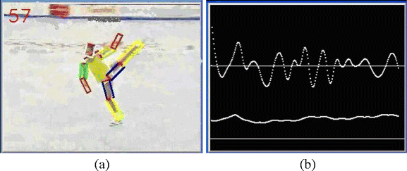
An illustration of the fact that human motions contain multiple scales of motion details. a skating, b the change of two kinds of features: the velocity of human’s whole body and the velocity of angle between two low limbs

Both multi-modality and multi-object cases are belong to the aforementioned multi-channel structure. In both multi-modality and multi-object structures, the components are generally symmetric and complementary in the representation of video contents, e.g. visual and auditory cues in multi-modality case, and the individual’s motions in multi-object case. Accordingly, we may decompose video contents into a number of interacting streams and model them using the same methodology for both cases. We refer to such decomposition as stream decomposition. As to the multi-scale structure, we decompose the video content into multiple sequences that locate on different temporal or spatial scales, and refer to this decomposition as scale decomposition. Stream and scale decompositions together comprise the double decomposition of video contents in this paper. Video contents may thus be analyzed by modeling such interacting stochastic processes derived by double decomposition.
Dynamic Bayesian networks (DBNs) [16] are powerful tools used to model interacting stochastic processes. DBNs are directed graphical models of stochastic processes, and each slice in a DBN contains one or multiple variables. As a simplest kind of DBNs, hidden Markov models (HMMs) [28] use a single state variable to encode all state information, and therefore require more parameters than other DBNs containing multiple variables to represent the same amount of information. Consequently, a number of variants of HMMs containing multiple variables have been proposed under the DBN framework, such as coupled HMMs (CHMMs) [1] and hierarchical HMMs (HHMMs) [6]. These methods have been widely used in applications ranging from speech recognition and video categorization to human-computer interaction.
In general, two or more types of structures usually coexist in video contents as described above, e.g. multi-object and multi-scale, or multi-modality and multi-scale. The double decomposition introduced above is thus necessary in video content modeling. To the best of our knowledge, the previous research has not handled the problem of video content modeling and categorization from the viewpoint of the double decomposition introduced above. Also, we don’t find a dynamic probabilistic model suitable to model the stochastic processes originated from the double decomposition effectively.
In this paper we propose a novel method, named double decomposed HMMs (DDHMMs), to model and categorize video contents from the viewpoint of the double decomposition. In DDHMMs, the state sequence is divided into multiple interacting Markov chains, each corresponding to one stochastic process derived from the double decomposition. The dependency among the chains shows the interactions of these components. To make the switching frequency of states consistent with the scale that the corresponding process locates on, an additional variable called durational state is introduced in DDHMMs to control the switching time of states. To summarize, we make the following contributions in this paper:
-
1.
We present a framework for video content modeling that decomposes video contents into multiple interacting processes through the stream and scale decomposition. This method of decomposition helps describe the structures inherent in video content, emphasizing the modeling of interactions among different processes and decreasing the complexity of dynamic systems.
-
2.
We model multiple processes derived under the framework described above using a new approach that we call DDHMMs. This approach is suited to model interactions among processes of different modalities/objects and those of different scales, as well as modeling the dynamics of each process.
The remainder of the paper is organized as follows. Section 2 reviews the related work. Section 3 analyzes the double decomposition for video contents. Section 4 introduces the proposed DDHMMs in detail. Sections 5 and 6 evaluate the performance of DDHMMs in applications of human motion recognition and web video categorization, respectively. Finally, Section 7 concludes this paper.
2 Related work
2.1 Multimodal fusion in video content analysis
Multimodal fusion is considered as an effective approach to both representing systems completely and tackling the curse of dimensionality problem. There is rich information from multiple channels in video contents, including visual, auditory, and textual data. One fusion method, known as early fusion, is to merge a variety of unimodal features into a single representation before classification [26]. Another fusion called late fusion learns classifiers directly from unimodal information, and then combines outputs of classifiers together. In the previous research, a variety of features have been used in early fusion or late fusion for video content analysis, such as the color, texture, object shape, interest point, text, and speech [26, 23, 25, 27]. Early fusion and late fusion differ in the way how the final decision is derived from the multimodal features. Snoek et al. [23] demonstrated experimentally that late fusion tended to provide a slightly better performance than early fusion in semantic video analysis. In addition to early and late fusion methods, there is a third fusion method, middle fusion, that combines multimodal features using one model or multiple coupled models [25].
In the literature, however, most research directly combines the extracted features with the fusion methods mentioned above, and don’t analyze the relationship among them deeply. Our method divides/decomposes the features into different components in terms of the structures in video contents introduced in Section 1, and fuses them together by a dynamic probabilistic model. More details will be shown in Section 3.
2.2 Dynamic Bayesian networks for dynamic system modeling
The dynamic Bayesian network is usually defined as a special case of singly connected Bayesian networks specifically aiming at the time series modeling, and has become an important tool for modeling dynamic systems [11, 10]. As a simplest kind of DBNs, HMMs [28, 9] have been widely used in many applications including speech recognition and human motion classification. The video content categorization using HMMs can be described as follows:
A generic hidden Markov model is illustrated in Fig. 2, where Q t and O t represent the hidden state and observation at time t, respectively. The parameters of an HMM are represented by \({\boldsymbol{\Theta} } = \{{\boldsymbol{\Pi}} ,\mathbf{A},\mathbf{B}\}\). The transition matrix A = (a ij ) is |Q| ×|Q| with \(a_{ij} = \Pr (Q_t = j|Q_{t - 1} = i)\), where |Q| denotes the number of states. The special case of time t = 1 is described by the initial state distribution \({\boldsymbol{\Pi}} = (\pi _i )\) with \(\pi _i = \Pr (Q_1 = i)\). B = (b j ( ·)) represents the complete collection of parameters for all observation distributions with \(b_j (O_t ) = \Pr (O_t |Q_t = j)\). In video content categorization with HMMs, O 1:T = { O 1 ,O 1 , ⋯ ,O T } denotes the observed sequence of feature vectors, such as the color histogram, texture and motion. For a class of video contents, an HMM is trained with \({\boldsymbol{\Theta}} ^\star = \arg \mathop {\max }\limits_{\boldsymbol{\Theta}} \Pr (O_{1:T} |\boldsymbol{\Theta} )\). Finally, a test video with observation sequence O 1:T can be categorized into the k-th class if \(k = \arg \mathop {\max }\limits_i \Pr (O_{1:T} |\boldsymbol{\Theta} _i ) \), where \(\boldsymbol{\Theta} _i\) is the model parameters trained on the i-th class of video data.

Hidden Markov models
HMMs use a single state variable to encode all state information, and thus require lots of parameters to model complex systems, and are prone to over-fitting when there are insufficient training data. Consequently, a number of variations of HMMs have been proposed for complex dynamic systems containing:
Multiple components with symmetric relationship
In this case, the separated components of systems usually symmetrically interact with each other. Brand et al. [1] proposed a coupled HMM to model such interacting components contained in human motions in surveillance videos, in which the multi-object structure of video contents was aimed at. In addition, some other methods, such as observation decomposed HMMs (ODHMMs) [12] and coupled hidden semi-Markov models (CHSMMs) [17], were also presented for the same issue. In ODHMMs, the observation is decomposed into a set of sub-observations for the multiple agents in the surveillance videos. The CHSMM is a variant of CHMMs in which a durational state is added to control the time when states switch. Nefian et al. [18] handled the speech recognition by conjoining visual and auditory cues, towards the multi-modality structure, with CHMMs.
Multiple components with different scales
Another group of methods aims at modeling multiple levels of information of complex dynamic systems that are generally on different scales. A representative model is hierarchical HMMs [6] that have been used in many data analysis applications including the speech recognition and human motion analysis. The layered HMM [20], a union of multiple separated HMMs, is another multi-level model often used to analyze complex sequences. Olivera et al. [20] modeled the motion details with different time granularity in office activities using the layered HMMs.
In addition to the two groups of methods described above, other methods have been presented in the literature. Huang et al. [10] used DBNs to detect events in soccer videos, in which each type of event was detected using one special DBN structure. In [3], Chen et al. proposed a layered time series model (LTSM), which combined HMMs and dynamic textures for gait recognition.
Base on the above overview, we find that most of the existing dynamic probabilistic models only aim at a single structure of multi-object, multi-modality, or multi-scale, and are not suited to handle the modeling of stochastic processes originated from the double decomposition of video contents.
3 The double decomposition of video contents
As briefly introduced in Section 1, video contents contain different structures including multi-object, multi-modality and multi-scale. In this section we analyze the decomposition of video contents into interacting processes in terms of these structures for two typical applications: human motion analysis in intelligent surveillance and web video content categorization.
3.1 Human motion analysis in intelligent surveillance
In the application of intelligent video surveillance, people usually focus on the motions of persons rather than the visual or auditory cues of the background. Multi-person motions (or interactions) consist of multiple individual’s motions that interact with each other. Therefore, we decompose human interactions into multiple coupled streams, each corresponding to an individual’s motion, which is the aforementioned stream decomposition. Each resulting individual’s motion contains various types of motion details that change at different speeds. For example, a walking human usually moves at a relatively steady speed with infrequently changing directions, while the angular velocity of the legs changes quickly. These motion details may be considered as locating on different temporal scales. Based on scale decomposition, we divide each individual’s motion into different scales of processes. As a result, an interaction of multiple persons is decomposed into a series of processes by the double decomposition, and is represented as follows:
where p l,c denotes the yielded process corresponding to the c-th person and l-th scale.
According to the strategy of decomposition for human interactions, the yielded process corresponding to an individual motion is not independent of others, and they affect on each other. That is, the relations between p l,c and p l,c′ need to be modeled for all l and \(c' \ne c\). Among the different scales, we consider that the processes on larger scales generally encode the dominant characteristics of dynamic systems, and play a more important role than those on the smaller scales. Furthermore, the interaction occurred between neighboring scales is stronger than between the other pairs. Figure 3 illustrates the double decomposition for a two-person interaction.

The double decomposition of a two-person interaction in surveillance videos, in which the trajectories and contours are considered as two scales of motion details
3.2 Web video content categorization
Web video contents consist of a variety of modalities, and in this paper we focus on the visual and auditory modalities. Both modalities are not independent of each other, and supplement each other when cooperatively representing the semantics of video contents. For example, in the task of soccer goal shot detection in sport videos, visual cues of the shot patterns and deafening audience applauds, which are both essential to the task, often occur simultaneously. Due to the approximation between the relationship among the components in multi-modality structure and that in multi-object case, we also refer to the division for the multi-modality structure as stream decomposition.
Each modality of video contents consists of a variety of attributes that can be employed for video representation, e.g. the color, texture and gradient in the visual modality, and Mel-frequency cepstral coefficients (MFCCs) and short time energy in the auditory modality. We notice that the commonly used features generally locate on different scales and represent the different characteristics of video contents. For the visual modality, the histogram of color and gradient in a whole frame generally changes slightly within a video shot due to the steadiness of scenes, and it thus changes with a low frequency throughout an entire video. Local visual features that are extracted from local regions (typically rectangles) of a frame usually change with high frequency in a video due to the possible foreground motions in scenes. For a further small scale, we may use the features of interest points, e.g. SIFT descriptors, to represent finer changes of background and foreground in video contents over time. The auditory modality also consists of a variety of features. Different from visual ones, multiple scales of auditory features are generally extracted based on the Wavelet or Fourier transform [24]. Figure 4 illustrates the double decomposition for the structure of multi-modality and multi-scale. Based on the decomposition/division, video contents can be transformed into a series of stochastic processes:
where p l,c denotes the process corresponding to the c-th modality and l-th scale.

The double decomposition of web video contents
Based on the aforesaid double decomposition in both applications, video contents are decomposed/divided into multiple interacting processes in terms of the structure of multi-channel and multi-scale. In both multi-modality and multi-object structures, the components originated from stream decomposition are generally symmetric and complementary as analyzed above. Therefore, we use the same methodology to model the stream decomposition for the two types of multi-channel structures. The components that are derived from the scale decomposition are usually asymmetric and describe the characteristics of video contents with different time granularity. To model the structure combination of both multi-modality/multi-scale and multi-object/multi-scale in video contents with a uniform framework of dynamic probabilistic models, we present a new method called double-decomposed HMMs.
4 Double-decomposed HMMs
In this section we introduce the double-decomposed HMMs that are used to model the double decomposition of video contents.
4.1 DDHMM definition
DDHMMs may be specified by the tuple:
In DDHMMs, \(\mathcal Q = \{Q^{l,c}\}\) and \(\mathcal O = \{O^{l,c}\}\) are the hidden state variables and observation variables, and \(\mathcal D = \{D^{h,c}\}\), called durational state, records the duration that the state Q h,c lasts, i.e., \(D_t^{h,c} = d\) represents that \(Q_t^{l,c} \) remains unchanged for the duration of d before its transit to a new state; c = 1,2, ⋯ , C is the stream index, both l = 1,2, ⋯ , L and h = 1,2, ⋯ , L − 1 are the scale indices, and L is the number of scales (or levels) in DDHMMs. Q l,c and D h,c take on discrete values { 1,2, ⋯ ,|Q l,c| } and { d|d ∈ ℕ ∪ { 0} }, respectively, where |Q l,c| denotes the number of values that Q l,c takes on, and ℕ denotes the set of natural numbers. Each time slice of DDHMMs consists of observation nodes \(O_t = (O^{1,1}_t,\cdots, O^{L,C}_t)\) and state nodes \(S_t = \{Q_t,D_t\} = \{(Q^{1,1}_t,\cdots, Q^{L,C}_t),(D^{1,1}_t,\cdots, D^{L-1,C}_t)\}\). Note that there is no durational state in the lowest level of DDHMMs. Figure 5 illustrates the proposed DDHMMs, in which Fig. 5a shows the relationship among hidden variables, omitting the duration states and observation variables for simplicity, and Fig. 5b shows explicitly the detailed structure of a state chain in Fig. 5a.

L-level double-decomposed HMMs
The transition matrix A is the complete collection of parameters that represent the probability of making transition from state \(Q^{l,c}_{t-1}\) to \(Q^{l,c}_{t}\) and contains the following elements:
In (4), \(Q^{l,c}_t\) does not change when \(D^{l,c}_{t - 1} > 0\). The special case of time t = 1 is described by the initial state distribution \({\boldsymbol{\Pi}} \) that contains the following elements:
for c = 1,2, ⋯ ,C. The distribution of durational state \(D^{l,c}_t\) is described by \(\mathbf P = \{p^{l,c}_{d|i}\}\) that is defined as follows:
If \(D_{t - 1}^{l,c} = d' > 0\), \(D_t^{l,c} = d' - 1\). From (4) and (6) we know that the durational state \(D^{l,c}_t\) controls the time when state \(Q^{l,c}_t\) transits. Finally, the observation distribution B = ( b i (·)) is modeled by Gaussian mixture models (GMMs) as follows:
where \(w^{l,c}_{im}\), \(\boldsymbol {\mu} ^{l,c}_{im}\), \(\boldsymbol {\Sigma}^{l,c}_{im}\) are the weight, mean vector, and covariance matrix of the m-th component respectively, \(M^{l,c}_i\) is the number of components of the GMMs for \(Q^{l,c}_t = i\), l = 1,2, ⋯ ,L, c = 1,2, ⋯ ,C. For simplicity, we let \(M^{l,c}_i = M_l\) for all c and i.
4.2 Model structure analysis
Suppose HMMs are generalized by letting the state be represented by a collection of state variables: Q 1,1, ⋯ ,Q l,c, ⋯ ,Q L,C, each of which takes on |Q| values. Given all the |Q|LC combinations of the states, placing no constraint on the state transition structure would result in a transition matrix of size |Q|LC×|Q|LC. Such an unconstrained system is equivalent to an HMM with |Q|LC states, and is unlikely to discover any interesting structures in the LC variables, as all variables are allowed to interact arbitrarily [8]. Therefore, we focus on DDHMMs in which the underlying the state transitions are constrained. The size of transition matrix of DDHMMs is reduced to approximately LC|Q|C + 1·|Q| (excluding the variable D l,c).
As is shown in Fig. 5a, nodes in DDHMMs are decomposed in two ways. The first is to decompose chains on the horizontal planes (referred to as levels) in the figure, which corresponds to the stream decomposition. The second is to decompose on vertical planes corresponding to scale decomposition, where a lower level in DDHMMs means a smaller scale. Within one level, the coupling structure of chains reflects the relationships of the multiple processes on the corresponding scale, which can be determined empirically or through model structure learning. Figure 6 shows three types of coupling of multiple state chains within the same level in DDHMMs. Scale decomposition results in the explicit interactions of processes among different scales. We consider that the processes on larger scales generally encode the dominant characteristics of dynamic systems and play a more important role than those on smaller scales. Furthermore, the interaction occurring between neighboring scales is stronger than that between the other pairs. As a result, in DDHMMs we only preserve those directed edges that are from one level of states to the immediately lower level (cf. Fig. 5). On each level, the frequency of state transition must be constrained to be consistent with the corresponding scale. To this end, a durational state D l,c is introduced to control the time when state Q l,c transits, l = 1,2, ⋯ ,L − 1. In the L-th level, the state duration implicitly follows exponential distributions without the direct constraint of durational states.

Three examples of coupling of state chains on the same level of DDHMMs with C = 5. In this figure, double-head arrows denote the coupling of two state chains
The double decomposition of state space in DDHMMs has several advantages. First, DDHMMs can formulate interactions among multiple streams and multiple scales contained in dynamic systems. Second, DDHMMs can represent multiple scales of information contained in the systems. Third, DDHMMs greatly reduce the dimensionality of feature, state and parameter spaces with double decomposition, decreasing the complexity of dynamic systems and making the model training and the inference more tractable.
4.3 The distribution of durational states
As is shown in (4) and (6), \(\mathbf P = \{p^{l,c}_{d|i}\}\) explicitly gives the probability that the duration of state \(Q^{l,c}_t\) equals d in the DDHMMs. A classic approach is to model the duration explicitly via the multinomial distribution [15]; However, its drawback is in the large number of free parameters needed, which requires more training data and incurs extra computation cost in both training and classification. Existing approaches to overcome this problem typically use a more compact parametric duration model. In general, the selected duration model should be simple for the high efficiency of computation. In addition, when the maximum duration length is large, the inference usually becomes very inefficient. Based on the above analysis, we use two types of duration models in our work.
4.3.1 Uniform distribution
The uniform distribution is a compact model with only two parameters: lower bounds and upper bounds. Its simplicity makes the inference on DDHMMs efficient. Considering the state Q l,c = i in DDHMMs, the lower and upper bounds are estimated as follows:
where \(d^{l,c}_{ik} \) is the duration that state Q l,c = i lasts given the k-th training sequence of length T k . The advantage of uniform distributions is that only a few parameters need to be estimated. However, when the maximal interval \(H^{l,c}=\max_i(u^{l,c}_i - l^{l,c}_i)\) is large, the inference on DDHMMs comes with a high computational load.
4.3.2 Discrete Coxian distribution
One problem with most distributions (including the uniform distribution) in the modeling of state durations is that inference complexity increases rapidly as the maximal interval increases. Discrete Coxian distributions, however, can effectively overcome this drawback [5].
Discrete Coxian distribution is a class of phase-type distribution, and the H cox-phase discrete Coxian distribution is defined as follows:
\(DCox({\boldsymbol{\nu }},{\boldsymbol{\lambda }})\) denotes the random variable obeying discrete Coxian distribution with parameters \(\boldsymbol{\nu }\) and \(\boldsymbol{\lambda }\), where \({\boldsymbol{\nu }} = \{ \nu _1 ,\nu _2 , \cdots ,\nu_{H_{\rm cox}}\}\), \(\sum\nolimits_{z = 1}^{H_{\rm cox} } {\nu _z } = 1\), \({\boldsymbol{\lambda }} = \{ \lambda _1 ,\lambda _2 , \cdots ,\lambda _{H_{\rm cox}}\}\), \(V_j =\sum\nolimits_{z = j}^{H_{\rm cox}} {X_z }\), and X z is the variable with geometric distribution Geom(λ z ). In fact, discrete Coxian distribution is equal to the distribution of the duration of a left-to-right Markov chain with H cox + 1 states numbered from 1 to H cox + 1, with the initial probability ν z and the self-transition probability λ z for state z, z = 1,2 ⋯ , H cox. The first H cox states represent the H cox phases, while the last one is absorbing and acts like an end state.
For the state Q l,c = i in DDHMMs, we let the corresponding durational state D l,c take on the values \(\{1,2,\cdots,H^{l,c}_{\rm cox}, \;'e'\}\) instead of { d|d ∈ ℕ ∪ { 0} } (cf. Section 3.1), where ′e′ denotes the end state. \(Q_t^{l,c}\) will transit when \(D_t^{l,c} = 'e'\). As a result, \(p^{l,c}_{d|i}\) in (4) is given by discrete Coxian distribution with the following parameters:
where O (k) (k = 1,2, ⋯ ,K) is the k-th sequence of length T k , and P 1 and P 2 denote the terms at t = 1, \(P_1 = \Pr(O^{(k)} ,Q^{l,c}_1 = i,D^{l,c}_1 = z|\Theta )\), \(P_2 = \Pr(O^{(k)} ,Q^{l,c}_1 = i|\Theta )\).
4.4 Model initialization
The parameter set Θ of DDHMMs must first be initialized before model training. Because learning methods based on the expectation maximization (EM) algorithm generally converge to a local optimum, the learning results of DDHMMs are dependent on the initial values of the model parameters.
Generally, the initial probability \(\boldsymbol{\Pi}\) and the transition probability A have little effect on learning results. Therefore, we initialize them with uniform distributions, and focus on the initialization of observation probability B and duration distribution P. We assume that observation probabilities can be initialized independently for different state chains in DDHMMs. To observation \(O_{1:T}^{l,c}\) associated with the l-th level and the c-th stream of DDHMMs, we firstly separate them into |Q l,c| (cf. Section 3.1) groups using k-means clustering algorithm, where each group corresponds to one discrete value of Q l,c. The i-th group corresponding to Q l,c = i is modeled using Gaussian mixture models. The parameters of GMMs are estimated using the EM algorithm, and the initialization results of observation probabilities are achieved. For the duration distribution P, we use \(\nu_{iz}^{l,c} = 1/H^{l,c}_{\rm cox}\) and \(\lambda_{iz}^{l,c} = 0.5\) for \(z = 1,2,\cdots,H^{l,c}_{\rm cox}\) when \(H^{l,c}_{\rm cox}\)-phase discrete Coxian distributions are used. If uniform distributions are used, we choose the initial values \(l^{l,c}_i = \min_k(1/T_k)\) and \(u^{l,c}_i = 1\) for i = 1,2, ⋯ , |Q l,c|.
4.5 Model inference and learning
As a special case of dynamic Bayesian networks, DDHMMs can be inferred and learned by the existing methods for DBNs [16].
In DDHMMs, \(S_t = \{(Q^{1,1}_t,\cdots, Q^{L,C}_t),(D^{1,1}_t,\cdots, D^{L-1,C}_t)\}\) and \(O_t = (O^{1,1}_t,\\\cdots, O^{L,C}_t)\) denote states and observations at time t, while S 1:T = (S 1 ,S 2 , ⋯ ,S T ) and O 1:T = (O 1 ,O 2 , ⋯ ,O T ) denote the state and observation sequences of length T, respectively. Given an observation sequence, the main task of inference on a model is to calculate the posterior probabilities \(\Pr(S_t |O_{1:T} ,\Theta ) \) and \(\Pr(S_t ,S_{t + 1} |O_{1:T} ,\Theta ) \), and the optimal state sequence \(S_{1:T}^\star\), where Θ denotes the parameter set of the model. In this paper, we compute the former with the interface algorithm [16], and the latter with the Viterbi-like algorithm [7]. The complexity of interface inference on DDHMMs is O(T·J (2L + 1)C), where \(J = \max_{h,c}(|D^{h,c}|, |Q^{h,c}|, |Q^{L,c}|)\), in which |D h,c| equals H h,c or \(H^{h,c}_{\rm cox}+1\) when a uniform distribution or a discrete Coxian distribution is used. For the HMM, CHMM, and HHMM with the same size of state space, the complexity is approximately O(T·J 4LC), O(T·J 4LC), and O(T·J (2L + 1)C), respectively. We observe that the complexity of inference on DDHMMs is approximate to HHMMs and lower than HMMs and CHMMs. In general, \(H^{h,c}_{\rm cox}\ll H^{h,c}\), thus discrete Coxian distribution can lead to computationally efficient inference. When L or C is large, the exact inference on DDHMMs is intractable due to the exponential inference complexity w.r.t. L and C. In this case approximate inference needs to be used. For example, if approximate inference based on Gibbs sampling is used, the computational complexity is \(O(T\cdot(\sum\nolimits_{l,c} {|Q^{l,c}|} + \sum\nolimits_{h,c} {|D^{h,c}| })\).
The aim of learning is to estimate the parameter set Θ of DDHMMs from training data. Given a training sequence of the form O 1:T , the parameter set is estimated iteratively using the EM algorithm:
where Θ (n) denotes the n-th iteration result. In (12), the joint probability of O 1:T and S 1:T is given by
where pa(·) denotes the set of parent nodes.
From (4) we know that \(Q^{l,c}_t\) will transit between two different states following the conditional probability table (CPT) \(\Pr(Q^{l,c}_t|Q^{l,1:C}_{t-1},Q^{l-1,c}_t)\) when \(D^{l,c}_{t-1} = 0\). We assume that |Q l,c| = |Q| for all l and c, although all the results can be trivially generalized to the case of differing |Q l,c|. The size of the CPT is |Q|C + 1·|Q|, and it increases exponentially with C. It may be prone to over-fitting in model learning and susceptible to noises in training data due to the large size of the parameter sets. To avoid these disadvantages, we simplify state transition CPTs using the following factorization:
Note that (14) must be normalized in inference and learning because it does not sum to one over \(Q^{l,c}_t\). With the factorization, the state transition CPT has (C + 1)|Q|·|Q| parameters, which are significantly fewer than those without factorization when C has a large value.
5 Application to human motion recognition
In this section, we test the DDHMMs on the human motion recognition in surveillance videos. Three scales of motion details considered in our work are shown in Table 1.
5.1 Datasets and feature extraction
Experiments are conducted on individual motion, two-person interaction and three-person interaction datasets, including a total of approximately 900 motion clips. The motion data are simulated by six different persons and captured by a single static camera. Each dataset is evenly divided into two parts: one for training and the other for testing. The individual activity dataset includes five classes of activities:
- Act1::
-
One person walks in a steady direction in the scene.
- Act2::
-
One person runs slowly in a steady direction in the scene.
- Act3::
-
One person walks in the scene, takes an object from the ground and continues walking in the initial direction.
- Act4::
-
One person walks in the scene, and sometime waves the hand for a short time.
- Act5::
-
One person walks in the scene, falls, stands up and continues walking in the initial direction.
We consider eight classes of two-person interacting activities:
- Inter2_1::
-
Two persons walk in from opposite directions, passing each other.
- Inter2_2::
-
Two persons run in from opposite directions, passing each other.
- Inter2_3::
-
Two persons walk in opposite direction. They meet, chat and continue in their initial directions
- Inter2_4::
-
Two persons walk in from opposite directions. They meet, chat and walk back in the directions from which they came.
- Inter2_5::
-
Two persons walk in from opposite directions. They meet, chat and one continues in the same direction, while the other walks in a different direction.
- Inter2_6::
-
Two persons walk in, shake hands and continue walking in their initial directions.
- Inter2_7::
-
Two persons walk in, shake hands and turn back.
- Inter2_8::
-
Two persons walk in and meet. One puts an object on the ground and walks away; after a short while, the other takes the object and walks away.
Four classes of three-person interactions are used in the experiment. Initially, persons A and B form group 1, and person C forms group 2.
- Inter3_1::
-
The two groups approach from opposite directions and meet, A and C form a new group and turn to a new direction, while B maintains his/her direction.
- Inter3_2::
-
Similar to Inter3_1, except that after meeting, A and C turn back, while B keeps walking and forms a new group with C.
- Inter3_3::
-
A and B approach C from opposite directions, then B follows C. Before A and C meet, C suspects, turns around, and then finds B. C runs off in another direction with A and B chasing him/her.
- Inter3_4::
-
A and B follow C. After a while, A speeds up and tries to attract C’s attention, while B snatches C’s belongings and runs off in a new direction with C chasing him/her.
Firstly, each individual motion must be detected and tracked from surveillance videos. Figure 7 shows the tracking results in some representative frames. Next, the features on the three scales shown in Table 1 are extracted as follows.
-
(1)
Large-scale features: When motions involve only one person, the feature vector consists of the following: (1) |v|, the magnitude of velocity; (2) d, the distance between the person and the reference object; (3) \(\phi = \angle (\mathbf{v}, \mathbf{r}) \), where r is the vector from the person to the reference object at the initiation of the motions. When motions involve multiple persons, the feature vector associated with person i consists of the following: (1) |v i |, the magnitude of velocity; (2) d ij , the distance between persons i and j; (3) \(\phi_{ij} = \angle ({\mathbf{v}}_i, {\mathbf{r}}_{ij})\), where r ij is the vector from person i to person j at the initiation of the motions.
-
(2)
Medium-scale features: We extract this type of features based on human contours. We first represent contours using K h uniformly sampled landmark points, and normalize the coordinates for the scale and translation invariance. Next, we transform the 2K h -dimensional raw feature vector into K l -dimensional embedded space using locally linear embedding [22]. In the experiments we use K h = 40 and K l = 4.
-
(3)
Small-scale features: For small-scale features, we use the positions of head, hands and feet to represent the motions of human body parts. For the scale and translation invariance, the coordinates must be normalized.

The tracking results in some representative frames of three-person interactions
The two-person interactions and three-person interactions are more complex and contain more occlusions than the individual motions. In addition, the movements in three-person interactions are rapid. It is thus difficult to obtain the accurate tracked results of human body parts for these types of interactions, and the tracked results consist of much noise. Therefore, in the experiments, we employ the large-scale features and medium-scale features for two-person interactions and three-person interactions, while a total of three scales for the individual motions.
5.2 Motion recognition results using DDHMMs
In the motion recognition using DDHMMs, the observation nodes \(O^{1,c}_t\), \(O^{2,c}_t\) and \(O^{3,c}_t\) correspond to the large-scale features, medium-scale features and small-scale features of the c-th person’s motion originated from double decomposition, respectively. As for the individual motion set, there is no stream decomposition in DDHMMs, i.e., C = 1. We adopt two types of feature combinations: one comprising the large and medium scales (i.e., L = 2), and the other comprising a total of three scales (i.e., L = 3). According to the complexity of various motions, we let |Q 1,c|, |Q 2,c|, |Q 3,c| = 3 or 4. The configuration of the compared methods is determined experimentally as follows: HMMs and HSMMs consist of 6 to 12 states, HHMMs consist of 3 to 5 states on each level. The GMM observation distribution of one state consists of 2 or 3 components.
For two-person interactions, the large- and medium-scale features are used, and two-level DDHMMs are employed in recognition. We perform this recognition in two ways. One is to separate two-person interactions into coupled individual motions using stream decomposition (i.e., C = 2), and the other is not to separate(i.e., C = 1). For the former, we let |Q 1,c|,|Q 2,c| = 3 or 4. For the latter, the number of states on each level is between 3 and 6. The configuration of the compared methods is determined experimentally as follows: ODHMMs consist of 7–15 states, CHSMMs consist of 5–10 states on each channel. The GMM observation distribution consists of 2 or 3 components.
For three-person interactions, we use two-level DDHMMs to model and classify motions because small-scale features in three-person interactions are so noisy that they cannot supply accurate information for classification. Two configurations of DDHMMs, one with stream decomposition (i.e., C = 3) and the other without (i.e., C = 1), are used here. In the former, |Q 1,c| = 6 or 7 and |Q 2,c| = 4 or 5, where c = 1,2,3, and in the latter, |Q 1,1| = 7 or 8 and |Q 2,1| = 6 or 7. In all the cases mentioned above, we uniformly use the following settings: M 1,M 2,M 3 = 2 or 3. The number of states is determined using 3-fold cross validation. In the experiments, we find that recognition results of DDHMMs with uniform distributions as the durational state distributions are very close to those with discrete Coxian distributions. Therefore, we present only the latter in the experiment. In the preceding models, the duration distributions follow 4-phase discrete Coxian distributions and an exponential distribution for l = 1 and 2 when L = 2, and follow 4-phase, 3-phase discrete Coxian distributions and an exponential distribution for l = 1,2 and 3 when L = 3. The configuration of the compared methods is determined experimentally as follows: ODHMMs consist of 14–32 states, CHSMMs consist of 11–18 states on each channel. The GMM observation distribution consists of 2 or 3 components. For both two-person interactions and three-interactions, we have also compared our method to the method proposed in [19]. The latter, distinguished by “LD+Segment”, adopted a video representation based on spatio-temporal interest points (a type of local descriptors), and introduced a model for recognizing human motions that incorporated multiple classifiers, each for one simple motion segment.
Table 2 shows the recognition results for the three datasets. We observe that the recognition rates for seventeen classes of motions in the three datasets are usually better than 90 %. From Table 2 we know that three-level DDHMMs are superior to two-level DDHMMs in individual motion recognition. For the recognition of two-person and three-person interactions, DDHMMs with stream decomposition (C = 2 or 3) perform better than those without. Figure 8 compares the results of several methods for human recognition on the same motion features. The experimental set-up about these methods is also determined using cross validation. In the figure, we observe that DDHMMs have better performance than the other methods such as HMMs, HSMMs, HHMMs, ODHMMs and CHSMMs. In addition, we observe that the “LD+Segment” method also performs well, although for some classes it has a little lower correct classification rate than DDHMMs. We consider that some important features such as trajectory and contour bring make a positive impact on the DDHMMs. The experimental results show that the appropriate double decomposition significantly enhances the performance of human motion recognition from surveillance videos.

The comparison results for the recognition of a individual motions, b two-person interactions, and c three-person interactions
Below we discuss experimentally the dependency in the DDHMMs that only the 1-level neighboring state transitions are considered. For the comparison, we build a modified model based on 3-level DDHMMs by adding the edges from \(Q^{l,c}_t\) to \(Q^{l',c}_t\) for all l′ < l − 1, and another modified model by adding the edges from \(Q^{l,c}_t\) to \(Q^{l',c}_t\) for all l′ > l. The two modified models are distinguished by model 1 and model 2. Table 3 shows the comparison results of 3-level DDHMMs, model 1 and model 2 for individual motion recognition. From the table we don’t find a marked improvement when we add more dependency in DDHMMs. Contrarily, the recognition rate of model 1 and model 2 has a little decrease for some classes. We consider that a possible reason is that the expansion of dependency enlarges the size of the parameter space and makes the model prone to overfitting.
5.3 Robustness to noises
In this subsection we analyze the robustness of two-level DDHMMs with respect to the noises produced in the inaccurate tracking of human positions. Noisy motion sequences are generated by corrupting the tracked human positions with Gaussian noises. Assuming that noises in the directions of horizontal and vertical coordinates are independent, the corruption is formulated as follows:
where \(x_t^c\) and \(y_t^c\) are the horizontal and vertical coordinates of the clean position, \(\tilde x_t^c\) and \(\tilde y_t^c\) are corrupted coordinates, ξ t and η t are additive noises at time t, and ω denotes the noise level. We let σ x = 1 and σ y = 1 (pixel).
Figure 9 shows the average recognition rates of the compared methods for three-person interactions in conditions in which the large-scale features are corrupted. From the figure we observe that average recognition rates decrease slightly when ω ≤ 4 and rapidly when ω > 4. When ω is large, large-scale features, especially the motion direction and velocity, are substantially submerged by noise, and the recognition rates drop rapidly. Figure 9 shows that DDHMMs with stream decomposition (C = 3) exhibit the best recognition performance.

The change of average recognition rates of three-person interactions with different levels of noises
6 Application to web video categorization
In this experiment, we focus on the visual and auditory modalities. Firstly, we perform a stream decomposition for the modalities, and derive two streams corresponding to the visual and auditory modalities. Next, we decompose (or divide) each stream into multiple sub-processes in terms of scales. The features used in the web video categorization are introduced below.
6.1 Datasets and feature extraction
Our experiment is performed on a set of 2,000 web video clips downloaded from the Internet, each lasting approximately 1 min. These videos are categorized into five classes: soccer, basketball, swimming, tennis and news. Each class is randomly and evenly divided into two parts, one part for training and the other part for testing. Figure 10 shows several representative video frames.

Several representative video frames of five classes: a soccer, b basketball, c swimming, d tennis, and e news
We first generate keyframes by sampling them uniformly in intervals of 1.2 s, and extract the following two scales of visual features:
-
(1)
Global Visual Features (GVFs): GVFs describe global information in keyframes, and are constructed based on histograms of color and oriented gradient (HOG) in RGB space. Each color channel is divided evenly into 16 bins independently for color histograms. As for the HOGs, gradient is computed base on simple 1-D [-1 0 1] masks. 18 orientation bins are evenly spaced over [0°,360°), and 31 magnitude bins are evenly spaced over [0,127] and the last 32nd magnitude bin covers \((127,255\sqrt{2}]\), in each color channel. Slightly different from [4], we compute HOG descriptors on the whole image to capture the global distribution of gradient. Finally, we reduce the dimension with principal component analysis (PCA) and obtain 52-dimensional GVFs where 92.5 % energy is retained.
-
(2)
Local Visual Features (LVFs): Each keyframe is firstly segmented into small regions using a 3-by-4 grid. In each region we extract three types of features. (a) The mean, standard deviation and skewness of RGB and HSV components construct the local color features. (b) The Gabor filter with 2 scales and 4 orientations is used to build the local texture features. (c) The local foreground motion is extracted similarly with [21] as follows: First, estimating the background motion in a keyframe with optical flow methods; Second, extracting the foreground motion in each local region by computing difference between the keyframe and the next neighboring frame based on the background motion compensation; Third, computing the 32-bin histogram of the foreground motion. The raw feature vectors combining the above features are partitioned into m = 400 clusters using k-means clustering algorithm. The similarity between raw feature vector x i and cluster j with center c j can be computed as follows:
$$ s_{ij} = \left(\frac{{\|\mathbf{x}_i -\mathbf{c}_j \|_2}}{{\max_j \|\mathbf{x}_i -\mathbf{c}_j \|_2}} + \Delta \right)^{ - 1}\;, $$(16)where we let Δ = 0.1. Each rectangular local region is represented by the similarity vector s i = (s ij ) m×1 , and one keyframe is represented by summing the similarity vectors related to this frame. Finally, we create a 45-dimensional LVF vector for each keyframe using PCA where 92.5 % energy is retained.
To synchronize with keyframes extracted from the visual modality, auditory signals are divided into segments of 1.2 s in length, where neighboring segments overlap with 0.6 s. Each segment is further subdivided into audio frames of 1,024 samples. We extract four kinds of features, i.e., frequency centroid, frequency bandwidth, zero-crossing and short time energy, which are merged to generate an auditory stream over time. Next, we decompose this stream into two processes on two different scales using a 1-D Daubechies wavelet transform of the order 10. The resulting processes are employed as two scales of auditory features.
6.2 Web video categorization results using DDHMMs
In the experiment, we use two-level DDHMMs to model and fuse visual and auditory features in web videos, and the observation nodes \(O^{1,1}_t\), \(O^{2,1}_t\), \(O^{1,2}_t\) and \(O^{2,2}_t\) corresponds to global visual feature, local visual features, the auditory features on the large scale and the small scale, respectively. In DDHMMs, |Q l,c| (l = 1,2 and c = 1,2) are determined with respect to validation errors and are in the range of eight to seventeen in the experiment. Duration distributions follow a 4-phase discrete Coxian distribution and an exponential distribution for l = 1 and 2, respectively. Table 4 shows the categorization results of web videos using DDHMMs, where ‘size’ denotes the number of test examples in each class. Due to the large variety of video contents in the ‘news’ class, several specimens from other categories are misclassified into ‘news’ as shown in the table. In Fig. 11, we compare DDHMMs with six related methods for web video categorization. In the figure, ‘HMM+visual’ and ‘HMM+audio’ mean that visual and auditory features are used in HMM-based classification, respectively. ‘CHMM+large’, ‘CHMM+small’ and ‘CHMM+both’ denote that the large scale, small scale and both scales of visual and auditory features are used in CHMM-based classification, respectively. “Au/Vi+Bayes” denotes the combination of the auditory and visual features using the Bayesian model introduced in [14].

The comparison results of seven methods for web video categorization
Figure 11 shows that DDHMMs are more effective than the other six methods in web video categorization. The average classification accuracy of DDHMMs is higher than that of ‘CHMM+both’ by 4.7 %, primarily because the former models the video content more reasonably through double decomposition and reduces the size of parameters more efficiently than the latter. Figure 11 also shows that visual features play a more important role than auditory ones in web video categorization. According to the figure, the accuracy of ‘HMM+visual’ is higher than ‘HMM+audio’ by 22.9 %, and using solely auditory features yields a significantly lower accuracy on average. In addition, we find that a large scale of features often leads to better classification performance than a small scale of features. For example, the average correct accuracy of ‘CHMM+small’ is 68.0 %, while that of ‘CHMM+large’ is 86.1 %. Compared with the “Au/Vi+Bayes” method [14], DDHMMs have a higher average classification accuracy by approximately 7 %.
In DDHMMs, the durational state D l,c constrains the duration that state Q l,c stays on a discrete value. The long duration of Q l,c = i indicates that it transits from i to a new state infrequently. Figure 12 shows the duration distributions of Q l,c (l = 1,2 and c = 1,2) in the DDHMM learned with ‘tennis’ data. We find in the figure that the discrete Coxian distribution really constrains Q 1,1 and Q 1,2 to tend to last a long duration. As for Q 2,1 and Q 2,2, the implicit geometric distribution makes it transit more frequently than Q 1,c. The results of the state transition are consistent with the change of visual and auditory features extracted on two scales from the web videos.

The duration distributions of states Q l,c in DDHMM learned with “tennis”. a denotes the durations of states Q 1,1 = 2 and Q 2,1 = 2 related to the visual modality, and b denotes the durations of states Q 1,2 = 3 and Q 2,2 = 3 related to the auditory modality
7 Conclusions
In this paper, we present a novel framework for video content modeling. In this framework, video contents are decomposed into multiple processes by stream and scale decompositions. We call this process double decomposition. To model the resulting processes, we propose a method named double-decomposed hidden Markov models (DDHMMs) under the framework. In DDHMMs, the state space is divided into multiple coupling state chains to handle interacting processes. The proposed method performs well in modeling the relationships of multiple interacting processes and the dynamics of each. We demonstrate the effectiveness of the proposed method with two applications: human motion recognition and web video categorization. In human motion recognition, the stream decomposition is performed in terms of the multi-object structure, while the scale decomposition yields three scales of motion details that include the movement of whole bodies, the deformation of human poses, and the motion of human body parts. We compare DDHMMs with six other methods and find that DDHMMs exhibit a better performance than the others. In web video categorization, the stream decomposition is performed in terms of multi-modality, and the scale decomposition is implemented separately for the visual and auditory modalities. We compare seven methods of web video categorization and find that DDHMMs obtain the best results. In summary, the proposed method is effective for video content categorization.
In the future work, three issues about the proposed method are required to be focused on. The first is the computation complexity especially when the number of streams is large. To this problem, the approximate inference algorithms can be used. The second is how to determine the coupling of state chains in the same level. Note that not every pair of state chains in the same level has interactions in the practical problems, as shown in Fig. 6b and c. This problem can be studied based on the structure learning methods. The third is the online categorization and segmentation of long-time video contents that contain the mixed human motions or mixed web video contents.
References
Brand M, Oliver N, Pentland A (1997) Coupled hidden Markov models for complex action recognition. In: Proceedings of IEEE conference on computer vision and pattern recognition, pp 994–999
Brezeale D, Cook DJ (2008) Automatic video classification: a survey of the literature. IEEE Trans Syst Man Cybern C 38:416–430
Chen C, Liang J, Zhu X (2011) Gait recognition based on improved dynamic Bayesian networks. Pattern Recogn 44:988–995
Dalal N, Triggs B (2005) Histograms of oriented gradients for human detection. In: Proceedings of IEEE conference on computer vision and pattern recognition, pp 886–893
Duong TV, Bui HH, Phung DQ, Venkatesh S (2005) Activity recognition and abnormality detection with the switching hidden semi-Markov model. In: Proceedings of IEEE conference on computer vision and pattern recognition, pp 838–845
Fine S, Singer Y, Tishby N (1998) The hierarchical hidden Markov model: analysis and applications. Mach Learn 32:41–62
Forney GD (1973) The Viterbi algorithm. P IEEE 61:268–278
Ghahramani Z, Jordan MI (1997) Factorial hidden Markov models. Mach Learn 29:245–273
Gu J, Ding X, Wang S, Wu Y (2010) Action and gait recognition from recovered 3-D human joints. IEEE Trans Syst Man Cybern B 40:1021–1033
Huang CL, Shih HC, Chao CY (2006) Semantic analysis of soccer video using dynamic Bayesian network. IEEE Trans Multimedia 8:749–760
Junejo IN (2010) Using dynamic Bayesian network for scene modeling and anomaly detection. Signal Image Video P 4:1–10
Liu X, Chua CS (2006) Multi-agent activity recognition using observation decomposed hidden Markov models. Image Vis Comput 24:166–175
Liu Y, Wu F (2009) Multi-modality video shot clustering with tensor representation. Multimed Tools Appl 41(1):93–109
Manohar V, Tsakalidis S, Natarajan P, et al (2011) Audio-visual fusion using bayesian model combination for web video retrieval. In: Proceddings of ACM conference on multimedia, pp 1537–1540
Mitchell C, Harper M, Jamieson L (1999) On the complexity of explicit duration HMMs. IEEE Trans Speech Audio Process 3(3):213–217
Murphy KP (2002) Dynamic Bayesian network: representation, inference and learning. Ph.D Thesis, University of California, Berkeley
Natarajan P, Nevatia R (2007) Coupled hidden semi-Markov models for activity recognition. In: Proceedings of IEEE workshop on motion and video computing, pp 10–17
Nefian AV, Liang L, Pi X, et al (2002) A coupled HMM for audio-visual speech recognition. In: Proceedings of ICASSP, pp 2013–2016
Niebles JC, Chen C, Li F (2010) Modeling temporal structure of decomposable motion segments for activity classification. In: Proceddings of ECCV, pp 392–405
Oliver N, Garg A, Horvitz E (2004) Layered representations for learning and inferring office activity from multiple sensory channels. Comput Vis Image Underst 96(2):163–180
Roach MJ, Mason JSD, Pawlewski M (2001) Video genre classification using dynamics. In: Proceedings of ICASSP, pp 1557–1560
Roweis S, Saul L (2000) Nonlinear dimensionality reduction by locally linear embedding. Science 290:2323–2326
Snoek CGM, Worring M, Smeulders AWM (2005) Early versus late fusion in semantic video analysis. In: Proceedings of ACM international conference on multimedia, pp 399–402
Tan BT, Fu M, Spray A, Dermody P (1996) The use of wavelet transforms in phoneme recognition. In: Proceedings of international conference on spoken language, pp 2431–2434
Wang M, Hua X, Yuan X, Song Y, et al (2007) Optimizing multi-graph learning: towards a unified video annotation scheme. In: Proceedings of ACM international conference on multimedia, pp 862–871
Wang L, Zhou H, Low S, Leckie C (2009) Action recognition via multi-feature fusion and gaussian process classification. In: Proceedings of workshop on applications of computer vision, pp 1–6
Wu Y, Chang EY, Chang KCC, Smith JR (2004) Optimal multimodal fusion for multimedia data analysis. In: Proceedings of ACM international conference on multimedia, pp 572–579
Yamato J, Ohya J, Ishii K (1992) Recognizing human action in time-sequential images using Hidden markov model. In: Proceedings of IEEE conference on computer vision and pattern recognition, pp 379–385
Acknowledgements
The research presented in this paper is supported in part by the National Natural Science Foundation (60905018, 60903121, 61173109, 61175039), Key Projects in the National Science & Technology Pillar Program (2011BAK08B02), Research Fund for Doctoral Program of Higher Education (20090201120032), Fundamental Research Funds for the Central Universities (xjj2009041, xjj20100051), of China. The authors would like to thank the video team at United Technologies Research Center (UTRC) for their pertinent and constructive discussion, and thank Dr. K.P. Murphy for his Matlab Bnet toolbox. Also, the authors would like to thank all the anonymous reviewers for their constructive advices.
Author information
Authors and Affiliations
Corresponding author
Rights and permissions
About this article
Cite this article
Du, Y., Chen, F., Xu, W. et al. Video content categorization using the double decomposition. Multimed Tools Appl 66, 545–572 (2013). https://doi.org/10.1007/s11042-012-1213-y
Published:
Issue Date:
DOI: https://doi.org/10.1007/s11042-012-1213-y