
Abstract
The standard assumption in the efficiency literature, that firms attempt to produce on the production frontier, may not hold in markets that are not perfectly competitive, where the production decisions of all firms will determine the market price, i.e., an increase in a firm’s output level leads to a lower market clearing price and potentially lower profits. This paper models both the production possibility set and the inverse demand function, and identifies a Nash equilibrium and improvement targets which may not be on the production frontier when some inputs or outputs are fixed. This behavior is referred to as rational inefficiency because the firm reduces its productivity levels in order to increase profits. For a general short-run multiple input/output production process, which allows a firm to adjust its output levels and variable input levels, the existence and the uniqueness of the Nash equilibrium is proven. The estimation of a production frontier extends standard market analysis by allowing benchmark performance to be identified. On-line supplementary materials include all proofs and two additional results; when changes in quantity have a significant influence on price and all input and outputs are adjustable, we observe more benchmark production plans on the increasing returns to scale portion of the frontier. Additionally, a direction for improvement toward the economic efficient production plan is estimated, thus providing a solution to the direction selection issue in a directional distance analysis.
1 Introduction
Standard productivity and efficiency analysis assumes perfectly competitive markets and exogenous prices [1]. Basic microeconomic theory states that firms operating in less than perfectly competitive markets can reduce production levels and increase a product’s market price when they face a downward sloping demand curve. Thus, the standard assumption in the efficiency literature that all firms attempt to produce on the production frontierFootnote 1 may not hold in an imperfectly competitive market. In this paper, we combine efficiency analysis with standard Nash imperfectly competitive market equilibrium analysis by bounding the production strategies using the production possibility set. For the efficiency literature, this provides an example of rational inefficiency.Footnote 2 For imperfectly competitive market analysis, this provides methods for measuring scale, technical, and allocative inefficiency separately, which provides guidance in selecting improvement strategies.
Most of the efficiency and productivity literature adapts the work developed by [3] and articulated by [4] as the concept of X-efficiency, which assumes that deviations from a production frontier are due to managerial inefficiency, lack of motivation, and lack of knowledge [5]. Alternatively, Stigler [6] argues that firms and individuals are rational, meaning that what is observed as inefficiency is actually the difference between individual employees of the firm maximizing their individual value functions and the firm’s value function. However, recent results in the economics literature show large and persistent variations in productivity levels across narrowly defined industries [7], and significant variation in managerial practices [8]. Bogetoft and Hougaard [9] suggest that, while some portion of these deviations can be attributed to inefficient managerial practices, a significant portion can be called “rational inefficiency”, meaning the firm intentionally operates at lower productivity because the coordination or policy would be too costly in order to assure workers’ behavior is consistent with firm objectives.
In this paper, we explore another source of rational inefficiency, specifically a firm may choice to lower productivity and, due endogenous prices, may thus increase price and profits. This concept is not new. Cournot [10], the first to consider endogenous prices, assumes a homogeneous product with an inverse demand function known to all firms, which then independently select output levels; in this market characterized by imperfect competition, price is treated as an endogenous parameter. Nash [11, 12] considers a general non-cooperative game and estimates an equilibrium point in n-person game in which no firm can increase its objective function by unilaterally changing the quantity or price to any other feasible point. These games are consistent with the oligopolies described by Cournot, where each firm maximizes its own profits and the output decisions affect the price faced by all firms. Rosen [13] proves that a finite non-cooperative game always has at least one equilibrium point when the strategy space of each player is restricted, and the payoff functions are a bilinear function of the strategies. Furthermore, for a constrained n-person game, he proves the existence and uniqueness of an equilibrium point with a strictly concave payoff function. A systematic discussion applying equilibrium concepts to economic systems is developed in Arrow and Debreu [14].
While the relationship between oligopolies and Nash-equilibriums is well established in the literature, the connection to production theory and measures of managerial, allocative, and economic efficiency is lacking. This paper models the production of multiple outputs and a variable rate of substitution using convex output sets. This approach allows production trade-offs and the feasibility of the production bundles to be considered in the Nash-equilibrium analysis. Furthermore, a technical inefficiency measure can be used to estimate the reduced utilization levels at which a firm may strategically operate in order to have excess capacity to deter market entry for future potential entrants. In addition, allocative efficiency and scale efficiency can be measure relative to the Nash-equilibrium benchmark.
The remainder of this paper is organized as follows. Section 2 shows the equivalence between a Nash equilibrium and the two approaches, variational inequalities and the complementarity problem, when production is restricted to the production possibility set. Section 3 examines revenue maximization. Both a single output case and a multiple output case are presented. Section 4 introduces a generalized profit model with fixed input levels, in which a firm maximizes profits by adjusting both input and output levels. The existence and uniqueness of a Nash equilibrium identified through the complementarity problem is proven. Section 5 presents our conclusions. An on-line electronic supplementary material includes all proofs, a discussion of instrumental variables and dominance properties, and the relationship between the benchmark frontier and scale properties is discussed. Furthermore, the direction for improvement used in the directional distance function is identified using the results of the Nash equilibrium analysis.
2 Extending Approaches to Identify a Nash Equilibrium in Production Possibility Set
Rational inefficiency can be illustrated as follows. Figs. 1 and 2 illustrate the endogenous prices of an imperfectly competitive market for a single product produced using a single input. The production frontier in Fig. 1 represents technically efficient production. Firms \(A\) and \(B\) would like to expand their output levelsFootnote 3 to increase their productivity, yet increasing the output levels will lead to a change in the market output quantity from Y to Y\(^{\prime }\) (shown in Fig. 2), and the market price will fall from P to P\(^{\prime }\). This change in price may reduce the profits of both firms. Thus, the result shows that firms intentionally lower productivity levels to maximize revenues or profits in an imperfectly competitive market.
This section considers a general profit function and a production function with multiple inputs and multiple outputs, describes the conditions under which a Nash equilibrium solution exists, and how to identify it. We discuss the equivalence between the general concept of a Nash equilibrium and a set of variational inequalities and the complementarity problem (CP) when production is limited to the production possibility set.
Murphy et al. [16] introduce a mathematical programming approach for finding Nash equilibria in imperfectly competitive markets. They show that, if the revenue function is concave, and the cost function is convex and continuously differentiable, and the inverse demand function is strictly decreasing and continuously differentiable, then a Nash equilibrium solution exists if and only if a solution to the Karush–Kuhn–Tucker (KKT) condition exists. Based on their study, Harker [17] presents a variational inequality (VI) approach to find a Nash equilibrium using an iterative procedure called the diagonalization algorithm. Bonanno [18] gives a comprehensive survey on equilibrium theory with imperfect competition.
Let \(x \in {\mathbb {R}}_{+}^{I}\) denote the inputs and \(y\in {\mathbb {R}}_+^Q \) denote the outputs of a production system. \(Q=1\) in the single output case. The production possibility set, defined as \(T=\left\{ {( {x,y})\!:x\,can\,produce\,y}\right\} \), is estimated by a piece-wise linear convex function enveloping all observations [3, 19–22]. The boundary of the production possibility set is referred to as the production frontier. For firm \(k\), \(X_{ki}\) is the \(i{th}\) input resource, \(Y_{kq}\) is the amount of the \(q{th}\) production output, and \(\lambda _k\) is the multiplier to construct convex combinations. Equation (1) uses a dataset characterizing firms to estimate the smallest set that imposes monotonicity and convexity on the production function, the boundary of the production possibility set \(\tilde{T}\).
To identify a Nash equilibrium, the generalized profit function should be concave, the inverse demand function should be nonincreasing and continuously differentiable, and the inverse supply function should be nondecreasing and continuously differentiable. The VI approach and mixed complementarity problem (MiCP) are proven to be alternative methods to calculate a Nash equilibrium within the production possibility set.
To discuss the equilibria in imperfectly competitive markets, we define a Nash equilibrium problem (NEP) with respect to production possibility set as:
Definition 2.1
Let \(K\) be a finite number of players, \(\theta _k \) a utility (profit) function, \(T_k \) a strategy set (production possibility set) for player \(k=1,\ldots ,K\), and \((\varvec{x}_k ,\varvec{y}_k )=( {x_{k1} ,\ldots ,x_{kI} ,y_{k1} ,\ldots ,y_{kQ} })\in T_k \) an observed production vector; then, a vector \((\varvec{x}^*,\varvec{y}^*)=( {(\varvec{x}_1^*,\varvec{y}_1^*),(\varvec{x}_2^*,\varvec{y}_2^*),\ldots ,(\varvec{x}_K^*,\varvec{y}_K^*)})\in T_1 \times T_2 \times \ldots \times T_K =T\) is called a Nash equilibrium and is a solution to the NEP iff
where \(\hat{\varvec{x}}_k^*=(\varvec{x}_1^*,\ldots ,\varvec{x}_{k-1}^*,\varvec{x}_{k+1}^*,\ldots ,\varvec{x}_K^*)\) and \(\hat{\varvec{y}}_k^*=( {\varvec{y}_1^*,\ldots ,\varvec{y}_{k-1}^*,\varvec{y}_{k+1}^*,\ldots ,\varvec{y}_K^*})\) holds for all \(k=1,\ldots ,K\).
Considering a NEP, Facchinei and Pang [23] build a rigorous relationship among Nash equilibria, a set of VIs, and the CP. We restate their results for the case in which a production function bounds the production possibility set, and consider a profit function as a specific utility function. Let output levels be decision variables, denoted by \(y_{rq} \) as output \(q\) of firm \(r\) and \(y_{rq} \ge 0\); furthermore, let input levels be decision variables, denoted by \(x_{ri} \) as input \(i\) of firm \(r, x_{ri} \ge 0\), and \((x_{ri} ,y_{rq} )\in \tilde{T}\).
Lemma 2.1
Define \(P_q^Y (y_{rq} )y_{rq}\) as a concave function of \(y_{rq}\) and assume that the inverse demand function \(P_q^Y (y_{rq})\) is a non-increasing. Thus, for each \(\hat{Y}_{rq} >0\), \(P_q^Y (y_{rq} +\hat{Y}_{rq} )y_{rq}\) is a concave function of \(y_{rq}\) for \(y_{rq} \ge 0\), where \(\hat{Y}_{rq} =\sum \nolimits _{k\ne r} y_{kq}\). Similarly, let \(P_i^X (x_{ri} +\hat{X}_{ri} )x_{ri} \) be a convex function of \(x_{ri}\) for \(x_{ri} \ge 0\), where \(\hat{X}_{ri} =\sum \nolimits _{k\ne r} x_{ki}\) and \(P_i^X (x_{ri})\) is an inverse supply function. Furthermore, if either \(P_q^Y (y_{rq})\) is strictly decreasing or is strictly convex, then \(P_q^Y (y_{rq} +\hat{Y}_{rq})y_{rq} \) is a strictly concave function on the non-negative \(y_{rq} \ge 0\) and \(\sum \nolimits _q P_q^Y ( {y_{rq} +\hat{Y}_{rq} })y_{rq} -\sum \limits _i {P_i^X } (x_{ri} +\hat{X}_{ri} )x_{ri} \) is a concave function on \((x_{ri} ,y_{rq} )\in \tilde{T}\).
Lemma 2.1 is important because it states that a global Nash equilibrium solution exists, when the profit function \(\sum \nolimits _q P_q^Y ( {y_{rq} +\hat{Y}_{rq}})y_{rq} -\sum \nolimits _{i} P_{i}^{X} (x_{ri} +\hat{X}_{ri})x_{ri}\) is concave and production is limited to a convex production possibility set. Generally, input markets are assumed to be competitive, in which case \(P_i^X (x_{ri} +\hat{X}_{ri})\) is a constant leaving the result of lemma 2.1 unaffected.
Gabay and Moulin [24] propose that a Nash equilibrium will satisfy VIs. Here, we reformulate the VIs with respect to the production possibility set:
Theorem 2.1
If the profit function of firm \(r\), \(\theta _r (\varvec{x}_r, \varvec{y}_r)=\sum \nolimits _q P_q^Y ( {Y_q })y_{rq} -\sum \nolimits _i P_i^X ({X_i})x_{ri}\) is concave with respect to \((x_{ri} ,y_{rq})\) and continuously differentiable almost everywhere, where \(Y_q=\sum \nolimits _k y_{kq}\) and \(X_i =\sum \nolimits _k x_{ki}\), then \((\varvec{x}^{*}, \varvec{y}^{*})\in \tilde{T}\) is a Nash imperfectly competitive market equilibrium if and only if it satisfies the set of VI
\(\langle F\left( {({\varvec{x}^{*}, \varvec{y}^{*}})}\right) , (\varvec{x},\varvec{y})-({\varvec{x}^{*}, \varvec{y}^{*}})\rangle \ge 0,\forall (\varvec{x},\varvec{y})\in \tilde{T}.\) That is,
where \(F_k \left( {({\varvec{x},\varvec{y}})}\right) =(-\nabla _{\varvec{x}_{k}} \theta _k ({\varvec{x},\varvec{y}}),-\nabla _{y_{k}} \theta _{k} ({\varvec{x},\varvec{y}})),\,\nabla _{\varvec{x}_{k}} \theta _{k} ({\varvec{x},\varvec{y}})=\left( {\frac{\partial \theta _k ({\varvec{x},\varvec{y}})}{\partial x_{k1}},\ldots ,\frac{\partial \theta _k ({\varvec{x},\varvec{y}})}{\partial x_{kI}}}\right) \) and
Karamardian [25] proves that each generalized complementarity problem, i.e., KKT condition, corresponds to a set of VI. We extend this result and give the relationship between the complementarity problem and the set of VI for the case when production is limited by the production possibility set as:
Theorem 2.2
Consider an imperfectly competitive market with \(K\) firms, an inverse demand function \(P^Y( \cdot )\) that is strictly decreasing and continuously differentiable in \(y\), and an inverse supply function \(P^X( \cdot )\) that is strictly increasing and continuously differentiable in \(x\). Since Lemma 2.1 shows that the profit function \(\theta _k (x_k, y_k)\) is concave and the variables \(x_k, y_k \ge 0\), then \((\varvec{x}^*,\varvec{y}^{*})=( {(\varvec{x}_{1}^{*}, \varvec{y}_{1}^{*}),(\varvec{x}_2^{*}, \varvec{y}_2^*), \ldots , (\varvec{x}_K^*, \varvec{y}_K^*)})\) is a Nash equilibrium solution if and only if
where \((\varvec{x}_k^*, \varvec{y}_k^*)\in \tilde{T}\).
Note that theorem 2.2 develops a relationship between a Nash equilibrium solution and the KKT conditions. Having established the relationship, we use the results to estimate revenue or profit maximizing benchmarks, frontiers, as described below.
3 Revenue Maximization Model
Consider a firm wanting to maximize revenues by adjusting its output level.Footnote 4 We describe a production process with a vector of inputs used to generate a single output and then generalize it to a multiple-output production process. We illustrate both cases with an example from the productivity literature.
3.1 Single-Output Model
We estimate a production function with a single output and identify a Nash equilibrium solution using the MiCP. Each firm adjusts its output level \(y_r \) to maximize the revenue function \(R_r \).Footnote 5 Formulation (2) represents the revenue maximization model. To endogenously determine the price level, we define the inverse demand function \(P( Y)\). In general, this demand function need only be strictly decreasing in \(Y\). Since the market price in our model is affected by the total supply quantity \(Y=\sum \nolimits _{k\ne r} y_k +y_r \), we obtain the optimal output level as \(y_r^*= \hbox {arg}_{y_r } R_r^*\). The model is feasible while \(P( Y)\ge 0\) and \(y_r \ge 0\), and can be estimated as follows:
Defining \({\mathcal {Y}}_{i}\) as a random variable of quantity supplied in the market, we need a generalized form for the price function, \(P({{\mathcal {Y}}_{i}})\), to estimate the inverse demand function. If the inverse demand function is strictly decreasing and continuously differentiable, then the revenue function is concave and continuously differentiable, and a Nash equilibrium solution exists [16]. For illustrative purposes, we assume a linear inverse demand function which satisfies these properties, i.e., \(P( Y)=P^0-\alpha Y\), where \(P^0\) is a positive intercept, and \(\alpha \) indicates the non-negative price sensitivity with respect to \(Y\). (See electronic supplementary material for a detailed discussion of the inverse demand function and the use of instrumental variables.) If \(\alpha =0\), then the price is constant regardless of the output level consistent with the standard analysis of allocative efficiency in the productivity and efficiency literature [2], i.e., the price is exogenous as in the case of perfect competition.
In the single-output revenue model (2) with a linear inverse demand function, we use the CP to find the Nash equilibrium solution. We define the Lagrangian function as:
The MiCP is:
If the MiCP gives the solutions \(P( Y)<0,\) or \( y_r <0\), i.e., the inverse demand function returns a negative value, or the production output level is less than zero, then this Nash equilibrium solution is inconsistent with production theory. Clearly, the sales price of a product cannot be negative. Similarly, if production will cause a profit loss, then a firm’s best strategy is to shut down, i.e., the output level will be zero. Thus, we show that a Nash solution satisfies these two properties.
Lemma 3.1
A Nash solution to MiCP problem (3) will satisfy \(y_r \ge 0\) and \(P( Y)\ge 0\).
Given \(P^0>0\) and \(\alpha \ge 0,\) a small \(\alpha \) means that a change in quantity of output will not affect the price significantly, but a large \(\alpha \) will greatly affect the price. If the industry output level changes, then the price will drop significantly, and the revenues for all firms will likely decrease. Therefore, the firms have an incentive to restrict production to keep the price—and revenues—high. The same output level chosen by all firmsFootnote 6 is characterized by a common output level \(\bar{y}_r\). The revenue maximizing benchmarks constitute a Nash equilibrium. Figure 3 illustrates the relationship between a Nash equilibrium and single-input–single-output production function, given parameter \(\alpha \).
Theorem 3.1
If \(P( Y)=P^0-\alpha Y\ge 0\) and \(\alpha \) is a small enough positive parameter, then the Nash equilibrium solution is for all firms to produce on the production frontier.
Theorem 3.2
If \(P( Y)=P^0-\alpha Y\ge 0\) and \(\alpha \) is a large enough positive parameter, then the MiCP will lead to a benchmark output level with \(y_r =\bar{y}_r \) close to zero, where \(\bar{y}_r\) defines a truncated output level.

Nash equilibrium and \(\alpha \) parameter adjustment
Theorems 3.1 and 3.2 can be interpreted as dual arguments. If \(y_r \) is equal to a truncated output level \(\bar{y}_r \), then the Lagrange multiplier (dual variable) \(\mu 1_r \) is equal to zero; otherwise \(\mu 1_r>0\) and Nash solution is on the production frontier with \(X<X_r \). Since the Nash solution is restricted by production frontier, the dual variable is the increase in revenue if the right-hand side of the first constraint in (2) is increasing by one unit.
We select a dataset from Dyson et al. [26] describing a set of DCs for a large supermarket organization to illustrate the single-output NEP. The dataset includes two inputs and three outputs. The two inputs are stocks and wages. The outputs correspond to the activities of the DC. The three output variables available are: (1) number of issues representing deliveries to supermarkets, (2) number of receipts in bulk from suppliers, and (3) number of requisitions to suppliers. In this illustrative example, we only use the number of issues as a single output variable and assume a simple inverse demand function \(P( Y)=100-\alpha Y\). Table 1 shows the best strategy for output expansion or contraction, given different price sensitivity parameters, \(\alpha \). As discussed, a firm’s best strategy is to produce on the production frontier if the \(\alpha \) value is small; alternatively, as \(\alpha \) increases, the benchmark function becomes truncated. Note that, regardless of the value of \(\alpha \), the price and output quantity are always larger than zero, as stated in lemma 3.1.
3.2 Multiple-Output Model
To build a demand function for multiple differentiated substitutable products, we use the affine demand function proposed by Farahat and Perakis [27] and define it as \(Y_q ( {p_q ,\hat{\varvec{p}}_q }) :=Y_q^0 -\gamma _{qq} p_q +\sum \nolimits _{h\ne q} \gamma _{qh} p_h \) for all \(q\), where \(Y_q \ge 0\) and \(\hat{\varvec{p}}_q \equiv (p_1 ,\ldots ,p_{q-1} ,p_{q+1} ,\ldots ,p_Q )\). For our purposes, we define an inverse affine demand function, \(Y_q ( \cdot )^{-1}\), which exists if the condition of diagonal dominance of \(\gamma \) matrix is satisfied [28], i.e., matrix element \(\gamma _{qq} >\sum \nolimits _{h\ne q} \gamma _{qh} \) is satisfied. Specifically, we consider a linear inverse (indirect) affine demand function as \(P_q ( {Y_q ,\hat{\varvec{Y}}_q }) :=P_q^0 -\alpha _{qq} Y_q -\sum \nolimits _{h\ne q} \alpha _{qh} Y_h \) for all \(q\), where \(P_q \ge 0\), \(Y_q =\sum \nolimits _k y_{kq} \), \(\hat{\varvec{Y}}_q \equiv (Y_1 ,\ldots ,Y_{q-1} ,Y_{q+1} ,\ldots ,Y_Q )\), and \(\alpha _{qq} \) is the diagonal element of output \(q\) in the price sensitivity matrix \(\alpha \). In particular, \(P_q \ge 0\) is not a prerequisite constraint in the revenue maximization problem and can be relaxed. Below we define a set of properties and the conditions for relaxing \(P_q \ge 0\) .
Four important properties of the price sensitivity matrix \(\alpha \) are:Footnote 7
-
(1)
Weak diagonal dominance (WDD): if matrix \(\alpha \) satisfies WDD, i.e., \(\alpha _{qq} > \sum _{h\ne q} \alpha _{qh} \) for all \(q\), then the revenue function is strictly concave, as discussed above.
-
(2)
Moderate diagonal dominance (MDD): if matrix \(\alpha \) satisfies \(\alpha _{qq} \gg \sum _{h\ne q} {\alpha _{qh} } \) for all \(q\). This property holds for product \(q\) if the main effect \(\alpha _{qq} \), caused by the same product, is more intense than the minor effect \(\alpha _{qh} \) created by another substitute product.
-
(3)
Symmetric matrix: a symmetric matrix \(\alpha \) implies an equivalent bidirectional effect between any two substitute products.
-
(4)
Strong diagonal dominance (SDD): \(\alpha _{qq} \gg sum( \varvec{\alpha } )-tr(\varvec{\alpha })\) for all \( q\), where \(sum( \varvec{\alpha } )\) denotes the sum of all elements in matrix \(\alpha \) and \(tr(\alpha )\) denotes the trace which represents the sum of the elements on the diagonal of matrix \( \alpha \). SDD means that each product’s quantity level generates a powerful main effect on the product’s price.Footnote 8
The WDD property is likely to be true because, in general, the price of product \(A\) is more likely to be affected by the quantity produced of \(A\) than by the quantity produced of the substitute product \(B\). We use the following formulation (4) to identify the optimal output levels:
Note that, to identify a Nash equilibrium, the objective function has to be a strictly concave function in all arguments. Let \(R_r =\sum \nolimits _q P_q ( {Y_q ,\hat{\varvec{Y}}_q })y_{rq} \), then \(\frac{\partial R_r }{\partial y_{rq} }=P_q ( {Y_q ,\hat{\varvec{Y}}_q })-\alpha _{qq} y_{rq} -\sum \nolimits _{h\ne q} \alpha _{hq} y_{rh} , \forall q\), and \(\frac{\partial ^2R_r }{\partial y_{rq}\partial y_{rh} }=-\alpha _{qh} -\alpha _{hq} , \forall q,h\). A negative definite Hessian matrix will imply a strictly concave revenue function. Thus, the necessary and sufficient conditions are \(\alpha _{qh} >0\), and the price sensitivity matrix \(\alpha \) satisfies the WDD property, namely, \(\alpha _{jj} >\sum \nolimits _{h\ne j} \alpha _{jh} \) for all \(j\).
To solve the Nash equilibrium of formulation (4), we construct the CP and define the Lagrangian function as:
The MiCP is:
If matrix \(\alpha \) does not satisfy the SDD property, the resulting Nash equilibrium solution may include \(y_{rq} <0\). In this case, formulation (5) is changed in the first inequality to state \(0\ge \frac{\partial L_r }{\partial y_{rq} }\), and \(y_{rq} \ge 0\):
Similar results can now be developed for the multiple output case in Theorem 3.3.
Theorem 3.3
If the price sensitivity matrix \(\alpha \) satisfies WDD but is not necessarily symmetric, then the MiCP (6) generates \((X_{ri} ,y_{rq} )\in \tilde{T}\), where \(y_{rq} \) will approach the efficient frontier for small enough values of \(\alpha _{qq} \); \(y_{rq} =\bar{y}_{rq} \) is the truncated benchmark output level that approaches zero as \(\alpha _{qq} \) approaches infinity.
Corollary 3.1
If the price sensitivity matrix \(\alpha \) satisfies the MDD property and \(\alpha _{qq} \gg \alpha _{hh} , q\ne h\), then the solution to the MiCP (6) will satisfy \(y_{rq} <y_{rh} \forall r, q\).
Theorem 3.3 is important because the relationship between price sensitivity matrix \(\alpha \) and the Nash equilibrium solution that can be identified from the characteristic of matrix \(\alpha \) gives insights into the Nash equilibrium regarding the elements in matrix \(\alpha \). The more price sensitive the product, the more likely a firm will hold back production in order to increase its revenue.
Even if a large \(\alpha _{qq} \) results in a truncated benchmark production level, it does not necessarily result in a common output value for all firms, because some firms may be limited by the production frontier. Referring to Fig. 3, \(X_r\) is the smallest input value to generate the truncated benchmark output level. Note that the production processes using an input quantity between 0 and \(X_r \) will identify a benchmark on the production frontier. Without any loss of generality and \(y_{rq}>0\) from MiCP (6), we have \(P_q ({Y_q, \widehat{\varvec{Y}}_q})-\alpha _{qq} y_{rq} -\sum \nolimits _{h\ne q} \alpha _{hq} y_{rh} \ge 0\); therefore:
If, for product \(q\) of firm \(r\) the efficient output level \(y_{rq} \) is lower than the truncated level \(\bar{y}_q \), that is, the production frontier limits output level \(y_{rq} \), then \(y_{rh} \) can exceed the truncated benchmark level \(\bar{y}_h \) for some product \(h\), because \(y_{rq} \) is smaller than the truncation level \(\bar{y}_q \), and \(\frac{\alpha _{hq} }{\alpha _{hh} }\) and \(\frac{\alpha _{qh} }{\alpha _{hh} }\) do not go to zero in the inequality show in Eq. (7).Footnote 9 Simply stated, firms will adjust their mix in output space to maximize revenues, and generally some variation from the truncated benchmark production level may exist.Footnote 10
Again, we use our two-output illustrative example from the dataset described in Sect. 3.1. The two output variables are the number of issues and the number of receipts, and the two inputs are stocks and wages. We assume that the inverse demand functions for issues and receipts are \(P_{q_1} ({Y_{q_1},\widehat{\varvec{Y}}_{q_1}})=100-\alpha _{q_1 q_1} Y_{q_1}-\alpha _{q_1 q_2} Y_{q_2}\) and \(P_{q_2} ({Y_{q_2},\widehat{\varvec{Y}}_{q_2}})=50-\alpha _{q_2 q_2} Y_{q_2}-\alpha _{q_2 q_1} Y_{q_1}\), respectively. Table 2 reports the Nash equilibrium solution to the MiCP (6) for different price sensitivity matrix \(\alpha \), all of which satisfy the WDD property. Once more, a firm’s best strategy is to produce as close to the efficient frontier as possible for products with an insensitive inverse demand function, implied by smaller values in the diagonal components of the \(\alpha \) matrix shown in Case 1. As \(\alpha _{qq} \) becomes larger, the benchmark output level is truncated and approaches zero with respect to product \(q\). In Case 2 the parameter \(\alpha _{q_1 q_1 } \) is larger than Case 1, the output \(q_1 \) decreases and output \(q_2 \) increases to maximize revenue. Similar in Case 3, \(\alpha _{q_2 q_2 } \) is increased relative to Case 1 and the output \(q_2 \) decreases. In Case 4, the parameter \(\alpha _{q_2 q_2 } \) increases with respect to Case 2; the solution shows that output \(q_2 \) decreases to the truncated benchmark level. Increasing \(\alpha _{q_1 q_1 } \) in Cases 5 and 6, output \(q_1 \) approaches zero even though the \(\alpha \) matrices do not satisfy the symmetric condition. In Cases 7 and 8, \(\alpha _{q_1 q_1 } =2\alpha _{q_2 q_2 } \), and the results indicate that the ratio of output levels \(q_1 \) and \(q_2 \) is influenced not only by the ratio of \(\alpha _{q_1 q_1 } \) to \(\alpha _{q_2 q_2 } \), but also by their absolute levels.
Note that, Case 6 in Table 2, the price of product \(q_1 \) (issues) is less than 0, an unreasonable negative price, yet the revenue function is still equal to zero because \(Y_{q_1 } =0\). Adding another constraint to restrict the price to be larger than zero will cause the quantity of product \(q_2 \) to drop.Footnote 11
4 Generalized Profit Maximization Model
This section defines a short-run profit model with fixed input levels of an imperfectly competitive output market with a limited capacity input market; we only change the variable inputs, e.g., capital stock for production is fixed and employment or materials vary with demand [31]. Stigler [32] argues that the quantitative variations of output can be described via the law of diminishing returns and marginal productivity theory when holding constant, all but one of the productive factors and adjusting the quantity of the remaining factor. Thus, our generalized model treats fixed inputs and variable inputs separately.
This section also looks at the case of variable input markets with limited capacity and imperfectly competitive output markets, assuming that the inverse supply function of inputs and the inverse demand function of output are linear (see Sect. 3 and the on-line electronic supplementary material). We formulate our generalized profit maximization model as (8):
where \(X_{ri}^F \) is the data for fixed input \(i\), and \(x_{rj}^V \) is the decision variable for variable input \(j\) of firm \(r\). Furthermore, \(Y_q =\sum \nolimits _{k\ne r} y_{kq} +y_{rq} \), and \(P_q^Y \left( {Y_q ,\hat{\varvec{Y}}_q }\right) =P_q^{Y_0 } -\alpha _{qq} Y_q -\sum \nolimits _{h\ne q} \alpha _{qh} Y_h \) indicate the overall quantity and price of the inverse demand function of output product \(q\) in the market. Similarly, for variable input \( j\) the overall quantity \(X_j^V =\sum \nolimits _{k\ne r} x_{kj}^V +x_{rj}^V \) and the inverse supply function \(P_j^{X^V} ( {X_j^V ,\hat{\varvec{X}}_j^V })=P_j^{X_0^V } +\beta _{jj} X_j^V +\sum \nolimits _{l\ne j} \beta _{jl} X_l^V \) for all \(j\). Note that the objective function ignores the fixed input cost \(\sum \nolimits _i P_i^{X^F} \left( {X_i^F ,\hat{\varvec{X}}_i^F }\right) X_{ri}^F\) since it is a constant sunk cost.
To verify the existence and uniqueness of a solution, the profit function should be strictly concave. Let the profit function of firm \(r\) be \({ PF}_r =\sum \nolimits _q P_q^Y \left( {Y_q ,\hat{\varvec{Y}}_q }\right) y_{rq}\) \(-\sum \nolimits _j P_j^{X^V} \left( {X_j^V ,\hat{\varvec{X}}_j^V }\right) x_{rj}^V \). That is, the revenue function \(\sum \nolimits _q P_q^Y ( {Y_q ,\hat{\varvec{Y}}_q})y_{rq}\) should be strictly concave and the variable cost function \(\sum \nolimits _j P_j^{X^V} \left( {X_j^V ,\hat{\varvec{X}}_j^V }\right) x_{rj}^V \) strictly convex. We have \(\frac{\partial PF_r }{\partial y_{rq} }=P_q^Y \left( {Y_q ,\hat{\varvec{Y}}_q }\right) -\alpha _{qq} y_{rq} -\sum \nolimits _{h\ne q} \alpha _{hq} y_{rh} , \forall q\), and \(\frac{\partial ^2PF_r }{\partial y_{rq} \partial y_{rh} }=-\alpha _{qh} -\alpha _{hq} , \forall q,h\). A negative definite Hessian matrix will imply a strictly concave revenue function. Thus, the necessary and sufficient conditions are \(\alpha _{qh} >0\) and the price sensitivity matrix \(\alpha \) satisfies the WDD property, namely, \(\alpha _{qq} >\sum \nolimits _{h\ne q} \alpha _{qh} \) for all \(q\). Furthermore, we have \(\frac{\partial PF_r }{\partial x_{rj}^V }=-P_j^{X^V} \left( {X_j^V ,\hat{\varvec{X}}_j^V }\right) -\beta _{qq} x_{rj}^V -\sum \nolimits _{l\ne j} \beta _{lj} x_{rl}^V , \, \forall j\), and \(\frac{\partial ^2PF_r }{\partial x_{rj}^V \partial x_{rl}^V }=-\beta _{jl} -\beta _{lj} ,\,\, \forall j,l\). A negative definite Hessian matrix will imply a strictly concave negative cost function. Similarly, the necessary and sufficient conditions are \(\beta _{jl}>0\), and the price sensitivity matrix \(\varvec{\beta }\) satisfies the WDD property.Footnote 12
To solve for a Nash equilibrium associated with Eq. (8), the CP is built and the Lagrangian function defined as:
The MiCP is:
The Nash equilibrium solution generated from MiCP (9) exists and is unique when the price sensitivity matrices \(\alpha \) and \(\beta \) satisfy the WDD property. See Sect. 4.1 for a similar proof.
In a perfectly competitive market, the profit efficient firms, i.e., achieving maximum profits [3], must be allocatively efficient by using the least cost mix of inputs to produce the maximum revenue mix of outputs, and technically efficient by generating the most outputs with their level of inputs [33]. In imperfectly competitive markets, however, profit maximization can be achieved without technical efficiency, i.e., rational inefficiency. We will continue to refer to the profit maximizing production possibility as allocatively efficient because it is not possible to change either the input mix or the output mix to increase profits. MiCP (9) generates an allocatively efficient Nash solution.
Theorem 4.1
Given arbitrary price sensitivity matrices \(\varvec{\alpha }\) and \(\varvec{\beta }\) that satisfy WDD, MiCP (9) generates all economically efficient Nash solutions \((X_{ri}^F, x_{rj}^{V*}, y_{rq}^{*})\in \tilde{T}\). These solutions are on the frontier, possible the weakly efficient frontierFootnote 13, but excluding the portion of the frontier associated with positive slacks and dual variables equal to zero on the input constraints.
Theorem 4.1 implies that the Nash equilibrium benchmark generated from MiCP (9) exists on the production frontier using the same or fewer inputs than at least one anchor point [34].Footnote 14 Based on Theorem 3.3, if \(\alpha _{qq}\) becomes large, then the production level will approach zero with respect to \(q\), and the Nash solution will be located on the weakly efficient portion of the production frontier, which uses minimal input levels. In other words, if the price sensitivity to output is large enough, the Nash equilibrium benchmark suggests that a firm should operate on the weakly efficient portion of the frontier, where more output can be generated using the same level of inputs. In this case, note that the profits are maximized by operating inefficiently, motivating the connection to rational inefficiency.
The illustrative example of the generalized profit model also uses the dataset in Sect. 3. The two output variables are the number of issues and the number of receipts, and the two variable inputs are stocks and wages. One fixed input is randomly generated from a Uniform [3, 10] distribution. The inverse demand functions for issues and receipts are \(P_{q_1 }^Y ( {Y_{q_1 } ,\hat{\varvec{Y}}_{q_1 } })=100-\alpha _{q_1 q_1 } Y_{q_1 } -\alpha _{q_1 q_2 } Y_{q_2 } \) and \(P_{q_2 }^Y ( {Y_{q_2 } ,\hat{\varvec{Y}}_{q_2 } })=50-\alpha _{q_2 q_2 } Y_{q_2 } -\alpha _{q_2 q_1 } Y_{q_1 } \), respectively. The inverse supply functions for stocks and wages are \(P_{j_1 }^{X^V} ( {X_{j_1 }^V ,\hat{\varvec{X}}_{j_1 }^V })=50+\beta _{j_1 j_1 } X_{j_1 }^V +\beta _{j_1 j_2 } X_{j_2 }^V \) and \(P_{j_2 }^{X^V} ( {X_{j_2 }^V ,\hat{\varvec{X}}_{j_2 }^V })=30\,+\,\beta _{j_2 j_2 } X_{j_2 }^V +\beta _{j_2 j_1 } X_{j_1 }^V \), respectively. Table 3 reports the Nash equilibrium solution to MiCP (9) for the price sensitivity matrices \(\alpha \) and \(\beta \), all of which satisfy the WDD property. Again, for outputs with insensitive inverse demand functions implied by smaller values in the diagonal components of the \(\alpha \) matrix, a firm’s best strategy is to produce near the efficient frontier; as \(\alpha _{qq} \) becomes large, the production approaches zero with respect to \(q\), as shown in Case 4.
Similarly on the input side, for inputs with sensitive inverse supply functions implied by larger values in the diagonal components of the \(\beta \) matrix, the best strategy is to use smaller input levels to produce on the weakly efficient frontier; as \(\beta _{jj}\) becomes smaller, the input level of the Nash equilibrium solution grows larger. In fact, the price sensitivity value \(\beta \) will affect the price of Nash solution significantly, cost will increase quickly, and profits will drop. Cases 1, 2, and 3 show that, as \(\beta _{j_2 j_2 }\) increases, costs also increase and producers have less incentive to produce. Cases 4 and 5 decrease the output level due to changes in the \(\alpha \) matrix; in particular, Case 5 illustrates rational inefficiency because firms hold back producing additional output in order to maximize profits.
4.1 Existence and Uniqueness
If a Nash equilibrium does not exist, there is no purpose in talking about its properties, identification, etc. Furthermore, if multiple equilibria exist, it is not clear which might result in any particular case. In this section we prove the existence and uniqueness of the Nash equilibrium solution identified by the MiCP.
Theorem 4.2
MiCP (9) generates a Nash equilibrium solution \((\varvec{X}^F,\varvec{x}^{V*},\varvec{y}^*)\in \tilde{T}\).
To get a unique Nash equilibrium, a strictly concave profit function is assumed. Given a convex production possibility set, Theorem 4.3 states the uniqueness of the Nash equilibrium.
Theorem 4.3
If the profit function is a strictly concave function on (\(\varvec{X}^F,\varvec{x}^V,\varvec{y})\in \tilde{T}\), that is continuous and differentiable almost everywhere, and the price sensitivity matrices \(\varvec{\alpha }\) and \(\varvec{\beta }\) satisfy the WDD property, then the Nash equilibrium solution found using MiCP (9) is unique if a solution exists for the maximization problem.
5 Conclusions
This paper analyzes endogenous prices in productivity analysis. Given inverse demand and supply functions, a Nash equilibrium solution corresponding to profit maximization production plan within the production possibility set is identified using a MiCP. When the inverse demand and supply functions are constant functions, the standard analysis of efficiency assuming perfect competition and exogenous prices follows. For markets in which demand is heavily influence by the total supply quantity, firms seek to decrease their output levels and maintain higher product prices to maximize profits. The proposed MiCP model integrates imperfectly competitive market equilibrium and productivity analysis. We find that the resulting Nash equilibrium is an example of rational inefficiency.
Deviating from standard economic analysis, we consider the production limitations estimated from observed data and interpret the Nash equilibrium as the benchmark, or the production plans each of the firms should work toward for more profitable production. Our work extends the efficiency literature on demand functions by considering multiple output production and allowing both outputs and variable inputs to be adjusted by the firm. Prior work primarily focused on individual firms decisions without consideration for the other firms in the market.
The identification of a unique Nash equilibrium allows further insights to operational improvement strategies. We show the relationship between price sensitivity and returns to scale in the Nash equilibrium. Based on the concept of allocative efficiency, we conclude that the Nash equilibrium is a useful guide for determining direction in the directional distance function.
We note that this paper only considers the case of the linear inverse demand function. In fact, the inverse demand function can be nonlinear and estimated by piecewise linear approximation. Future development of an empirical nonlinear inverse demand function would be a valuable contribution to capture the precise Nash equilibrium. Moreover, the panel data and a time-rolling dynamic analysis will be useful for supporting a sequential control of firm’s behavior.
Notes
A production function is commonly defined as the maximum set of output(s) that can be produced with a given set of inputs. Thus, we will use the terms production function and production frontier interchangeable as is commonly done in the productivity and efficiency literature [2].
A firm is said to be rationally inefficient when they intentionally lower productivity levels to maximize revenues or profits, or alternatively, minimizes costs.
Firms will either expand their outputs, contract their inputs, or both, depending on the cost/price structure of inputs/outputs and adjustment costs associated with changing input levels. For now, we will assume input adjustment costs are very large and consider only output adjustment consistent with an output-oriented efficiency analysis in the efficiency literature [15]. This assumption is relaxed in Sect. 4.
Fig. 1 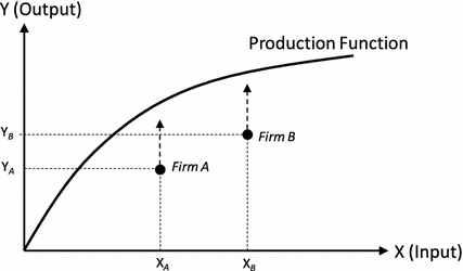
Economic efficiency and production frontier
Fig. 2 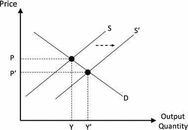
Change in supply and equilibrium price
This is consistent with an output-oriented efficiency analysis in the productivity literature [15].
This is consistent with a profit maximization model, given fixed input prices and levels.
The output level \(\bar{y}_r\) will be chosen by all firms. Clearly, the firms using input levels less than \(X_r\) will only be able to produce the output level defined by the production frontier. And firms using more than \(X_\mathrm{r}\) input cannot adjust their input levels by assumption, so they will produce \(\bar{y}_r\) with more than \(X_\mathrm{r}\) input.
Note that all output variables need to be normalized in data pre-processing to eliminate unit dependence.
For a discussion of the relationship among these properties see the weak, moderate, and strong dominance section in the on-line electronic supplementary material.
Note the exchange of \(q\) and \(h\).
This result is illustrated in Table 2, Case 2, DC 5.
In a special case, in which input markets are perfectly competitive \(\beta _{jl} =0\), the inverse supply function will be constant and the cost function becomes a linear function. This does not affect the optimality condition, i.e., the profit function is still a strictly concave function if the revenue function is strictly concave.
Weakly efficient frontier is defined as the portion of the input (output) isoquant along which one of the inputs (outputs) can be reduced (expanded) while holding all other netputs constant and remaining on the isoquant; see Färe and Lovell [34] for more details.
Bougnol and Dulá [35] propose a procedure to identify anchor points and show that, if a point is an anchor point, then increasing an input or decreasing an output generates a new point on the free-disposability portion of the production possibility set.


References
Cherchyea, L., Kuosmanen, T., Post, T.: Non-parametric production analysis in non-competitive environments. Int. J. Prod. Econ. 80, 279–294 (2002)
Fried, H.O., Lovell, C.A.K., Schmidt, S.S.: The Measurement of Productive Efficiency and Productivity Growth. Oxford University Press, Oxford (2008)
Farrell, M.J.: The measurement of productive efficiency. J. R. Stat. Soc., Ser. A, Gen. 120, 253–281 (1957)
Leibenstein, H.: Allocative efficiency versus ’X-efficiency’. Am. Econ. Rev. 56, 392–415 (1966)
Leibenstein, H., Maital, S.: The organizational foundation of X-inefficiency: a game theoretic interpretation of Argyris’ model of organizational learning. J. Econ. Behav. Organ. 23, 251–268 (1994)
Stigler, G.: The Xistence of X-efficiency. Am. Econ. Rev. 66, 213–216 (1976)
Foster, L., Haltiwanger, J., Syverson, C.: Reallocation, firm turnover, and efficiency: selection on productivity or profitability? Am. Econ. Rev. 98(1), 394–425 (2008)
Bloom, N., van Reenen, J.: Measuring and explaining management practices across firms and countries. Q. J. Econ. 122(4), 1351–1408 (2007)
Bogetoft, P., Hougaard, J.L.: Rational inefficiencies. J. Prod. Anal. 20, 243–271 (2003)
Cournot, A.A.: Recherches sur les Principes Mathématiques de la Théorie des Richesses. Librairie des sciences politiques et sociales, M. Rivière et cie, Paris (1838)
Nash, J.F.: Equilibrium points in n-person games. Proc. Natl. Acad. Sci. 36, 48–49 (1950)
Nash, J.F.: Noncooperative games. Ann. Math. 45, 286–295 (1951)
Rosen, J.B.: Existence and uniqueness of equilibrium points for concave n-person games. Econometrica 33(3), 520–534 (1965)
Arrow, K.J., Debreu, G.: Existence of an equilibrium for a competitive economy. Econometrica 22(3), 265–290 (1954)
Färe, R., Primont, D.: Multi-Output Production and Duality: Theory and Applications. Kluwer Academic Publishers, Boston (1995)
Murphy, F.H., Sherali, H.D., Soyster, A.L.: A mathematical programming approach for determining oligopolistic market equilibrium. Math. Program. 24, 92–106 (1982)
Harker, P.T.: A variational inequality approach for the determination of oligopolistic market equilibrium. Math. Program. 30, 105–111 (1984)
Bonanno, G.: General equilibrium theory with imperfect competition. J. Econ. Surv. 4(4), 297–328 (1990)
Boles, J.N.: Efficiency squared-efficient computation of efficiency indexes. In Western Farm Economic Association, Proceedings 1966, Pullman, Washington, pp. 137–142 (1967)
Afriat, S.N.: Efficiency estimation of production functions. Int. Econ. Rev. 13(3), 568–598 (1972)
Charnes, A., Cooper, W.W., Rhodes, E.: Measuring the efficiency of decision making units. Eur. J. Oper. Res. 2, 429–444 (1978)
Lee, C.-Y., Johnson, A.L.: Proactive data envelopment analysis: effective production and capacity expansion in stochastic environments. Eur. J. Oper. Res. 232(3), 537–548 (2014)
Facchinei, F., Pang, J.S.: Finite-dimensional Variational Inequalities and Complementarity Problems. Springer, New York (2003)
Gabay, D. Moulin, H.: On the uniqueness and stability of Nash-equilibria in noncooperative games. In Applied Stochastic Control in Economics and Management Science, A. Bensoussan, P. Kleindorfer, C. S. Tapiero, editors, North-Holland, Amsterdam, The Netherlands, pp. 271–294 (1980)
Karamardian, S.: Generalized complementarity problem. J. Optim. Theory Appl. 8, 161–168 (1971)
Dyson, G., Thanassoulis, E., Boussofiane, A.: Data envelopment analysis. In: Hendry, L.C., Eglese, R.W. (eds.) Tutorial Papers in Operational Research. Operational Research Society, Birmingham (1990)
Farahat, A., Perakis, G.: A nonnegative extension of the affine demand function and equilibrium analysis for multiproduct price competition. Oper. Res. Lett. 38, 280–286 (2010)
Bernstein, F., Federgruen, A.: Comparative statics, strategic complements and substitutes in oligopolies. J. Math. Econ. 40, 713–746 (2004)
Shubik, M., Levitan, R.: Market Structure and Behavior. Harvard University Press, Cambridge (1980)
Soon, W.M., Zhao, G.Y., Zhang, J.P.: Complementarity demand functions and pricing models for multi-product markets. Eur. J. Appl. Math. 20(5), 399–430 (2009)
Marshall, A.: Principles of Economics, 8th edn. Macmillan and Co., Ltd., London (1920)
Stigler, G.: Production and distribution in the short run. J. Political Econ. 47(3), 305–327 (1939)
Färe, R., Grosskopf, S., Lovell, C.A.K.: Production Frontiers. Cambridge University Press, New York (1994)
Färe, R., Lovell, C.A.K.: Measuring the technical efficiency of production. J. Econ. Theory 19, 150–162 (1978)
Bougnol, M.-L., Dulá, J.H.: Anchor points in DEA. Eur. J. Oper. Res. 192(2), 668–676 (2009)
Acknowledgments
The authors thank Steven Puller and Robin C. Sickles for providing constructive suggestions and helpful discussion. Any errors are the responsibilities of the authors. This research was partially funded by National Science Council, Taiwan (NSC101-2218-E-006-023), and Research Center for Energy Technology and Strategy at National Cheng Kung University, Taiwan.
Author information
Authors and Affiliations
Corresponding author
Additional information
Communicated by Kaoru Tone.
Electronic supplementary material
Below is the link to the electronic supplementary material.
Rights and permissions
About this article
Cite this article
Lee, C.Y., Johnson, A.L. Measuring Efficiency in Imperfectly Competitive Markets: An Example of Rational Inefficiency. J Optim Theory Appl 164, 702–722 (2015). https://doi.org/10.1007/s10957-014-0557-z
Received:
Accepted:
Published:
Issue Date:
DOI: https://doi.org/10.1007/s10957-014-0557-z