Statistical Physics Analysis of Maximum a Posteriori Estimation for Multi-channel Hidden Markov Models

Abstract

The performance of Maximum a posteriori (MAP) estimation is studied analytically for binary symmetric multi-channel Hidden Markov processes. We reduce the estimation problem to a 1D Ising spin model and define order parameters that correspond to different characteristics of the MAP-estimated sequence. The solution to the MAP estimation problem has different operational regimes separated by first order phase transitions. The transition points for L-channel system with identical noise levels, are uniquely determined by L being odd or even, irrespective of the actual number of channels. We demonstrate that for lower noise intensities, the number of solutions is uniquely determined for odd L, whereas for even L there are exponentially many solutions. We also develop a semi analytical approach to calculate the estimation error without resorting to brute force simulations. Finally, we examine the tradeoff between a system with single low-noise channel and one with multiple noisy channels.

1 Introduction

In many dynamical systems direct observation of the internal system state is not possible. Instead, one has noisy observations of those states. When the internal dynamics is governed by a Markovian process, the resulting systems are known as Hidden Markov Models, or HMMs. HMM is the simplest tool to model the systems where a correlated data passes through a noisy channel [1, 2]. It is used extensively to model such physical systems and finds applications in various areas such as signal processing, speech recognition, bioinformatics and so on [3, 4].

One of the major problems underlying HMMs is the estimation of the hidden state sequence given the observations, which is usually done through maximum a posteriori (MAP) estimation technique. A natural characteristic of MAP estimation is the accuracy of estimation, i.e., the closeness of the original and estimated sequence. Another important characteristic is the number of solutions it produces in response to a given observed sequence. This is related to the concept of trackability, which describes whether the number of hidden state sequences grows polynomially (trackable) or exponentially (non-trackable) with the length of the observed sequence. For so called weak models,¹ it was established that there is a sharp transition between trackable and non-trackable regimes as one varies the noise [5]. A generalization to the probabilistic case was done for a binary symmetric HMM [6], where it was shown that the non-trackability is related to finite zero-temperature entropy of an appropriately defined Ising model. In particular, [6] demonstrated that there is a critical noise intensity above which the number of MAP solutions is exponential in the length of the observed sequence.

In this work we study the performance of MAP estimation for the scenario where the hidden dynamics is observed via multiple observation channels, which we refer to as multi-channel HMMs. Multi channel HMM is a more robust way of modeling multi channel signals, such as in sensor networks where local readings from different sensors are used to make inference about the underlying process. Note that the channels can generally have different characteristics, i.e., measurement noise. Here we assume that the readings of the channels are conditionally independent given the underlying hidden state.

One of our main results is that the presence of additional observation channels does not always improve the inference in the sense of above characteristics. In particular, in systems with even number of channels and identical noise intensities, there is always an exponential number of solutions for any noise intensity, indicated by a finite zero-temperature entropy of the corresponding statistical physics systems. Intuitively, this happens because of conflicting observations from different channels, which produces a macroscopic frustration of spins in the system. Furthermore, for two-channel systems with generally different noise characteristics, we calculate the phase boundary between the regions of zero and non-zero entropy regimes in the parameter space. In all the systems studied with single or multiple channels, we observe discontinuous phase transitions in the thermodynamic quantities with the variation of noise. The points of phase transitions are the same for all the even number channel systems. This is also true for any of the odd number channel systems but the transition points are different from that of the even number channel systems.

For general L-channel systems with identical noise in the channels, we calculate the different statistical characteristics of MAP for this scenario, and find that the average error between the true and estimated sequences reduces with the addition of channels. Furthermore, we bring in the notion of channel cost which lets us explore the tradeoff between the total cost and error that one can tolerate in the system. Finally, we also analyze the performance of MAP estimation for Gaussian noise, and find that the entropy is always zero, so that one has exactly one solution for every observed sequence. This suggests that the existence of exponentially degenerate solution relates to the discreteness.

Let us provide a brief outline of the structure of our paper: We start by providing some general information about Maximum a Posteriori estimation in Sect. 2. We introduce binary symmetric HMMs and describe the mapping to an Ising model in Sect. 3. In Sect. 3.3 we describe the statistical physics approach to MAP estimation for multi-channel binary HMMs and define appropriate order parameters for characterizing MAP performance. Section 4 describes the solution of the model. The recurrent states are given in Sect. 5 followed by presentation of results in Sect. 6. Section 6.1 focuses on a detailed analysis for two observation channel scenario and Sect. 6.2 provides results for the multiple channel scenario. In Sect. 6.3 we discuss about the cost of designing a multiple channel system and its impact on the system performance relative to a single channel system. Finally, we conclude by discussing our results and future work. In the Appendix, we give details about analytical calculation of MAP accuracy and elaborate on the Gaussian observation model along with the main differences from the binary symmetric case.

2 MAP Estimation

The present work focuses on a specific class of stochastic processes, namely, the binary symmetric HMMs although the techniques of MAP estimation can be applied to general stochastic processes too. In this section, we give a brief idea on MAP estimation for generalized HMMs and defer to the study of binary symmetric HMMs in Sect. 3.

Let us consider x=(x ₁,…,x _N ) as the signal generating sequence. The observation in L different channels at every time instant can be generically written as $\underline{\mathbf {y}} = (\mathbf {y}^{1},\ldots,\mathbf {y}^{L})$ with $\mathbf {y}^{i}=(y_{1}^{i},\ldots,y_{N}^{i}) |_{\{ i=1,\ldots,L\}}$. Here x and $\underline{\mathbf {y}}$ are the realizations of discrete time random processes and ; with i being the index for the observation channel as shown in Fig. 1. y ⁱ’s are the noisy observations of obtained from different observation channels. The observations from different channels are mutually conditionally independent given the signal x and are described by the conditional probability p(y ⁱ|x). The observed sequences y ⁱ’s are considered to be given along with the probabilities p(y ⁱ|x) and p(x). Thus, we are required to find the generating sequence x from the given sets of observation sequences.

Fig. 1

Hidden Markov model with multiple observation sequences (Color figure online)

MAP provides a method to estimate the generating sequence ${\hat{\mathbf {x}}}$ on the basis of the observations y ⁱ. ${\hat{\mathbf {x}}}$ is found by maximizing over x the posterior probability,

Since p(y ¹,…,y ^L) does not depend on x, we can equivalently minimize the Hamiltonian which is given by,

(1)

where by log we imply natural logarithm. Because of the mutual independence between the observations conditioned on x, we can rewrite $H(\underline{\mathbf {y}},\mathbf {x})$ as

(2)

The advantage of using $H(\underline{\mathbf {y}},\mathbf {x})$ is that, if is ergodic² (which we will assume in the rest of the paper), then for N≫1, $H(\underline{\mathbf {y}},\hat{\mathbf {x}}(\underline{\mathbf {y}}))$ will be independent from $\underline{\mathbf {y}}$, , being the typical set of  [7]. The typical set is the set of sequences whose sample entropy is close to the true entropy, where entropy is a measure of uncertainty of a random variable and is a function of the probability distribution of the sequences in . The typical set has total probability close to one, a consequence of the asymptotic equipartition property (AEP) [7]. Thus for N≫1, the sequence (y ¹,…,y ^L) will lie in the typical set of with high probability. As a result, we have and all elements of have equal probability. We can take advantage of this and use for $H(\underline{\mathbf {y}},\hat{\mathbf {x}}(\underline{\mathbf {y}}))$ the averaged quantity $\sum _{\underline{\mathbf {y}}} \mathbf{p}(\underline{\mathbf {y}})H(\underline {\mathbf {y}},\hat{\mathbf {x}}(\underline{\mathbf {y}}))$.

Let us consider some extreme cases of noise in the observation channels. Since we are dealing with more than one observation channel we have to consider the overall contribution from different channels with varying noise. When we refer to the weak and strong noise in the channels we will be referring with respect to the noisiest channel of the whole set. The other channels will be relatively cleaner and modify the overall performance. For the case (i) when the noise applied to the channels is very weak, $\mathbf{p}(\mathbf {x}|\underline{\mathbf {y}}) \cong \prod_{i=1}^{L} \prod_{k=1}^{N} \delta(x_{k} - y_{k}^{i})$. This results in recovering the generating sequence almost exactly and (ii) for the case of strong noise in channels the estimation is prior dominated, i.e. $\mathbf{p}(\mathbf {x}|\underline{\mathbf {y}}) \cong\mathbf{p}(\mathbf {x})$, and hence is not informative. Without any prior imposed, p(x)∝const. Here, the MAP estimation reduces to the maximum likelihood (ML) estimation scheme. It should be noted that using ML estimate we can also obtain the exact sequence in the low noise regime.

Minimization of Hamiltonian from (1) for a given $\underline{\mathbf {y}}$ can be readily done using the Viterbi algorithm, but it produces one single optimal estimate $\hat{\mathbf {x}}(\underline{\mathbf {y}})$. For completeness we should also seek for other possible sequences $\hat{\mathbf {x}}^{[\gamma]}(\underline{\mathbf {y}})$ for which $H(\underline{\mathbf {y}},\hat{\mathbf {x}}^{[\gamma]}(\underline{\mathbf {y}}))$ (greater than $H(\underline{\mathbf {y}},\hat{\mathbf {x}}(\underline{\mathbf {y}}))$) is almost equal to the optimal estimated Hamiltonian in large N limit. Under that approximation we have

$$\lim_{N \rightarrow\infty} \frac{H(\underline{\mathbf {y}},\hat{\mathbf {x}}^{[\gamma]}(\underline{\mathbf {y}}))}{N}=\lim_{N \rightarrow\infty} \frac{H(\underline{\mathbf {y}},\hat{\mathbf {x}}(\underline{\mathbf {y}}))}{N}. $$

These obtained sequences from the MAP estimate are equivalent for N→∞ and can be listed as,

(3)

with denoting the number of such possible sequences. If , the ergodicity argument can be used to obtain the logarithm of the number of solutions for the observed typical sequence,

(4)

In the limit N→∞, a finite value of $\theta=\frac {\varTheta}{N}$ implies that there are exponentially many outcomes of minimizing $H(\underline{\mathbf {y}},\mathbf {x})$ over x. The term Θ is called entropy from analogy with the Ising spin model as will be explained in detail in the subsequent sections.

Various moments of $\hat{\mathbf {x}}^{[\gamma]}(\underline{\mathbf {y}})$ are calculated, which are random variables due to the dependence on $\underline{\mathbf {y}}$. The knowledge of the moments along with the error analysis is employed to characterize the accuracy of the estimation. For weak noise these moments are close to the original process . We also evaluate the average overlap between estimated sequences $\hat{\mathbf {x}}^{[\gamma]}(\underline{\mathbf {y}})$ and the observed sequences $\underline{\mathbf {y}}$. If the overlap is close to one, it would imply a observation dominated estimation of the sequence.

3 Binary Symmetric Hidden Markov Processes

3.1 Definition

We analyze a binary, discrete-time Markov stochastic process . Each random variable x _k can have only two realizations x _k =±1. The Markov feature implies,

(5)

where p(x _k |x _k−1) is the time-independent transition probability of the Markov process. The state diagram for the binary, discrete time Markov process is shown in Fig. 2. We parameterize the binary symmetric situation by a single number 0<q<1, with p(1|1)=p(−1|−1)=1−q and p(1|−1)=p(−1|1)=q and the stationary state distribution is considered to be uniform $p_{\mathrm{st}}(1)=p_{\mathrm{st}}(-1)=\frac{1}{2}$. The noise process is assumed to be memory-less, time independent and unbiased. Thus,

(6)

where $\pi^{i}(y_{k}^{i}|x_{k})$ is the probability of observing y _k in channel i given the state x _k . For the ith channel π ⁱ(−1|1)=π ⁱ(1|−1)=ε _i ,π ⁱ(1|1)=π ⁱ(−1|−1)=1−ε _i ; ε _i being the probability of error in the ith channel. Here memory-less refers to the factorization in (6), time independence refers to the fact that π ⁱ(…|…) does not depend on k, and finally unbiased means that the noise acts symmetrically on both realizations of the Markov process, i.e., π ⁱ(1|–1)=π ⁱ(–1|1). Starting from this, we vary the noise between multiple observation channels and study its effect in the sequence decoding process. In Appendix 8.2 we discuss a more general case involving Gaussian distribution of noise realizations in the observation channels. The detailed formalism is done for the case of a single observation channel.

Fig. 2

State diagram for a binary symmetric Markov chain (Color figure online)

The composite process with realizations $(y_{k}^{i},x_{k})$ is Markov even though in general is not a Markov process. The transition probabilities for the ith observation channel can be written as,

(7)

3.2 Mapping to the Ising Model

The problem can be efficiently mapped to the Ising spin model where we will represent the transition probabilities as,

(8)

The observation probabilities for binary symmetric noise are given as,

(9)

and that for the Gaussian distribution of noise in the observation channels is given by,

(10)

where $\sigma_{i}^{2}$ is the noise variance.

Combining (9) with (1) and with the help of (5) and (6) we represent the log-likelihood for the case with binary symmetric noise realization as,

(11)

The same for the Gaussian distribution of noise (see (10)) is given as,

(12)

which simply reduces to,

(13)

The redundant additive factors are omitted from final expressions of the Hamiltonian. The subscripts ‘B’ and ‘G’ denote the binary and Gaussian cases respectively. $H(\underline{\mathbf {y}},\mathbf {x})$ (representing the general Hamiltonian for both ‘B’ and ‘G’) is the Hamiltonian of a (1d) Ising model with external random fields governed by the probability $\mathbf{p}(\underline{\mathbf {y}}|\mathbf {x})$ [8]. The factor J is the spin-spin interaction constant, uniquely determined by the transition probability q. For $q<\frac{1}{2}$, the constant J is positive. This refers to the ferromagnetic situation where the spins tend to align in the same direction. The random-fields (within the Ising model) obtained in the expression for $H(\underline{\mathbf {y}},\mathbf {x})$ display a non-Markovian correlation. This is different from what is known for the random fields from the literature, that are in general uncorrelated [9, 10]. For all calculations, we assume J,h _i ,σ _i >0. Let us also introduce another parameter α=h ₂/h ₁ which represents the ratio of the noise between two observation channels (subscripts 1 and 2 refer to the two observation channels) and is assumed to be a positive integer.

3.3 Statistical Physics of MAP Estimation

We now implement the MAP estimation to minimize the Hamiltonian $H(\underline{\mathbf {y}},\mathbf {x})$. In Sect. 2 we argued that this is equivalent to minimizing $\sum _{\underline{\mathbf {y}}} \mathbf{p}(\underline{\mathbf {y}})H(\underline{\mathbf {y}},\hat{\mathbf {x}}(\underline{\mathbf {y}}))$. For this purpose let us introduce a non-zero temperature $T=\frac {1}{\beta} \geq 0$ and write the conditional probability as,

(14)

where $Z(\underline{\mathbf {y}})$ is the partition function. Using ideas from statistical physics, we find that $\rho(\mathbf {x}|\underline{\mathbf {y}})$ gives the probability distribution of states x for a system with Hamiltonian $H(\underline{\mathbf {y}},\mathbf {x})$. The system is assumed to be interacting with a thermal bath at temperature T, and with frozen random fields $h_{i} y^{i}_{k}$ [11]. For T→0, and a given $\underline{\mathbf {y}}$, the individual terms of the partition function are strongly picked at those $\hat{\mathbf {x}}(\underline{\mathbf {y}})$ which minimize the Hamiltonian $H(\underline{\mathbf {y}},\mathbf {x})$ to get to the ground states. If, however, the limit T→0 is applied after the limit N→∞ we get,

(15)

where $\hat{\mathbf {x}}^{[\gamma]}(\underline{\mathbf {y}})$ and are given by (3). We are going to work on this low temperature regime from now on.

The average of $H(\underline{\mathbf {y}},\mathbf {x})$ in the T→0 regime will equal its value minimized over x,

(16)

where by assumption all ground state configurations $\hat{\mathbf {x}}(\underline{\mathbf {y}})$ have the same energy $H(\underline{\mathbf {y}},\hat{\mathbf {x}}^{[\gamma]}(\underline{\mathbf {y}}))=H(\underline {\mathbf {y}},\hat{\mathbf {x}}^{[1]}(\underline{\mathbf {y}}))$ for any γ.

The zero-temperature entropy Θ depicting the number of MAP solutions and is given as,

(17)

Another important statistical parameter, free energy can also be defined as,

(18)

where the Ising Hamiltonian $H(\underline{\mathbf {y}},\mathbf {x})$ is given by (11) or (13). With the help of this definition we can now define the entropy Θ in terms of the free energy as,

(19)

We also define the order parameters which are the relevant characteristics of MAP below,

(20)

(21)

c accounts for the correlation between the neighboring spins in the estimated sequence and v measures the overlap between the estimated and the observed sequences for the various cases that are studied.

The order parameters defined above are indirect measures of estimation accuracy. Calculation of direct error involves evaluating the overlap between the actual hidden sequence that generates a given observation sequence, and the inferred sequence based on the observation sequence. Since we are interested in average quantities, it is clear that calculating the average error amounts to finding the overlap between a typical hidden sequence and its MAP estimate, i.e.,

(22)

where $\mathbf{s} = \{s_{k}\}_{k=1}^{N}$ is a typical sequence generated by the (hidden) Markov chain. Let us define a modified Hamiltonian,

(23)

Further, let us introduce f _g which is related to the free energy F _g of the modified Hamiltonian by $f_{g}=\frac{F_{g}}{N}$. It is given by,

(24)

With this the overlap can be simply given by Δ=−∂ _g f _g | _{g→0,β→∞}, where the limits are taken in the order g→0,β→∞.

4 Solution of the Model

Here we will solve for the order parameters and entropy of multiple observation channels using tools that we developed using the Ising spin model. The solution of the model for L=1 was provided in [6]. To make the paper self-contained, here we repeat the main steps of the derivation. Let us recall the partition function (14) which for L observation sequences can be written as,

(25)

Summing over the first spin yields the following transformation for $Z(\underline{\mathbf {y}})$,

(26)

where $\xi_{2}=A(\xi_{1}) + \sum ^{L}_{i=1}h_{i} y^{i}_{2}$, $\xi_{1}=\sum ^{L}_{i=1}h_{i} y^{i}_{1}$ and,

(27)

(28)

Hence, once the first spin is excluded from the chain the field acting on the second spin changes from $\sum ^{L}_{i=1}h_{i} y^{i}_{2}$ to $\sum ^{L}_{i=1}h_{i} y^{i}_{2}+A(\xi_{1})$. In the zero temperature limit (T→0 ; β→∞) the functions A(u) and B(u) reduce to the following form,

(29)

(30)

where ϑ(x)=0 for (x<0) and ϑ(x)=1 for (x>0). Thus after excluding one spin every time and repeating the above steps, the partition function for the system is obtained as,

(31)

where ξ _k is obtained from the recursion relation

(32)

Following similar steps with H _G from (13) we get the recursion relation for the Gaussian realization of noise in the observation channel as,

(33)

$y^{i}_{k}$’s from the above random recursion relation are random quantities governed by the probability $\mathbf{p}(\underline{\mathbf {y}})$. As we can see from the above equations for binary realizations, $y^{i}_{k}$ can take a finite number of values and ξ _k can take an infinite number of values. But in the asymptotic β→∞ limit, A(u) and B(u) reduce to the simple form given in (29) and (30) respectively. Thus we obtain a finite number of values for ξ _k (the number can be large or small). However for the Gaussian distribution, we get a continuous set of values for ξ _k .

The parametric form of ξ _k is already explained in [6] for a single observation channel. Here we provide the generalization to two observation channels, i.e. L=2, which can be easily extended to the multiple channel case. We can parameterize ξ _k as, ξ _k (n ₁,n ₂,n ₃)=(n ₁ h ₁+n ₂ h ₂+n ₃ J)=([n ₁+αn ₂]h ₁+n ₃ J), where h ₂/h ₁=α, n ₁ and n ₂ can be positive and negative integers while n ₃ can take only three values 0,±1. It may be noted that the states ξ(n ₁,n ₂,0) are not recurrent: once ξ _k takes a value with [(n ₁+αn ₂) positive or negative, n ₃=±1] it never comes back to the state ξ(n ₁,n ₂,0). Thus in the limit N≫1 we can ignore the states ξ(n ₁,n ₂,0).

Let us now consider the problem of finding the stationary distribution of the random process given by (32). Note that the process with probabilities $\mathbf{p}(\underline{\mathbf {y}})$ is not Markovian, hence the process in (32) is not Markovian either, which slightly complicates the calculation of its stationary distribution. Towards the latter goal, let us consider an auxiliary Markov process , which has identical statistical characteristics with the process . For this auxiliary Markov process the realization is denoted as z, so as not to mix with the original process x. We need to include to make the composite process Markov. Thus, to make the realizations for the composite process [ξ,y ¹,…,y ^L] Markov, we enlarge it to [ξ,y ¹,…,y ^L,z] (lets call it ). 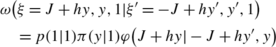The conditional probability for is given by,

(34)

For , p(z|z′) and π(y ⁱ|z) refer to the Markov process and the noise respectively, while φ(ξ|ξ′,y ¹,…,y ^L) takes only two values 0 and 1, depending on whether the transition is allowed by the recursion (32). Now, we need to determine φ(ξ|ξ′,y ¹,…,y ^L) after finding all possible values of ξ _k . Let us first relate the stationary probabilities ω(ξ,y ¹,…,y ^L,z) of the composite Markov process to the characteristics of MAP estimation: ω(ξ,y ¹,…,y ^L,z), conveys the message about the stationary probabilities ω(ξ). After this using the definition for the partition function from (31) and free energy (18) for the composite Markov process which is ergodic, the free energy is given as [9],

$$ \everymath{\displaystyle }\begin{array}{lll} -f(J,h)\equiv-F(J,h)/N=\sum _{\xi} \omega(\xi) B(\xi); \cr\noalign{\vspace{3pt}} \omega(\xi)=\sum _{y^1,\ldots,y^L,z} \omega \bigl(\xi ,y^1, \ldots,y^L,z \bigr) \end{array}$$

(35)

where the summation is taken over all possible values of ξ [for a given (J,h)]. We study different processes in the multi-channel scenario, generally speaking, for L>2 with same noise in the channels and for L=2 with varying noise in the two channels. For all these cases h _i ’s can be represented by a single quantity h. Once we find f(J,h) we can apply (20), (21) to do further calculations. To calculate the entropy we first derive a convenient expression for free energy, which can be obtained from (30), (31).

(36)

Using this we find,

(37)

where δ(.) is the Kronecker delta function and δ(ξ _k ±J)=δ(ξ _k +J)+δ(ξ _k −J). In the N≫1 limit, under the assumption that the Markov process is ergodic, $\frac{1}{N}\sum _{k=1}^{N} \delta(\xi_{k} \pm J )$ should with probability one (for the elements of the typical set ) converge to ω(ξ=J)+ω(ξ=−J). We thus obtain [9],

(38)

The above formula for an Ising spin model would imply that the zero temperature entropy can be extensive only when the external field ξ acting on the spins would have the same energy ξx _k =±1 as the spin-spin coupling constant J. This would imply that a macroscopic amount of spin (from any of the models studied) is frustrated, i.e., the factors influencing those spins compensate each other. When the entropy is not zero, there are many sequences whose probability may still slightly differ from one another. The MAP characteristics (c,v) would refer to the averages over all those equivalent sequences. We will discuss this effect explicitly for the various cases analyzed. For the sake of completeness, we provide here the analytical expressions for the order parameters c and v obtained by using (36) in (20) and (21).

(39)

(40)

Finally, we discuss the semi-analytical error analysis that has been developed in this work. For this let us consider the overlap defined in (22). Recall that the error estimate is given by −∂ _g f _g | _{g→0,β→∞} where f _g is defined in (24). Derivation is shown explicitly for a single observation channel in Appendix 8.1. The results are used to analytically solve for the error in single and two observation channels and is provided in Sect. 6.1. The formalism can easily be generalized for multiple observation channels with some tedious algebra. In Appendix 8.1 we show that the overlap between the estimated sequence x and true sequence s is given as,

(41)

In the limit N→∞, Δ _k is independent of k. The average error is related to the overlap Δ _k as, $P_{\mathit{MAP}} \{ \mathit{error}\}=\frac{1-\Delta}{2}$.

5 Characterization of the Recurrent States

For calculating the quantities of interest we need to obtain the recurrent states for the different multi-channel systems. The recurrent states are found out and parameterized in a manner similar to that demonstrated for L=1 in [6]. In this section we analyze two scenarios. In Scenario I, we consider a 2 observation channel system. The noise in either channel is varied in a certain fixed proportion. In Scenario II, we consider the general L>2 channel system, each having the same noise intensity. Below we give the parameterizations of the recurrent states for these two cases separately. In both the scenarios we come across multiple phase transitions which we denote by m and the noise within any of those phases varies as $\frac{2J}{m}<h<\frac{2J}{m-1}$. The phase transitions are reflected in the study of the order parameters and the error analysis and is discussed in detail in the next section.

5.1 Scenario I: Two Channels with Different Noise Intensities

The parameter α=h ₂/h ₁ is defined as the ratio between h _i ’s (9) in the individual observation channels. The stationary states can be parameterized as, $[a_{i} \ \ \bar{a}_{i}]$ which are written in terms of h (depicting the channel with higher noise),

$$ \everymath{\displaystyle }\begin{array}{lll} a_i=J+(2-i)h+ \eta h \cr\noalign{\vspace{3pt}} \bar{a}_i=-J-(2-i)h+ \eta h \end{array}$$

(42)

The quantity η is defined as,

(43)

The values of α=h ₂/h ₁ are kept as positive integers since for an arbitrary α (rational or irrational) the number of stationary states increases very fast making the analysis complicated, but doesn’t contribute towards any additional generality of the problem. The stationary states at all the phases can be found form the above formula by substituting the values of i from Table 1 in the above equation. The total number of states during different phases is tabulated in Table 2.

Table 1 The possible values of i for different α at different phases denoted by m. In the table below (…) implies for (i) α:even, all integer values on the range and (ii) α:odd, only the even values in the range

Table 2 Number of states for different α at different phases denoted by m

5.2 Scenario II: L-Identical Channels

For a multiple observation channel system we can parameterize the stationary states for a given value of J and h within any phase as,

$$ \everymath{\displaystyle }\begin{array}{lll} b_i=J+(2-i)h+ \sum _{i=1}^L t_i h \cr\noalign{\vspace{3pt}} \bar{b}_i=-J-(2-i)h+ \sum _{i=1}^L t_i h \end{array} $$

(44)

with t _i ∈{+1,−1}. The possible values of i for different phases are given in Table 3. For the various possible phases, the total number of states are given in Table 4. Here one can notice the significant rise in the total number of states for large L as we go to a higher phase.

Table 3 The possible values of i for multiple observation channel systems with same h at different phases denoted by m. In the table below (…) implies for (i) $L:\emph{odd}$, all integer values on the range and (ii) $L:\emph{even}$, only the even values in the range

Table 4 Number of states for multi observation channels with same h at different phases denoted by m

6 Results

In this section we describe our results where we try to analyze different multiple observation channel systems by evaluating the order parameters and entropy. First, we consider a 2 observation channel system by varying the noise in the individual channels. Next, we consider L observation channels with identical noise intensities. Finally, we compare the performance of a single relatively “clean” channel with multiple “noisy” ones by bringing in the notion of channel cost, and examine the tradeoffs between the two setups. An attempt is made to provide a physical intuition behind the results that we obtained using simple thermodynamic principles [9, 12–15]. The system performance is considered for both maximum likelihood (ML) as well as maximum a posteriori (MAP) estimation. In ML, the estimation of the current state is dependent only on the observations from the different channels at that particular instant. In case of a tie, which arises when the number of observation channels is even, the state is chosen randomly to be either 0 or 1 with equal probability. For example, suppose the number of observation channels is L (L being even) with L/2 of the channels having an observation 1 and the remaining L/2 an observation of 0. In this case, the state is chosen to be either 0 or 1 at random with probability 1/2.

6.1 Two-Channel Scenario

In this subsection, we study the performance of a two observation channel system with relatively different noise levels.

Channel 1 has noise ε ₁ and channel 2 has noise ε ₂. The parameter α defines the relation between the noise levels in the two channels. Specifically,

Since we always take α≥1,³ the noise level in channel 2 is less than that in channel 1, implying channel 1 is “noisier” than channel 2. The order parameters c and v, plotted by varying the noise ε ₁ ⁴ in channel 1 for a fixed spin-spin correlation J (a function of q as given by (8)), are shown in Fig. 3. We observe different operational regimes, that are separated by first order phase transitions. The point of the first phase transition gradually moves to the right with an increase in α. This indicates that the overall behavior is dominated by that of the cleaner channel, which is intuitive. In this region before the first phase transition, the ML and MAP estimates coincide. The sequence correlation parameter c is pretty stable and noise independent before the point of first phase transition for MAP estimation. Afterwards the correlation shows discrete jumps and goes to the prior dominated value of 1 as observed from MAP estimation, whereas with the ML estimate, c monotonically reduces to 0. The advantage of MAP estimation over ML is the fact that in MAP the estimation is supported by prior and hence, performs better at intermediate noise ranges. For example, when α=2, it can be seen that the correlation c degrades faster for ML estimation and is nearly constant for a large range of noise values for MAP estimation. The overlap v is found to gradually shift towards 1 before the first phase transition with increase in the value of α, implying that the estimated sequence for all the possible noises is primarily driven by the observations. Before first phase transition, we encounter the observation dominated regime except for α=1. The value of the overlap is not 1 because of the manner the overlap is defined in (21). A more plausible way to see the observation dominated regime is to consider the overlap between MAP and ML estimated sequences, which is plotted in Fig. 3(c). This confirms the fact that there is no observation dominated regime for α=1 in 2-channel systems. After the first phase transition the overlap becomes worse and at higher noise, v decays towards 0. Increasing α enlarges the observation dominated regime, or in other words, the region of ML estimation. It is also interesting to note that the correlation and overlap parameter are stable for a longer range with an increase in α, but show a rapid rise or decay respectively after the first phase transition. The analytical results are verified by simulations using Viterbi algorithm⁵ which are in good agreement with each other.

Fig. 3

Order parameters (a) c and (b) v obtained analytically by Ising Hamiltonian minimization (bold line) which shows an exact superposition with the data obtained from the Viterbi algorithm (open squares) for two channels with different noise for q=0.24. The smooth decaying lines in the plot for c are obtained via ML estimate and the horizontal blue line depicts c ₀. (c) v ₁ is the overlap between the MAP and ML estimated sequences (Color figure online)

Let us now focus on entropy. We see that the addition of a second observation channel with the same noise as the first results in non-zero entropy for all possible values of ε. With the introduction of the second observation channel, the noise parameter h ₂ being of same strength as h ₁ mutually cancel each other. This gives rise to multiple degenerate ground states for the acting external field and hence multiple solutions are obtained from MAP estimation, resulting in non-zero entropy [9]. However as we increase α, it can be seen from Fig. 4 that the regions of zero entropy is obtained again and the point of first phase transition shifts to the right. However, after the first phase transition, the entropy rises, attains a maxima and then decays. The reason behind this is discussed in detail below where we discuss the regions of zero and non-zero entropies obtained for parameter q.

Fig. 4

The entropy of the system obtained analytically with varying ε (ε denoting the higher noise level) for two observation channels at different noise ratios given by α at q=0.24 (Color figure online)

Knowing the region of zero and non-zero entropy is of particular interest for the two observation channel system. We derive this region for the possible values of noise, ε in the two observation channels for parameter q and this is plotted in Fig. 5. We can qualitatively see that for the region corresponding to ε ₁=ε ₂ line which defines α=1, we can never obtain a unique sequence from MAP estimation. This is due to the prevalence of degenerate ground state solutions obtained at zero temperature due to the mutual nullification of the opposing field in the two observation channels. As we perturb the external random field applied in one of the observation channels by a certain amount (depending on the value of q), we migrate to the region of zero entropy. The region above the ε ₁=ε ₂ line corresponds to α≥1, and at the zone boundary between the zero and non-zero entropy, we have h ₁+2J=h ₂. Denoting by ε _1b and ε _2b , the values of the corresponding ε ₁ and ε ₂ at the zone boundary,⁶ we have

(45)

Fig. 5

Region of zero (grey) and non-zero (white) entropy shown in the ε ₁ versus ε ₂ (noise value in channel 1 and 2 respectively) plot for different values of parameter q (Color figure online)

Before h ₂ hits the point of first phase transition, the prior 2J and the noisier channel field strength h ₁ combine to cancel out the effect of clean channel h ₂ and the spins in certain clusters of the Ising chain will be frustrated which explains the reason why we have non-zero entropy at zero-temperature. Once h ₂ crosses the zone boundary then the mutual cancellation is inefficient and we obtain the zero entropy regions. Thus, only for certain [h ₁,h ₂] we can attain the zero entropy condition in the thermodynamic limit.

We will now find the error between the actual and estimated sequences. In Fig. 6(a) the error plots are made for (a) a single observation channel and (b) two observation channels with α=1. The estimates are obtained semi-analytically using MAP technique (see (41), (56)). The details of the derivation with further analysis is provided in Appendix 8.1.

Fig. 6

Plot of error from (a) MAP estimates obtained analytically for 1- and 2-observation channel systems with same noise in each of them (analytical and simulated) and in (b) we have the plots using ML (blue) and MAP (red) estimates obtained by varying α in the two channels (simulated) for q=0.24 (Color figure online)

In Fig. 6(b) the ML and MAP error estimates are plotted using the Viterbi algorithm. Here we have studied the system at higher values of α (the semi-analytical treatment described in Sect. 8.1 can be extended to study the system having high α with tedious calculations). We notice from ML as well as MAP estimation (which in this case is close to ML estimate but the performance is heavily dependent on q) that addition of a cleaner channel (i.e., increasing α) results in a reduction of the error. For ML, the result is mainly driven by the cleaner channel. The error due to ML estimation is simply the probability of error in the cleaner channel, and is given as

(46)

For higher α, the error is small for low and intermediate noise values but at higher noise values, the error increases rapidly and becomes comparable to error at lower α. We also notice that MAP estimates have lower error relative to ML at smaller α for the particular value of q studied. However, as we increase α, for example α=8, the ML and MAP estimated error becomes indistinguishable for any value of ε.

6.2 L-Channels with Identical Noise

In this subsection, we study a system of L observation channels with identical noise, for a fixed value of positive correlation coefficient J. The correlation c found from the MAP estimate matches exactly with the ML estimate for regions with small noise as can be seen from Fig. 7(a). However for intermediate values of noise we see that c from MAP estimation is more stable for all values of L whereas its value obtained from ML estimate shows a monotonic decrease with increase in the noise value.⁷

Fig. 7

Order parameters (a) c and (b) v obtained analytically by Ising Hamiltonian minimization (bold line) which shows an exact superposition with the data obtained from the Viterbi algorithm (open squares) for L channel systems with same noise for q=0.24. The smooth decaying lines in the plot for c are obtained via ML estimate and the horizontal blue line depicts c ₀. (c) v ₁ is the overlap between the MAP and ML estimated sequences (Color figure online)

Interestingly, for higher L, c is stable even before the first phase transition at lower noise regimes. This can be seen by comparing the value of c with the reference value c ₀ of the Markov process . c ₀ and c _ML are given below,

$$ \everymath{\displaystyle }\begin{array}{ccc} c_0 = \sum_{x_1,x_2} x_1 x_2 p_\mathrm{st}(x_1) p(x_2|x_1) = 1 - 2q \cr\noalign{\vspace{3pt}} c_{\mathit{ML}}=(1-2q) \bigl(1-2P_{\mathit{ML}}\{ \mathit{error} \}|_{L} \bigr)^2 \end{array} $$

(47)

P _ML {error}| _L provides the error estimate for L even or odd and is given in (48). With increase in noise the correlation shows jumps in its value. These jumps become smaller and appear at closer intervals with increasing noise intensity and c saturates to the prior dominated value of 1. The overlap between the observed and estimated sequence is plotted in Fig. 7(b). Similar to what was done in the case of 2-channel systems, the overlap between the MAP and ML estimated sequences is plotted in Fig. 7(c). This gives a more clear indication of the observation dominated regimes for different L. With an increase in noise there is a gradual drop in overlap with discrete jumps at the points of phase transition, tending towards 0 at high noise. However, on adding more channels to the system we find that the overlap shows a gradual monotonic decay. All the above analytical calculations are supported by simulations obtained by running the Viterbi algorithm and are plotted along with the analytical data for comparison.

We now focus on the entropy of the system, defined as the natural logarithm of the number of MAP solutions that we can possibly obtain. The entropy is plotted in Fig. 8.

• When the number of channels in the system is odd, then for small values of noise (in the ML dominated regime) there is a unique solution to the MAP estimation problem. When varying the noise, the system undergoes first-order phase transitions at the points given by $h=\frac{2J}{m}$. In particular, the entropy becomes non-zero at the first phase transition, h=2J, signaling an exponentially many solutions to the MAP estimation problem. At each phase transition point we see that there are discrete jumps in entropy. The magnitude of those jumps at the points of phase transitions diminishes with the increase in L. However, the position of phase transitions is independent of the number of channels. Mapping the system to an Ising spin model, we can see that there are L+1 effective forces acting on a spin at a particular instant, the L magnetic fields due to the observation channels and one due to the spin-spin interaction. At the point of first phase transition, the prior 2J (quantifying the spin-spin interaction) nullifies the effect of one of the channels, whereas the magnetic field from the remaining even number of channels compensate each other due to mutually conflicting observations.

• For even L, there are no regions of zero entropy and thus for all possible values of L, there are exponentially many MAP solutions corresponding to a typical observation sequence. This is due to the fact that for an even number of channels with the same noise, the magnetic fields acting on the spin mutually compensate each other, resulting in macroscopic frustration. Due to this, for any value of noise we have non-zero entropy [9]. The rise is again found to be more gradual for large even L values. The points of phase transition when L is even is given by, $h=\frac{J}{m}$. Thus for these systems the number of phase transition points is reduced by half relative to odd L.

Fig. 8

The entropy of (a) odd and (b) even channel systems obtained analytically with varying ε (ε is same in all the channels of the L channel system) at q=0.24 (Color figure online)

Finally, in Fig. 9 we provide the accuracy of estimation in the multi observation channel by MAP estimation using Viterbi algorithm. The same is also calculated using ML estimate (plotted for comparison) and is given by the following formula,⁸

$$ \everymath{\displaystyle }\begin{array}{ccc} P_{\mathit{ML}}\{\mathit{error}\}|_{L=\mathrm{odd}}=1-\sum ^{\frac {L-1}{2}}_{k=0} \binom{L}{k} \varepsilon ^k (1- \varepsilon )^{L-k} \cr\noalign{\vspace{6pt}} P_{\mathit{ML}}\{\mathit{error}\}|_{L=\mathrm{even}}=1-\sum ^{\frac{L}{2} - 1}_{k=0} \binom{L}{k} \varepsilon ^k (1- \varepsilon )^{L-k}- \frac{1}{2}\binom{L}{\frac{L}{2}} \varepsilon ^{\frac{L}{2}} (1- \varepsilon )^{\frac{L}{2}} \end{array} $$

(48)

Fig. 9

Plot of error with ML (smooth) and MAP (wiggled) estimates obtained by varying number of channels for q=0.24 (Color figure online)

The error in estimation is found to improve with the addition of more observation channels.

6.3 One “Clean” vs. Multiple Noisy Channels

In this section, we bring in the notion of channel cost and use it to compare the performance of a single channel system with a multi-channel system while keeping the cost same. Channel cost can be interpreted as a function of the channel noise ε. In many scenarios, it is more expensive for a system designer to build a channel with small noise than one with higher noise. For example, in realistic channels for data communication, thermal noise at the receivers is a major source of channel noise and building a receiver with low thermal noise is expensive. The binary symmetric channels considered here can be used to model a power plant producing equipments and the noise can be interpreted as the probability of making a defective equipment. In order to make the equipments less defective, a system engineer would need expensive machines and good maintenance, which increases the cost. Because of this inverse relation between channel cost and channel error, for simplicity, we model the channel cost as being inversely proportional to the channel error and linearly proportional to the number of channels in the system. Thus, for a L-channel system, the channel cost is given by $\log(\frac{L}{\varepsilon })$.⁹

Figures 10(a)–10(c) give a comparison of cost vs. performance for various multi-channel systems with varying q. The cost is plotted as $\log (\frac{L}{\varepsilon } )$ while the performance is measured in terms of error. A point on the curve with a specific error value, say E, indicates the channel cost incurred in order to build a system that can tolerate a maximum error of E. It is easy to note that if the channel cost was inversely proportional to ε alone, then increasing L would have always resulted in a better system to tolerate a certain value of error. However, because of the linear dependence on the number of channels L, we see a certain value of E, say E _th after which the cost required to build an L channel system becomes higher than that required for a single channel system in order to attain the same level of performance in terms of error requirements.

Fig. 10

Cost vs. Performance for multi-channel systems at (a) q=0.10, (b) q=0.24 and (c) q=0.40 (Color figure online)

In line with our argument, we observe from the plots that in order to build a system with small error, it is advisable to increase L in order to minimize the channel cost. However, if we can tolerate a larger error, it would be cheaper to go for a single channel system. For example, when the error is small, the cost required to build a 8 channel system is less than that required to build a single or a 2-channel system. This is true for all values of q. However, when the error is large, the single channel system is much more preferable, since the cost required is much lesser than that needed to build a system with L>1.

6.4 Single Observation Channel with Gaussian Noise

A detailed study of the single channel with a Gaussian observation noise model is relegated to Appendix 8.2. Here, we only provide the results for the order parameters c and v which are plotted in Fig. 11. We also show v ₁, which is the overlap between the ML and MAP estimated sequences. The plots are continuous and no first order phase transitions are observed compared with the discrete noise model considered earlier. We also find that the entropy is zero for this case (see Sect. 8.2 for details), meaning we do not have exponentially many solutions for a given observation sequence. An important point to note is that in the discrete case, a zero entropy signified an observation dominated regime, where the ML and MAP estimates coincided. However, in the Gaussian case, we have zero entropy at all values of σ, but this does not mean that the ML and MAP estimates coincide everywhere. This is justified by seeing v ₁, which monotonically goes to zero, indicating that the correlation between the ML and MAP estimates reduces with an increase in the variance σ ².

Fig. 11

Order parameters c (in blue) and v (in red) plotted from the analytically obtained data from Ising Hamiltonian minimization (bold line) and from the Viterbi algorithm (open circles) for the case of single observation channel with Gaussian noise for q=0.24. v ₁ is the overlap between the MAP and ML estimated sequences (Color figure online)

7 Conclusion

In this paper we have presented an analytical study of Maximum a Posteriori (MAP) estimation for Multi-channel hidden Markov processes. We have considered a broad class of systems with odd and even number of channels (having the same noise intensities) to understand the MAP characteristics in analogy with the thermodynamic quantities. In all the system models studied here, we observe a sequence of first-order phase transitions in the performance characteristics of MAP estimation as one varies the noise intensity. Remarkably, the position of the first phase transition depends only on whether L is odd or even, but not on its value.

In the systems with odd number of channels, there is a low noise region where the MAP estimation problem has a uniquely defined solution, as characterized by vanishing zero-temperature entropy of the corresponding statistical physics system. At a finite value of noise, the system experiences a first order phase transition and the number of solutions with posterior probability close to the optimal one increases exponentially. In contrast, in systems with even number of channels, the MAP estimation always yields an exponentially large number of solutions, at all noise intensities. This is explained by drawing an analogy with the thermodynamic system where the spins experience macroscopic frustration due to contradicting observations from different channels. Our results indicate that for a system with L=2 observation channels, one can recover the region of zero entropy by introducing noise-asymmetry in the channels. In addition to the binary symmetric channel we have also considered the Gaussian observation channel, and demonstrated that the corresponding system has a vanishing zero-temperature entropy, indicating a unique MAP solution.

Finally, we analyze the tradeoff between system cost and estimation error for L-channel systems, by assuming an inversely proportional relationship between channel cost and channel noise. Our results suggest that if the objective is to achieve low estimation error, then it is more advantageous to build a system with larger number of noisier channels, rather than having a single channel with better noise-tolerance. However if we can tolerate higher error, it is more beneficial to use a single channel system. An exception is noticed for the 2-channel system whose performance relative to a single channel system is dependent on the spin-spin interaction (J). For moderate J the estimation error for both the single and two channel systems are comparable while at lower J the single channel system is found to perform better to achieve any degree of accuracy.

There are several directions for extending the work presented here. For instance, it will be interesting to generalize the analysis presented here beyond the binary HMMs, e.g., by reducing the problem to a generalized Potts model. Note that the critical behavior observed here is due to two competing tendencies, (a) accommodating observations and (b) hidden (Markovian) dynamical model. Thus, it is natural to assume that similar behavior can be expected in non-binary systems as well. Another interesting problem is to “break” the macroscopic degeneracy of the MAP solution space by adding additional constraints and/or objectives. For instance, among all the MAP solutions, one might wish to select the one that has the highest overlap with the typical realization of the hidden process, which might be useful in the context of parameter learning [16].

Appendix

1.1 8.1 Analytical Error Calculation Using MAP

For finding the error expression for a single observation channel¹⁰ using MAP analytically we use a modified Hamiltonian (23). To calculate the error estimate we need to find −∂ _g f _g | _{g→0,β→∞} where f _g represents the free energy of the modified Hamiltonian and is given by,

(49)

with ξ _k =hy _k +gs _k +A(ξ _k−1). Note that the limits are taken in order, i.e., first we take the limit g→0 and then β→∞. Using the recursion relation from (27) and (28) we get ∂ _g f _g as,

(50)

with the term ∂ _g A(ξ _k−1) given by,

(51)

Taking the limits and simplifying, we can write the terms in the above expression as,

$$ \everymath{\displaystyle }\begin{array}{ccc} \tanh \bigl(\beta(\xi_{k} + J) \bigr) + \tanh \bigl( \beta(\xi_{k} - J) \bigr)= -2 \delta (\xi_k < -J) + 2 \delta(\xi_k > J) \cr\noalign{\vspace{3pt}} \tanh \bigl(\beta(\xi_{k-1} + J) \bigr) - \tanh \bigl(\beta( \xi_{k-1} - J) \bigr)= 2\delta(-J< \xi_k < J) \end{array} $$

(52)

Using this we can write,

(53)

where f(ξ _k )=δ(ξ _k >J)−δ(ξ _k <−J) and g(ξ _k )=δ(−J<ξ _k <J). We outline the process of evaluating a particular term of the inner series, say, the term

(54)

where in (54) we replace y _k ’s in the sum with ξ _k ’s since each sequence of y _k ’s corresponding to a sequence of ξ _k ’s (for two channel system there will be multiple y _k ’s corresponding to a ξ _k and this is treated accordingly) and

(55)

It is easy to see that the term

which is independent of k for N→∞. For our calculation we approximate the error by keeping only the first four terms in the expression for Δ _k ,

In the thermodynamic limit, we drop the subscript k which gives

Hence, Δ is the overlap between s _k and y _k , and estimation error is calculated as,

(56)

Here we present results showing the correspondence of the simulated and the analytical data obtained in the ranges of first three phase transitions, h>2J, 2J>h>J and $J>h>\frac{2J}{3}$. In Fig. 6 we have already used this semi-analytical expression to estimate the MAP error for 1 and 2 channel systems at a particular value of q. In Fig. 12 we plot the error calculated for a single observation channel at different values of q. On truncation of the infinite series (41) at the fourth term we see an exact match between the analytical and the simulated data for larger values of q. However we can see that around the third phase for q=0.1, the match is not exact. This implies that as we go to smaller values of q, for finding an exact match with the simulated data, we need to evaluate higher order terms of the infinite series.

Fig. 12

Estimation error plotted from MAP estimate using simulation (red) and analytical formula (blue) for a single observation channel (Color figure online)

1.2 8.2 Gaussian Observation Model

Now we consider a single Gaussian observation channel. The Ising Hamiltonian for the case of Gaussian observation channel is given by,

(57)

where $h=\frac{1}{\sigma^{2}}$, σ ² being the variance of Gaussian noise. The noise distribution in the observation channel is given by,

(58)

Using the above equation with $\mathbf{p}({\mathbf {y}} | \mathbf {x})=\prod_{k=1}^{N} \pi(y_{k} | x_{k} )$ we get after discarding the irrelevant additive factors,

(59)

The recursion relation is given as

(60)

where the generic form of the function A(ξ) is defined in (27). It is easy to see that −J≤A(ξ)≤J. Thus, ξ (which we refer to as our state) takes the form nJ+hy where n={−1,0,1}. Since the states having n=0 are non-recurrent (see the argument in Sect. 4), we can quantify our state space in the form ±J+hy, where y∈(−∞,∞). Thus, our state space is now continuous, as opposed to being discrete in the case when the noise channel was binary.

The conditional probabilities for the Gaussian distribution in the observation channel can be written as,

(61)

The exact expression for (61) is tabulated below which is used to calculate the state transition probabilities.

The quantities used in the table are given as,

$$ \everymath{\displaystyle }\begin{array}{lll} \varSigma^1 = \frac{1}{\sqrt{2 \pi}\sigma}(1-q)e^{-\frac {(y-\varsigma ^1)^2}{2 \sigma^2}}I \bigl(y'>0 \bigr)+\frac{1}{\sqrt{2 \pi}\sigma }(1-q)e^{-\frac {(y-y'-\varsigma^1)^2}{2 \sigma^2}}I \biggl( \frac{-2J}{h}<y'<0 \biggr) \cr \noalign{\vspace{3pt}} \varSigma^2 = \frac{1}{\sqrt{2 \pi}\sigma}(1-q)e^{-\frac {(y-\varsigma ^1)^2}{2 \sigma^2}}I \biggl(y'>\frac{2J}{h} \biggr) \cr \noalign{\vspace{3pt}} \varSigma^3 = \frac{1}{\sqrt{2 \pi}\sigma}(1-q)e^{-\frac {(y-\varsigma ^1)^2}{2 \sigma^2}}I \bigl(y'<0 \bigr)+\frac{1}{\sqrt{2 \pi}\sigma }(1-q)e^{-\frac {(y- y'-\varsigma^1 )^2}{2 \sigma^2}}I \biggl(0<y'<\frac{2J}{h} \biggr) \cr \noalign{\vspace{3pt}} \varSigma^4 = \frac{1}{\sqrt{2 \pi}\sigma}(1-q)e^{-\frac{(y-\varsigma^1 )^2}{2 \sigma^2}}I \biggl(y'<\frac{-2J}{h} \biggr) \end{array} $$

(62)

We provide an explanation to calculate the entries corresponding to the 1st row and the 1st and 3rd columns of Table 5.

• (a,z,c,z′)=(1,1,1,1): Qualitatively, this means that we were in a state ξ′=J+hy′ and z′=1 and we moved to ξ=J+hy and z=1. From the conditional probability expression (61), we need to compute

  

  Now, we can go from J+hy′ to J+hy in two ways:

  • When y′>0 (we always assume h>0), A(J+hy′)=J and ξ=A(ξ′)+hy=J+hy, so we should have y as the channel observation. Thus, we have

    

    (63)

  • When $\frac{-2J}{h} \leq y' \leq0$, A(J+hy′)=J+hy′ and ξ=A(ξ′)+hy=J+hy′+hy. This means if we want to have ξ=J+hy, our observation should be y−y′ since this will give ξ=A(ξ′)+hy=J+hy′+h(y−y′)=J+hy. Thus, we have

    

    (64)

  Combining (63) and (64), we get

  

  (65)
  

  (66)

• (a,z,c,z′)=(1,1,−1,1): Qualitatively, this means that we were in a state ξ′=−J+hy′ and z′=1 and we moved to ξ=J+hy and z=1. Again, using the conditional probability expression (61), we have

  

  Now, we can go from −J+hy′ to J+hy in the following manner. When $y' > \frac{2J}{h}$, A(−J+hy′)=J and ξ=A(ξ′)+hy=J+hy, so we should have y as the channel observation. Thus, we have

  

  (67)

  We thus have from (67)

  

  (68)
  

  (69)

Table 5 Conditional probabilities for the Gaussian distribution of the observation channels where ω(ξ,y,z|ξ′,y′,z′)≡ω(aJ+hy,y,z|cJ+hy′,y′,z′) and the combinations of (a,z),(c,z′) are tabulated

The other entries in Table 5 can be computed in a similar manner. The expressions for the stationary states can be obtained from that of the conditional probabilities as,

(70)

Now let us define for convenience,

(71)

(72)

With the above notations we can conveniently write the coupled integral expressions for finding the stationary probabilities as,

(73)

It can be seen that there are four combinations of a and z, i.e., {(a,z)=(1,1),(1,−1),(−1,1),(−1,−1)}. Hence, we get four coupled integral equations as follows

These equations are solved numerically to find p _st(ξ,y,z) using (72). The probability density function (PDF) and the cumulative density function (CDF) are shown for two extreme values of sigma in Figs. 13 and 14.

Fig. 13

Plots for p _st for q=0.24 (Color figure online)

Fig. 14

Plots for p _st for q=0.24 (Color figure online)

From this, it is easy to see that the distribution is continuous and the entropy which is given by (38) is found to be zero.

References

Xu, D., Fancourt, C., Wang, C.: Multi channel HMM. In: 1996 IEEE International Conference on Acoustics, Speech, and Signal Processing, 1996, ICASSP-96, Conference Proceedings, vol. 2, pp. 841–844 (1996)
Bengio, S., Bourlard, H.: Multi channel sequence processing. In: Winkler, J., Niranjan, M., Lawrence, N. (eds.) Deterministic and Statistical Methods in Machine Learning. Lecture Notes in Computer Science, vol. 3635, pp. 22–36. Springer, Berlin/Heidelberg (2005)
Rabiner, L.: A tutorial on hidden Markov models and selected applications in speech recognition. Proc. IEEE 77, 257–286 (1989)
Ephraim, Y., Merhav, N.: Hidden Markov processes. IEEE Trans. Inf. Theory 48, 1518–1569 (2002)
Sheng, Y., Cybenko, G., Crespi, V., Jiang, G.: Trackability analysis of multiple processes using multi-distributed agents. In: Proceedings of the IEEE International Conference on Integration of Knowledge Intensive Multi-Agent Systems, pp. 111–116 (2005)
Allahverdyan, A., Galstyan, A.: On maximum a posteriori estimation of hidden Markov processes. In: Association for Uncertainty in Artificial Intelligence, pp. 1–9 (2009)
Cover, T., Thomas, J.: Elements of Information Theory. Wiley Online Library, vol. 6 (1991)
Zuk, O., Kanter, I., Domany, E.: The entropy of a binary hidden Markov process. J. Stat. Phys. 121, 343–360 (2005)
Behn, U., Zagrevnov, V.A.: One dimensional Markovian-field Ising model: physical properties and characteristics of the discrete stochastic mapping. J. Phys. A, Math. Gen. 21, 2151 (1988)
Pryce, J.M., Bruce, A.D.: Statistical mechanics of image restoration. J. Phys. A 28, 511 (1995)
Landau, L.D., Lifshitz, E.M.: Statistical Physics, vol. I. Perganon Press, Oxford (1978)
Chow, Y., Wu, F.Y.: Residual entropy and validity of the third law of thermodynamics in discrete spin systems. Phys. Rev. B 36, 285–288 (1987)
Watson, G., Canright, G., Somer, F.L.: Reasonable and robust hamiltonians violating the third law of thermodynamics. Phys. Rev. E 56, 6459–6465 (1997)
Ellingsen, S.A.: Nernst’s heat theorem for Casimir-Lifshitz free energy. Phys. Rev. E 78, 021120 (2008)
Leff, H.S.: Proof of the third law of thermodynamics for Ising ferromagnets. Phys. Rev. A 2, 2368–2370 (1970)
Allahverdyan, A., Galstyan, A.: Comparative analysis of Viterbi training and ML estimation for HMMS. In: Shawe-Taylor, J., Zemel, R.S., Bartlett, P., Pereira, F.C.N., Weinberger, K.Q. (eds.) Advances in Neural Information Processing Systems, vol. 24, pp. 1674–1682 (2011)
Acknowledgements
We would like to thank Aram Galstyan for introducing the problem to us and helping with the preparation of the manuscript. We also thank Armen E. Allahverdyan and Greg Ver Steeg for useful discussions on various topics related to this work. This material is based upon work supported by the National Science Foundation under Grant No. PHY-1068292 (A.H.).
Author information
Authors and Affiliations
Corresponding author