
Abstract
The aim of this paper is to examine how different types of social influence, introduced on the microscopic (individual) level, manifest on the macroscopic level, i.e. in the society. The inspiration for this task came mainly from two sources—social psychology that recognize two different types of nonconformity (anticonformity and independence) and the observation related to the agent-based modeling that was verbalized in 2002 by Macy and Willer that there was a little effort to provide analysis of how results differ depending on the model designs. To achieve the goal, we propose a generalized model of opinion dynamics, that as a special cases reduces to the linear voter model, Sznajd model, q-voter model and the majority rule. We use the model to examine the differences, that appear at the macroscopic level, under the influence of two types of nonconformity, introduced on the microscopic level. We answer the question if the observed differences are universal or model dependent.
1 Introduction
Recently several very interesting reviews on agent-based models (ABM) have appeared [1–5] indicating the rapid growth of interest in using ABM in social sciences. In physics this type of approach is known for years under the name microscopic modeling and is the domain of statistical physics. Therefore, perhaps one should not wonder that physicists had the idea to use methods of statistical physics to analyze social systems. In 1982 Serge Galam et al. published the first paper on sociophysics [6]. As Galam mentioned in his personal testimony [7] at the beginning it was a hard opposition to Sociophysics from inside Physics.
Nowadays the field of Sociophysics is widely accepted (see a very recent book by Galam [8] and a review by Castellano, Fortunato and Loreto [9]). On the other hand, as has been noted recently, despite the power of ABM in modeling complex social phenomena, widespread acceptance in the highest-level economic and social journals has been slow due to the lack of commonly accepted standards of how to use ABM rigorously [4]. One of the main problems in the field of social simulations, as mentioned by Macy and Willer [1], is ‘little effort to provide analysis of how results differ depending on the model designs’. As have been noted [8, 10, 11], the similar problem is seen in a field of sociophysics. As an example let us consider opinion dynamics models [9]. Among variety of models describing opinion dynamics there is a particularly interesting class of simple models based on the idea of Ising spins (for some comments on the Ising model see Sect. 3). Generally, an individual in ABM (so called agent) can be characterized by:
-
several traits of different types, like in e.g. social impact models [12, 13] or CODA model [14],
-
a set of traits of the same type, for example a vector of integer variables in Axelrod model [15],
-
a single trait that takes continuous values, like an opinion in bounded confidence models [16, 17],
-
or a single trait that takes discrete values, e.g. various voter models [18, 19].
1.1 Spinson—A Particularly Simple Agent
In the simplest possible case an agent is characterized by a single variable that takes only one of two values (usually +1,−1). This type of agents were introduced in many different models of opinion dynamics, e.g. voter model [18, 19], majority model [20–22], Sznajd model [23] or the general sequential probabilistic model [24]. Analogous type of a variable has been introduced in 1920 by Wilhelm Lenz to describe a phase transition in a magnetic system and therefore this type of an agent is often called a spin, at least by physicists. The spin in the Ising model can be imagined as an arrow pointing up or down (↑ or ↓). From the social point of view we deal with a person that has one of two possible opinions, attitudes etc. (e.g. ‘yes’ or ‘no’, ‘in favor’ or ‘against’, Mac or PC user). Therefore, to avoid such nonsensical statements like ‘person up’ or ‘person down’, that may be confusing for people from outside sociophysics, from now on we call this type of an agent spinson—as a combination of two words spin and person. Spinson should be understood as a type of an agent in ABM that is characterized by only one binary trait and is represented in all illustrations that appear in this paper as a combination of an arrow and a man (see Figs. 1, 2, 3 and 7).

Possible responses to the social influence (so called diamond model) derived from Willis’s scheme [33, 34] and formalized by Nail et al. [35–38]. Here presented within a q-voter model that will be described precisely in Sect. 5. In the q-voter model a group of q spinsons is the source of the social influence only if all q spinsons are parallel (unanimous majority)

All models in this paper are considered on a complete graph, i.e. all agents are nearest neighbors. In other words, each agent is connected by direct links with all others. This topology is particularly convenient for the analytical calculations and corresponds to the approach known from statistical physics as a mean field approximation (MFA). Within such a topology the concentration (or equivalently the number) of ‘up’ spinsons defines completely the state of the system—if all agents are the nearest neighbors there is no sense to talk about a distance or a structure. From the social point of view this can be understood as a community in which each member can equally influence any other member (in biology this is called panmictic population). This is implemented as follows—there is a set of N agents and in every time step a randomly chosen group of individuals can influence a voter which is also randomly chosen

Illustration of the q-voter model with anticonformity (Model A) and independence (Model B). At each elementary time step q spinsons are picked at random and form a group of influence (q-lobby). Then the voter, on which the group can influence, is randomly chosen. With probability p voter behaves like anticonformist (in a case of Model A) or independent (in Model B) and with probability 1−p like conformist. In this model conformity and anticonformity take place only if the q-lobby is homogeneous, i.e. all q individuals are in the same state. In the case of conformity the voter takes the same decision as the q-lobby, whereas in a case of anticonformity the voter takes the opposite opinion to that of the group. In a case of independent behavior, the voter does not follow the group, but acts independently—with probability 1/2 it flips to the opposite direction
1.2 The Goal and the Structure of the Paper
To face the problem posed by Macy and Willer [1], we introduce a generalized voter model. The model, as a special cases, includes other popular sociophysics models like the linear voter model, Sznajd model, q-voter model and the majority rule. We should admit here that this is not the first generalization of sociophysics models. Very interesting idea has been introduced already in 2005 by Galam [24]. He has proposed a general sequential probabilistic frame (GMP), which was aimed to extend a series of earlier opinion dynamics models based on spinsons. In GMP the majority rule is weighted by a function of the majority to minority ratio. In 2008 Lambiotte and Redner have studied a family of models where the propensity for a spinson to align with its local environment depended nonlinearly on the fraction of disagreeing neighbors [25]. Other attempt to the generalization of spinson’s models has appeared in [26] under a name nonlinear q-voter model. This model became the basis for the model that will be presented in this paper. We would like to strongly emphasize that inventing another new model of opinion dynamics is not a goal of this paper. The main goal is to answer questions related to different types of nonconformity—anticonformity and independence (see Sect. 2):
-
1.
Do differences between two types of nonconformity, that are recognized by social psychologists on the individual (microscopic) level, manifest on the society (macroscopic) level, at least in ABM approach based spinsons?
-
2.
If any differences manifest on the macroscopic level, are they universal, i.e. do not depend on the model designs?
One could argue that to fairly answer at least the second question, one should not only investigate all existing spinson’s models but also all that might be potentially invented in the future. It would be hard to disagree with such an objection. However, it would be hard under one condition—if in all considered cases results would be the same (at least qualitatively). Within such a scenario we would not be able to give any conclusive answer. However, there is another possibility—results would significantly depend on the model designs. Within such a scenario we would be able to give the fair answer to the question. Therefore, it seems that a good starting point is to choose a possibly general model in which it is easy to implement various types of social influence. Just because of universality and simplicity we have decided to deal with a generalized q-voter model.
The paper is organized as follows. In the next section we describe the motivation that came from the social psychology and concerns different types of social influence. In Sect. 3 we present some insights from statistical physics, mainly concerning the Ising model, but also differences between continuous and discontinuous phase transitions. In Sect. 4 we describe shortly different types of social response introduced in sociophysics. Next, in Sect. 5 we introduce a basic q-voter model [10] and next show differences between two types of nonconformity within this model (Sect. 6). Finally, in Sect. 7 we introduce a generalized q-voter model and try to answer the question about universality of the obtained results. We conclude the paper by the section ‘Summary’. Because the paper is dedicated to a possibly general audience, also from outside physics, we try to avoid calculations or technical issues that are not particularly important for the paper. If any equations appear in this paper they are dedicated for those who would like to repeat our results. Other readers can omit them hopefully without loss of understanding the meaning of the paper. Moreover, to make paper accessible for a broad audience, we describe some basics, that might be well known for some readers, and we support the descriptions of models with illustrations.
2 Inspirations from Social Psychology
Decades of research in a field of social psychology have shown that conformity is ubiquitous. Numerous studies have indicated that there are many various motivations to match or imitate others and many different factors influence the level of conformity [27, 28]. For example it has been show that conformity increases with the number of people serving as the source of social impact. In 1981 Latane has analyzed data from several social experiments and concluded that the level of conformity I seems to grow with a group size N according to the psychosocial power law I∼N α, where α<1 various for different experiment [29]. This means that although conformity grows with the size of the majority, the effect of the N-th person is weaker than that of the N−1-th.
Moreover, Solomon Asch has shown, withing his classical experiment ‘with lines’, that the presence of a social supporter reduced significantly the level of conformity. The power of social support was demonstrated in the empirical studies showing that participants were far more independent when they were opposed by a seven person majority and had a partner than when they were opposed by a three-person majority and did not have a partner [30]. Taking into account all results of social experiment, it is not entirely clear how the conformity should be modeled and which factor is the more important—the size of the majority or the unanimity (if any of two).
Although the power of social influence is undeniable, people usually fail to recognize their own susceptibility to the social influence. In series of 5 social experiments it has been shown that people see themselves as alone in a crowd of sheep, i.e. see others as more conforming than themselves [31]. Moreover, although conformity can confer many benefits on an individual, but on the other hand nonconformity can also be advantageous [28]. Relatively recently it has been shown in the series of three experiments how conformity and nonconformity may be influenced by two fundamental social motives—protecting oneself from harm and seeking for a sexual partner [28]. On the other hand, it is also known that the level of conformity/nonconformity is different in different human cultures, although the origin of those differences remains unclear [32].
Although there are different motives and factors influencing conformity, this kind of behavior manifests always as a match for a certain group. On the other hand, nonconformity can manifest in two different ways. According to [33–38], there are two types of nonconformity (see also Fig. 1):
-
Independence—resisting influence. In this case the situation is evaluated independently of the group norm. Truly independent people are oblivious to what is expected [39].
-
Anticonformity—rebelling against influence. It appears often as a result of maintaining the uniqueness. Anticonformists are similar to conformers in the sense that both take cognizance of the group norm—conformers agree with the norm, anticonformers disagree.
As mentioned in [28], both types of nonconformity tend to be effective in differentiating people from others. The question, that we have recently posed, has been related to the way in which nonconformity differentiates people. It seems to be quite important, from the psychological point of view, what is the type of nonconformity—independence or anticonformity. However, at the level of the society it is probably very difficult, or even impossible, to distinguish which type of nonconformity is responsible for a particular social phenomenon. Therefore it would be very difficult to answer if the differences between two types of nonconformity are significant in the real societies. However, one could try to answer much simpler question if the differences between two types of nonconformity are significant for the artificial societies described by ABM. Recently we have answered this question within so called q-voter model [10]. In this paper we would like to face the problem within a broader class of models. However, before going further let us recall some facts from the statistical physics, that might be interesting and instructive for those who are dealing with problems related to the social influence.
3 Insights from Statistical Physics
Probably each physicist has heard about the Ising model. This is undoubtedly the most prominent model in a field of statistical physics and probably also the one that was applied the most intensively outside pure physics. The history of the model is very interesting itself, but it has been described already many times so it does not make sense to repeat it here. For those who would like to learn more about the model we recommend one older and several recent reviews [40–43].
3.1 Recipe for the Ising Model
Here, we only recall this informations that might be useful for people dealing with the social influence. We present a model giving a simple recipe describing its main components:
-
1.
Topology can be treated in this case as a set of N nodes and M links between nodes, for example: regular lattice, complete graph, complex network etc. In statistical physics we use usually regular lattices due to the crystal structure of the condensed matter. However, for the social system probably complex network or other type of graph is more accurate. In turn of modeling panmictic population (each individual can potentially contact with any other) one can use complete graph, which is also very convenient for analytical calculations (for the explanation of a complete graph see Fig. 2).
-
2.
Dynamical binary variables that occupy nodes S i =±1, i=1,…,N. In statistical physics we usually think about spins (in this case arrows pointed up ↑ or down ↓). For social applications one can think about person having one of the two possible attitudes, opinions or behaviors (yes/no, in favor/against, PC/Mac user etc.).
-
3.
Internal interactions, i.e. interactions between individuals. In the basic Ising model interactions take place only in the nearest neighborhood (nn) which are determined by direct links. Two spins (or spinsons) are nn if they are directly connected by a link. Because the Ising model has been originally designed to describe magnetic systems, usually one of two types of internal interactions are considered:
-
(a)
Ferromagnetic interactions play the similar role to the conformity. Due to these interactions spins flip to mimic the majority in the neighborhood. For example if considered spin is ↓ and it has three neighbors that are ↑ and one ↓ it flips.
-
(b)
On the other hand, antiferromagnetic interactions plays in a sense a role of anticonformity—spin takes a state of the minority.
In the Ising model ferromagnetic and antiferromagnetic interactions are described by the following Hamiltonian:
$$ H=-\sum_{\langle i,j\rangle} J_{i,j} S_i S_j, $$(1)where 〈i,j〉 denotes that i and j are nearest neighbors and J i,j describes interactions between two spins S i and S j . If J ij >0 interactions are ferromagnetic and if J ij <0 antiferromagnetic. It is worth to mention that mixing ferro and antiferro interactions was introduced in the case of social applications by Galam in [44]. We would like to reassure those who are not familiar with the mathematics or physics, that this is not necessary to understand precisely Eq. (1) in order to follow the paper and it is presented mainly to show that in the statistical physics interactions are represented usually by the Hamiltonian.
-
(a)
-
4.
External interactions, i.e. interactions of a system with some external force. Magnetic system can for example interact with an external magnetic field. From the social point of view it might be information, advertisement in mass media or a strong leader. In the Ising model interactions with an external field are described by the term −h∑ i S i and therefore the full Hamiltonian for the basic Ising model:
$$ H=-\sum_{\langle i,j\rangle} J_{i,j} S_i S_j - h\sum_i S_i. $$(2)It should be mention here that the above Hamiltonian was used for social application for the first time in [45]. The extension by adding local symmetry breaking fields was done in [45, 46]
There is another type of an external influence that is not described by the above Hamiltonian—the one that introduces temperature. In physics we think usually about interactions with thermostat that provides a certain temperature in the system.
-
If the temperature is low interactions described by the Hamiltonian play a main role.
-
As temperature increases spins start to behave more chaotic. The higher is the temperature the more nervous are spins neglecting all interactions described by the Hamiltonian. In the very high temperature spins are flipping completely randomly, independently of the interactions with the neighborhood.
From this point of view the temperature plays a role of the independence. With the temperature independent behavior of spins increases. As a result of the competition between interactions (that dominate in lower temperatures) and the temperature (which introduces randomness) a continuous phase transition appears. Above a certain critical temperature T c the system is disordered and below ordered. This means that, for example in a case of ferromagnetic interactions (conformity), there is some majority in the system.
-
3.2 A Few Words on Phase Transitions
As we have already mentioned a certain type of a phase transition, that is called continuous, appears in the Ising model due to the temperature. This is a very different type of the phase transition that is observed for example between ice and liquid [47]. At the temperature below zero Celsius degrees water is usually in a solid state, i.e. ice. However, if one cools down water gently, it is possible to reach the negative temperature and keep water as liquid. In such a case we speak about supercooled water which is a metastable state—small disturbance can bring the system to the stable state, i.e. ice. Moreover, at the transition point water coexists with an ice—therefore we can have ice cubes in our drink. This type of transition is called discontinuous. If the transition between ice and water would be continuous, we could neither prepare drinks on rocks nor observe floes on the lake.
In the case of a continuous phase transition there is no phase coexistence. For a given conditions (for example for a given temperature) we have only one of possible phases (for example paramagnetic or ferromagnetic phase). In the case of continuous phase transitions an order parameter describing the state of the system (e.g. magnetization, concentration, opinion etc.) changes continuously. For example with an increasing temperature magnetization continuously decreases and achieves zero (no magnetization, complete disorder) at the critical temperature.
As we have written above, the temperature plays a similar role as independence. From this point of view:
-
Continuous phase transition means that there is a complete consensus (all members of the society have the same opinion) if the level of independence is zero and it continuously decreases with an increasing independence up to a critical point. At a critical level of independence consensus achieves zero and above the critical point there is no majority in the society (status-quo or stalemate situation).
-
In the case of discontinuous phase transition there is a ‘jump’ of an order parameter. If the phase transition between consensus and status-quo would be discontinuous than almost fully ordered system (large majority in the society) could turn to a stalemate system at the transition point. Moreover, unambiguous prediction of the state near the transition point would be impossible due to the metastability and phase coexistence.
3.3 Spin Models Versus Social ABM Models
As noted by Stauffer the pioneer ABM models of segregation, proposed by Thomas Schelling [48] over 40 years ago, are strikingly similar to the Ising model with Kawasaki dynamics [49]. After a couple of decades, the idea of binary states, that can be easily linked with the famous Ising model, is still present in many social papers. For example a number of innovation diffusion models represent adoption behavior by means of a single dichotomous variable that represents agents’ state—agents are either in a ‘potential adopter’ or an ‘adopter’ state [5, 50–52].
Of course, in many cases limitation to binary variables may oversimplify the problem, not only in sociology but also in physics. Therefore statistical physics deliver many other microscopic lattice models that use multi-states variables. It seems that some ABM models may be linked to them, even if the similarity is only incidental. For example, Moldovan and Goldenberg [53] have modeled the resistance to innovations by introducing consumers that may be in one of three states (uninformed, adopters, and resisters), which reminds the 3-states Potts model (for review on Potts model see [54]). Multi-state discrete variables, analogous to Potts spins, have been used also by Deffuant et al. [55]. They have used a fixed state transition scheme based on interest (no, maybe, yes) and information states (not-concerned, information request, no adoption, pre-adoption, adoption) to describe adoption decisions. Thiriot and Kant have also used multiple discrete states to model diffusion of innovation [56].
The surprising similarity is evident between the XY spin model [57, 58] and a recent model by Flache and Macy [59]. In both models agents/spins have continuous states and the power of interaction increases with the similarity between agents. The idea of continuous variables has been also used in famous models of opinion dynamics based on bounded confidence [17, 60].
Among many interesting spin models there is one, which seems to be particularly interesting for social application, yet it is somehow forgotten. By this we mean so called Ashkin-Teller model [61], which uses a vector of two traits to describe a state of a single spin. Exactly the same idea has been used in [62] to describe political attitudes (one trait was connected with the attitude to the personal freedom and second with the attitude to the economic freedom). Similar but more general idea appears also in the famous Axelrod’s model for cultural dissemination [15].
4 Social Influence in Sociophysics Models
Almost all models of opinion dynamics based on spinsons—voter, majority and Sznajd—have been designed to describe opinion dynamics under the same type of the social influence, i.e. conformity. Therefore, it is not surprising that in all these models complete consensus (all spinsons parallel) is a steady state. Obviously, in real social systems complete unanimity is not reached or if ever reached never stays forever. If one follows public opinion records, immediately realizes that it permanently changes. To make models of opinion dynamics more realistic, several modifications have been proposed:
-
In 1991 Serge Galam and Serge Moscovici proposed a model with non-social state, i.e. the state in which an individual is not subjected to the environment [45]. This idea, which is perfectly consistent with the concept of independence, has been developed by Galam in [46]. Interplay between independent and biased choices has been introduced by an exchange amplitude I that measured a degree of interactions between individuals.
-
In 2003 Mauro Mobilia has introduced zealot [63]—a biased individual who favors one opinion. Zealot is allowed to change his state from −1 to +1 (with rate r>0) without regard to his neighbors, with whom he nevertheless interacts. Therefore, zealot represents a person who acts independently with probability r, which reminds the idea proposed earlier by Galam [45, 46].
-
In 2004 Serge Galam has introduced contrarians [64]—with a certain probability an agent adopts the choice opposite to the prevailing choice of the others, whatever this choice is. Keeping the naming from the diamond model (see Fig. 1) this type of the social response corresponds to anticonformity. This type of social behavior have been introduced later in the Sznajd model by Schneider [65] and in a modified version by Lama et al. [66].
-
In 2007 Galam and Jacobs have introduced inflexibles [67]—inflexible agents keep their opinion always unchanged. Therefore, from the psychological point of view inflexibles represent a special case of independence.
-
In 2011 independence has been introduced to the Sznajd model [68]—with probability p each individual in the system acts completely independently from the neighborhood and may randomly change its state.
It was shown that the presence of zealots, contrarians, inflexibles or independence significantly changes not only the time evolution of the system but also steady states. In particular, it was shown that for a low concentration of contrarians or a low level of independence a new mixed phase is stabilized, with a coexistence of both opinions, i.e. minority persists. Moreover, there is a continuous phase transition into a new disordered phase with no dominating opinion [64, 66, 68].
5 Anticonformity and Independence Within the q-Voter Model
Voter model [18, 19] is one of the most recognized in a field of non-equilibrium statistical physics. It can be treated not only as a toy model of an Ising spin’s system but also caricature of opinion dynamics. In the voter model, as in the Ising model, individuals occupy the nodes of a graph. In the simplest version of the model, each individual can be in one of two equivalent states and simply adopts a state of one of its neighbors that is randomly chosen in each update event. This is the simplest way to introduce conformity that one can imagine and probably oversimplified. As we have already written in Sect. 2, there are numerous factors that influence conformity and it is not entirely clear how it should be modeled. Probably for this reason several models has been already proposed [8, 9], among them Sznajd model [23], majority model [20–22] or recently q-voter model [26]. The latter model is particularly interesting because as special cases reduces to the linear voter or the Sznajd model. In this model q, randomly picked, neighbors influence a voter to change opinion. If all q neighbors agree, the voter takes their opinion; if they do not have a unanimous opinion, still a voter can flip with probability ϵ. For q=2 and ϵ=0 the model reduces to the Sznajd model on a complete graph [75] and for q=1 to the linear voter model. Moreover, the case of ϵ=0 can be justified by results obtained in the social experiments by Asch—unanimity is the key! [30] (see Sect. 2).
In [10] we have investigated q-voter model with ϵ=0 and two types of nonconformity—anticonformity and independence. We have chosen a topology of a complete graph, as a particularly convenient for analytical calculations (see Fig. 2). We would like to stress here that we do not claim that the topology of a complete graph is the most suitable for describing social systems. It is well known that society are much better described by complex networks e.g. small-world or scale-free Barabasi-Albert networks (for reviews see [69–71]). We have chosen the topology of a complete graph mainly because it allows for the analytical treatment and in fact corresponds to the method known from statistical physics as a mean field approximation [75].
Let us recall here briefly the model itself and results that have been obtained. Within the q-voter model we consider a set of N spinsons. At each elementary time step q spinsons S 1,…,S q are picked at random and form a group of influence, lets call it q-lobby. Then the next spinson, on which the group can influence is randomly chosen, we call it voter. In the model proposed in [10] conformity and anticonformity take place only if the q-lobby is homogeneous, i.e. all q spinsons are parallel. In a case of conformity (that takes place with probability 1−p) voter takes the same decision as the q-lobby, whereas in a case of anticonformity (that takes place with probability p) the opposite opinion to the group. In a case of independent behavior (that takes place also with probability p), voter does not follow the group, but acts independently—with probability 1/2 it flips to the opposite direction, i.e. S q+1→−S q+1 (see Fig. 3). In [68] we have proposed a more general type of nonconformity in which spinson flips with probability f∈[0,1], but it has been shown that there is a scaling relation between p and f and therefore only one of these parameters can be chosen as an independent.
The precise algorithms in a case with anticonformity (Model A in Fig. 3) and independence (Model B in Fig. 3) are given below.
5.1 Algorithm in a Case with Anticonformity
-
1.
Initialization. For each node of a graph i=1,…,N choose a random number pr i ∈[0,1]. If pr i <c 0 then spinson S i =1(↑), otherwise S i =−1(↓). With this procedure we set initial state of the system in which the concentration of ↑-spinsons is equal c 0. After initialization goto 2.
-
2.
Choose randomly q spinsons (q-lobby) S 1,…,S q and goto 3.
-
3.
If q-lobby is homogeneous, i.e. S 1=S 2=⋯=S q than goto 4 otherwise goto 2.
-
4.
Choose randomly a voter S q+1 and goto 5.
-
5.
Choose a random number pr∈[0,1] and goto 6.
-
6.
If pr<p then a voter takes a state opposite to the state of the q-lobby, i.e. S q+1=−S q , otherwise goto 7.
-
7.
A voter takes a state of a q-lobby, i.e. S q+1=S q =⋯=S 1, goto 2.
Point 6 of the above algorithm means that with probability p voter behaves like anticonformist, whereas point 7 means that with probability 1−p voter conform unanimous majority of the q-lobby.
5.2 Algorithm in a Case with Independence
-
1.
Initialization. For each node of a graph i=1,…,N choose a random number pr i ∈[0,1]. If r i <c 0 then spinson S i =1(↑), otherwise S i =−1(↓). With this procedure we set initial state of the system in which the concentration of ↑-spinsons is equal c 0. After initialization goto 2.
-
2.
Choose randomly a voter S q+1 and goto 3.
-
3.
Choose a random number pr∈[0,1] and goto 4.
-
4.
If pr<p then S q+1→−S q+1 with probability 1/2 and goto 2, otherwise goto 5.
-
5.
Choose randomly a group of q spinsons (q-lobby) S 1,…,S q and goto 6.
-
6.
If q-lobby is homogeneous than a voter takes a state of a q-lobby, i.e. S q+1=S q , goto 2.
Point 4 of above algorithm means that with probability p voter behaves independently, i.e. flips to the opposite direction with probability 1/2, whereas point 6 means that with probability 1−p voter conform unanimous majority of the q-lobby.
5.3 Anticonformity vs. Deviance
Before moving on to discuss the results we would like to explain the naming issues that are used in this paper. For some readers anticonformity, as introduced by Willis [33], may seem very obscure term and they would prefer the term deviance, which is widely recognized in sociology. Let us now explain why we have decided to use terms derived from social psychology rather than sociology. Going back to Merton’s typology on deviance [72, 73], deviance is any behavior that violates social norms. From this point of view the concept of the social deviance is extremely complex—norms can be different in different cultures and they evolve in time. As a matter of fact, it can be hard to define if a certain behavior is already a social norm. Therefore in our paper we do not introduce the concept of the social norm. However, if we would like to define the norm we would probably decide to use some macroscopic variable like the average opinion (magnetization). In such a case it would be still possible to introduce nonconformity. For example in paper [74] we have introduced a kind of social deviance that could be recognized as the innovation [72, 73]. However, in this paper we do not consider this type of social influence. In our case individual’s choice can be influence only by the contact with a selected group. In each time step the same individual can contact with different group. This reminds changing an opinion during a conversation over a lunch in the cafeteria rather than adjust to the social norm. The idea of introduced by Willis can be understood as micro interactions between individuals, similarly as spins are interacting with each other in the Ising model. On the other, hand the idea of deviance can be understood as the interaction of an individual with some macroscopic variable called the social norm. Therefore, we believe that the idea of anticonformity and independence as introduced by Willis is much more suitable in the case of our model than the idea of deviance.
6 Results for the q-Voter Model with Nonconformity
As we have written, our aim is to check if two different types of nonconformity, introduced on the microscopic level, lead to different results on the macroscopic level. Therefore we have to choose and investigate some macroscopic quantity that describes the state of the system. Because, we deal with a complete graph (see Fig. 2) there is no need to consider quantities related to the structure. In this case there are two natural quantities that fully describe the state of the system:
-
1.
concentration of ↑-spinsons:
$$ c=\frac{N_{\uparrow}}{N} \rightarrow c \in[0,1], $$(3)where N ↑ is the number of ↑-spinsons and N is the total number of spinsons, i.e. N=N ↑+N ↓,
-
2.
or magnetization which a good measure of a public opinion:
$$ m=\frac{N_{\uparrow}-N_{\downarrow}}{N} \rightarrow m \in[-1,1]. $$(4)
Because there is a simple relation between above quantities:
one can freely choose one of them depending on preferences. We have decided to investigate the behavior of concentration c for convenience—calculations are easier at such a choice.
6.1 The Stationary Value of the Concentration
Initially concentration of ↑-spinsons is c 0 and can take any value between 0 and 1. Due to the social interactions, described by Algorithms 5.1 and 5.2, it changes in the subsequent time steps. Eventually the system reaches certain steady state that depends on model’s parameters:
-
For the probability of nonconformity p=0 the system reaches a steady state in which all spinsons are ‘up’ or all spinsons are ‘down’ (complete order), analogously to the Ising model at temperature T=0.
In such a case the stationary value of the concentration c=1 or c=0, depending on the initial conditions. If initially the concentration of ↑-spinsons is the same as the concentration of ↓-spinsons, which corresponds to c 0=0.5, both steady states c=1 and c=0 are equally probable.
-
For the probability of nonconformity p>0 the situation is more complicated. The system evolves and eventually reaches the stationary state but, in a case of a finite system, there is no single value of a stationary concentration (see Fig. 4).
Fig. 4 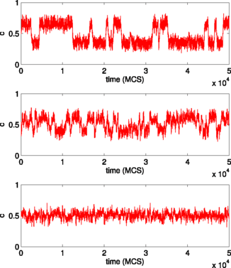
Sample trajectories showing the change of the concentration in time for the model of N=100 spinsons with anticonformity and q-lobby of size q=7. The level of anticonformity increases from upper to bottom row and p=0.35,0.4,0.5 respectively
As seen from the bottom panel of Fig. 4 for the large value of nonconformity p there is no majority in the system and c fluctuates around 0.5. For smaller values of p there is a majority in the system and spontaneous transitions between two states appear.
Spontaneous transitions between two states may look intriguing—for a relatively long time ↑-spinsons are in the majority and then suddenly, without any reason, there is a rapid change and ↓-spinsons become the majority. These sudden transitions are related to the fluctuations and therefore are less probable in larger systems. Resistance time in a given state increases, and fluctuations decrease with the size of the society N. For the infinite system spontaneous transitions are not observed and the concentration reaches one of the stationary values with the probability depending on the initial state.

6.2 Probability Density Function of the Concentration
Probability of a state with a given concentration c is described by the probability density function ρ(c,t), where t denotes time. Because initially concentration of ↑-spinsons is c 0, at time t=0 the density ρ(c,t) consists of a single peak at c=c 0 and is equal zero elsewhere. Then the system evolves according to the one of above algorithms, which means that the state of the system, and simultaneously ρ(c,t), changes. The time evolution of ρ(c,t) can be obtained from the master equation, which is kind of a ‘gain and loss’ formula [19]. Because in a single time step Δ t , three events are possible—the concentration c of ↑-spinsons increases or decreases by Δ N =1/N or remains constant:

the master equation takes form:

Above equation may look complicated for some readers, but as we have already written it is a kind of a ‘gain and loss’ equation—some events increases the probability that the concentration of ↑-spinsons increases (these events take place with probability γ +), other events decreases this probability (these events take place with probability γ −). Therefore the above equation is simply a recipe for calculating the state of the system at time t. For the infinite system probabilities γ +(c),γ −(c),γ 0(c) take particularly simple form that were already presented in [10]:
- (A):
-
In the case of anticonformity (Model A in Fig. 3):
 (8)
(8) - (B):
-
whereas in the case with independence (Model B in Fig. 3):
 (9)
(9)


It is also possible to give formulas in a case of a finite system, but since they are longer and were already presented in [10], we have decided to not repeat them here. Generally, this is not an easy task to solve analytically equation (7), but it can be done relatively easy numerically. Solving the equation, we see that the state of the system changes in time and eventually reaches a certain steady state in which ρ(c,t)=ρ(c) does not change anymore.
As already written:
-
If the probability of nonconformity p=0 then eventually system reaches a steady state in which all spinsons are ‘up’ or all spinsons are ‘down’.
In such a case stationary probability density function ρ(c) consists of two peaks at c=0 and c=1 and is equal zero elsewhere.
-
If the level of nonconformity is very large p→1 there is no majority in the system, i.e. c=0.5 in the steady state (disorder). In such a case ρ(c) consists of a single peak at c=1/2 and is equal zero elsewhere.
In Fig. 5 we have illustrated how ρ(c) changes with the level of nonconformity p for the system of N=200 spinsons and parameter q=7. As expected, for small values of p the system is polarized and for large values of p there is no majority in the system.

Stationary probability density function of the concentration of ↑-spinsons for the q-voter model with anticonformity (upper row) and independence (bottom row) for a system of N=200 individuals and a lobby size of q=7
The transition between the state with and without majority is qualitatively different in the case of anticonformity than in the case of independence.
- (A):
-
For anticonformity with increasing p maxima become lower and approach each other. Eventually they form a single maximum at c=0.5 for p=p ∗. This is a typical behavior for a continuous phase transition [47]. The critical value p ∗ increases with q and has been found analytically in [10] as p ∗(q)=(q−1)/2q.
- (B):
-
In the case with independence, for p=p ∗(q) the third maximum appears at c=0.5 (no majority). This maximum increases with p, while the remaining two maxima decrease. This is a typical behavior for a discontinuous phase transition for which we can observe the phase coexistence [47]. The critical value p ∗(q) decreases with q and has been found analytically in [10] as p ∗(q)=(q−1)/(q−1+2q−1).
6.3 Results for the Large System
As we have already mentioned, with the increasing system size N fluctuations decrease. This can be seen also from ρ(c). With increasing N peaks in Fig. 5 become more narrow and higher but do not shift in respect to c. Therefore, the stationary concentrations can be easily derived from considering the infinite system. In the stationary state the probability of growth γ + should be equal to the probability of loss γ −:
To calculate stationary values of concentration we simply solve the above equation. More detailed calculations can be found in [10] and here we present results only as a figure—dependencies between steady values of concentration c and the level of the nonconformity p for the q-voter model with anticonformity (Model A in Fig. 3) and independence (Model B in Fig. 3) are presented in Fig. 6.

Dependencies between steady values of concentration c and the level of the nonconformity p for the model with anticonformity (left panel) and independence (right panel) in the case of the q-voter model. Solid lines correspond to the stable steady states that are eventually reached. For the initial value of concentration c 0>0.5 the upper branch is reached, whereas for c 0<0.5 the lower branch is reached. Dotted lines, that are visible in a case with independence, denote unstable steady states—if the concentration is equal to the concentration denoted by the dotted line the system will not evolve. However, if the concentration is above or below the dotted line, the system will evolve towards stationary concentration denoted by the solid lines. It is seen that the value of the transition point p ∗ between the phase with majority (i.e. c≠0.5) and without majority (i.e. c=0.5) increases for the model with anticonformity and decreases for the model with independence
Two main differences are seen between Models A and B:
-
First of all, the value of the transition point p ∗ between the phase with the majority (i.e. c≠0.5) and without majority (i.e. c=0.5) increases for the model with anticonformity and decreases for the model with independence. This behavior can be easily explained recalling that both conformity and anticonformity depend on the state of the q-lobby, whereas independence does not. When q increases it becomes unlikely to choose randomly q parallel spinsons and therefore the independence term dominates. On the other hand, anticonformity takes place only when q+1 parallel spinsons are chosen randomly. Therefore the anticonformity term decline in importance more than conformity and p ∗ increases with q.
-
The second difference between models is related to the type of the phase transition. There is a continuous phase transition for an arbitrary value of q≥2 in a case of anticonformity, whereas in a case with independence the transition becomes discontinuous for q≥6 (this has been already seen in Fig. 5). Unstable fixed point, which is represented by the dotted line (on right panel in Fig. 6), means that the system cannot escape from it without external fluctuations but simultaneously never reaches this point from the outside. Therefore, concentration evolves only towards stable values, denoted by solid lines, and it jumps between two almost fully ordered states. This is very different from the behavior observed in the case with anticonformity (left panel in Fig. 6) where the concentration changes continuously. From the social point of view it means that, in the case with independence, very dramatic change of public opinion can take place with the small change of the independence level (for q≤6). In the case with anticonformity such a rapid change is not observed. From this point of view independence is more ‘dangerous’ for the social system than anticonformity, in a sense that it can cause more unexpected changes in the society.
One should remember that the differences between anticonformity and independence, that are described above, are observed merely within the q-voter model presented in Fig. 3. Therefore at least two questions naturally arise:
-
1.
Are these differences observed within other models?
-
2.
What is observed in real social systems?
The second question is obviously more important that the first one. Simultaneously, to be really fair with answering the second question, one should design and conduct adequate social experiment which is a very difficult task. Therefore, in this paper we will try at least to answer the first question. As already mentioned in the Introduction, we will not consider all possible models of opinion dynamics. Instead, we will consider a generalized q-voter model that as a special cases includes a nonlinear q-voter model, a certain type of a majority rule and also other cases that have not been considered up till now in the literature.
7 Generalized q-Voter Model
Again we consider a set of N spinsons and at each elementary time step we choose randomly q-lobby, i.e. a group of q spinsons S 1,…,S q . Then we choose randomly a voter S q+1 on which the group can influence. In the q-voter model conformity and anticonformity take place only if the q-lobby is homogeneous, i.e. all q spinsons are parallel.
In the generalized q-voter model conformity takes place if at least r spinsons among q are parallel, with the assumption that r∈[⌈q/2⌉,q], where ceiling ⌈x⌉ is the smallest integer not less than x. This assumption is made to make the model reasonable from the social point of view. The generalized model includes, as a special cases, the basic q-voter model and the majority rule:
-
For r=q the model reduces to the q-voter model presented in the previous section, i.e. unanimous majority is needed.
-
For r=⌈q/2⌉ we deal with a kind of the majority rule. In this case the majority that consists of at least half of the q-lobby is enough for the social influence. This is an idea introduced by Galam [20], although the algorithm is different since in our model only one voter changes the state instead of a whole group.
Now we are ready to introduce two types of nonconformity—anticonformity and independence:
- (A′):
-
The most natural way is to introduce anticonformity analogously to the conformity, i.e. it takes place if at least r spinsons among q are parallel. However, this is only one of the possibilities—we will call this kind of nonconformity r-anticonformity.
- (A):
-
Another possibility is to introduce anticonformity exactly in a way it was done in the q-voter model, i.e. anticonformity takes place only if all q spinsons are parallel. This assumption could be justified by the statement that the main source of anticonformity is the asserting of uniqueness (see Sect. 2).
- (B):
-
This is quite obvious how to introduce independence—spinson changes its state independently of a q-lobby, i.e. analogously as in a q-voter model.
Because it is not entirely clear how the anticonformity should be introduced we will investigate both types (see the illustration of the model in Fig. 7).

Illustration of the generalized q-voter model with the threshold r in the case of anticonformity (Models A and A′) and independence (Model B). At each elementary time step q spinsons are picked at random and form a group of influence (q-lobby). Then the voter, on which the group can influence, is randomly chosen. With probability p voter behaves like anticonformist or independent and with the probability 1−p like conformist. In this model conformity takes place if at least r spinsons in the q-lobby are in the same state. To make the model as general as possible two types of anticonformity are proposed:
(A) The first type of anticonformity (Model A) is identical as in the q-voter model—it takes place only if the q-lobby is homogeneous.
(A′) The second type, so called r-anticonformity (Model A′), acts in the same way as conformity—it takes place if at least r spinsons in the q-lobby are in the same state.
(B) In a case of independent behavior, the voter does not follow the group, but acts independently—with probability 1/2 it flips to the opposite direction.
To make the model reasonable from the social point of view we will consider r∈[⌈q/2⌉,q], where ceiling ⌈x⌉ is the smallest integer not less than x. For r=q the model reduces to the q-voter model presented in Fig. 3. In such a case Model A is equivalent with A′. For r=⌈q/2⌉ we deal with a kind of the majority rule—at least half of the group has to be in the same state to influence the voter
In the q-voter model there are only two parameters—the probability of nonconformity p and the size of the group q. In the generalized q-voter model additionally there is a third parameter—the threshold r. Therefore analysis is a bit more complicated but nevertheless we are able, as in a case of the q-voter model, find the stationary behavior of the system. Again stationary values of concentration c can be derived relatively easily for the infinite system.
The probability that the number of ↑-spinsons increases in a single time step is given by:
where α ↑ denotes the probability that the number of ↑-spinsons increases due to the conformity and β ↑ denotes the probability that the number of ↑-spinsons increases due to the one of two possible types of nonconformity (anti-conformity or independence). Analogously, the probability that the number of ↓-spinsons increases (which is equivalent to the probability that the number of ↑-spinsons decreases) in a single time step is given by:
where α ↓ denotes the probability that the number of ↓-spinsons increases due to the conformity and β ↓ denotes the probability that the number of ↓-spinsons increases due to the one of two possible types of nonconformity. Of course there is also nonzero probability that nothing changes:
Probabilities that the number of ↑-spinsons increases or decreases due to the conformity can be calculated as:


whereases probabilities that the number of ↑-spinsons increases or decreases due to the nonconformity depends on a type of nonconformity:
- (A′):
-
In the case of r-anticonformity (see Model A′ in Fig. 7):
 (16)
(16) (17)
(17) - (A):
-
In the case of anticonformity like in the original q-voter model (see Model A in Fig. 7):
 (18)
(18) (19)
(19) - (B):
-
In the case of independence (see Model B in Fig. 7):
 (20)
(20) (21)
(21)


Again we find the stationary values of concentration from the condition γ +−γ −=0.
7.1 The Majority Case
We begin with presenting results for the majority case, i.e. for r=⌈q/2⌉ (see Fig. 8). It is seen that dependencies between c and p for various types of nonconformity do not differ as much as they did in the case of the q-voter model (see Fig. 6). In all three cases the continuous phase transition between states with majority and without majority is observed. Moreover, in all three cases the value of the transition point increases with the size of the q-lobby.

Dependencies between steady values of concentration c and the level of the nonconformity p for the model with anticonformity, r-anticonformity and independence in the case of the majority rule, i.e. r=⌈q/2⌉. As seen, in contrast to the q-voter model (i.e. r=q), results are qualitatively the same for all types of nonconformity. In all three cases there is a continuous phase transition between states with and without majority and the value of the transition point increases with q. This means that within majority rule we do not observe, on the macroscopic scale, any qualitative differences between various types of nonconformity
7.2 The General Case
Now we move to the general case with q>0 and r∈[⌈q/2⌉,q]. Dependencies between c and p for a fixed value of q=9 and different values of r are presented in Fig. 9. In this case results for three types of nonconformity are qualitatively different. As usually, there is an order-disorder phase transition at p=p ∗. However, the type of the phase transition is different for independence than in the cases with anticonformity. For a critical value of r=r ∗(q), that scales almost linearly with q, the transition changes its type from continuous to discontinuous. We should stress here that such a behavior is observed only for the size of the q-lobby q≥6. For q=6 there is a discontinuous phase transition only for the threshold r=6 (i.e. the case of the q-voter model). For the size of the lobby q=7 still a discontinuous phase transition is observed only for r=q=7. For q=9 a discontinuous phase transition is observed for r=8 and r=9, i.e. r ∗(9)=8 and for q=12 a discontinuous phase transition is observed for r=10,11,12, i.e. r ∗(12)=10. It is also seen in Fig. 9 that the value of the phase transition point p ∗ between state with majority (i.e. c≠0.5) and without majority (c=0.5) increases for r-anticonformity and decreases for anticonformity and independence. This can be understood also heuristically and we will return to this issue later.

Dependencies between steady values of concentration c and the level of nonconformity p for the q-voter model with the threshold r for three types of nonconformity: anticonformity, r-anticonformity and independence. In all cases q=9 and the threshold r∈[⌈q/2⌉,q]. Although in all three cases there is a phase transition, there are qualitative differences between three types of nonconformity. As usually, solid lines correspond to the stable steady states and dotted lines, that are visible in a case with independence, denote unstable steady states.
(A′) In the case with r-anticonformity the phase transition is continuous and p ∗ decreases with r.
(A) In the case with anticonformity the phase transition is continuous and the critical point p ∗ increases with r.
(B) In the case of independence the phase transition changes its character from continuous to discontinuous for q≥6 and r≥r ∗(q) that grows almost linearly with q. For example: r ∗(q=6)=6,r ∗(q=9)=8,r ∗(q=12)=10,r ∗(q=20)=14 and approximately satisfies the equation q=1.8r ∗−4.9
8 The Phase Diagrams for the Generalized q-Voter Model
In Figs. 6, 7, 8 and 9 we have presented dependencies between stationary values of concentration and the level of nonconformity. As has been already noted in [28] both types of nonconformity, anticonformity and independence, tend to be effective in differentiating people from others. Indeed, within our model, all three types of nonconformity lead to the phase transition between consensus and stalemate (in a sense that there is no majority in the system).
However, the type of the phase transition and the dependence between the critical value p ∗ and parameters q,r depends strongly on the type of nonconformity. Therefore, to summarize all results we construct and discuss the phase diagrams for all types of nonconformity. The critical value of nonconformity, below which there is a majority in the system, can be calculated as:

where α ↑,α ↓ are given by Eq. (15) and β ↑,β ↓ are given by Eqs. (19), (17), (21) respectively to the type of nonconformity. Intentionally, we do not present here any calculations, since the paper is intended to be available for a wide range of readers. However, the procedure is the same as in the case of the q-voter model, for which detailed calculations can be found in [10].
8.1 The Special Cases—Unanimity and Majority
Let us start with two special cases—‘unanimity’ (i.e. r=q) and ‘majority’ (i.e. ⌈q/2⌉). These two cases are particularly simple because r is uniquely determined by q and therefore the critical value of nonconformity p ∗ depends only on the single parameter q. Phase diagrams for these cases are presented in Fig. 10. As already seen in Figs. 6 and 8:
-
In the case of the majority the critical value p ∗ grows with q for all three types of nonconformity. The phase transition is continuous for arbitrary value of q≥2.
-
In contrast, in the case of the ‘unanimity’ (r=q) the critical value of nonconformity p ∗ increases for anticonformity and decreases for independence.
Moreover, in the case of independence there is a discontinuous phase transition for q≥6, which is denoted by a region of a coexistence. In the coexistence region one of two phases (with or without majority) is metastable and the second one is stable.
The system can reach metastable state but larger fluctuations can easily derive the system from this state. Therefore, the probability of reaching such a state is lower than probability of reaching the stable state. At the transition point, denoted in Fig. 10 by the dashed line—both states are equally probable, i.e. both states are stable.
Fig. 10 
Phase diagrams for the model with the majority rule, i.e. r=⌈q/2⌉ (upper panels) and the q-voter model, i.e. r=q (bottom panels).
(A′) For r-anticonformity the majority is equivalent to unanimity. There is a continuous phase transition and the critical value p ∗ grows with q. In this case the majority is equivalent to unanimity.
(A) For anticonformity in both cases there is a continuous phase transition and the critical value p ∗ increases with q.
(B) For independence, in the case of the majority the critical value p ∗ increases with q, whereas in the case of the ‘unanimity’ (r=q) decreases. Moreover, in the case of independence there is a discontinuous phase transition for q≥6, which is denoted by a region of a coexistence. In the coexistence region one of two phases (with or without majority) is metastable and the second one is stable. The system can reach metastable state but larger fluctuations can easily derive the system from this state. Therefore, the probability of reaching such a state is lower than probability of reaching the stable state. At the transition point, denoted in Fig. 10 by the dashed line—both states are equally probable, i.e. both states are stable

Results presented up till now have shown that:
-
The difference between anticonformity and independence, that is introduced on the microscopic (psychological) level, can influence the behavior on the macroscopic (society) scale.
-
Within the presented model, the macroscopic behavior of the system is much richer if we assume that the social influence takes place in the case of unanimous instead absolute majority.
8.2 The General Case
Now we construct the phase diagram in the general case in which r∈[⌈q/2⌉,q]. In such a case the critical value p ∗ depends on two parameters q and r. Therefore, we fist present the phase diagram for a chosen fixed values of q=15 and q=20 (see Fig. 11). We have chosen these values of q just as an example—the complete 3-dimensional phase diagram is far less legible. Qualitative differences are seen between three types of nonconformity:
- (A′):
-
There is a continuous phase transition in the case of r-anticonformity (Model A′ in Fig. 7) and the critical value of p decreases with r.
- (A):
-
For anticonformity (Model A in Fig. 7) the phase transition is also continuous but the critical value of p increases with r.
- (B):
-
In the case with independence (Model B in Fig. 7) the critical value of p decreases with r and the transition changes its character from continuous to discontinuous.

Phase diagrams for the generalized q-voter model with a threshold r for the fixed values of q=15 (upper panels) and q=20 (bottom panels). Qualitative differences are seen between three types of nonconformity:
(A′) There is a continuous phase transition in the case of r-anticonformity (Model A′ in Fig. 7) and the critical value of p decreases with r.
(A) For anticonformity (Model A in Fig. 7) the phase transition is also continuous but the critical value of p increases with r.
(B) In the case with independence (Model B in Fig. 7) the critical value of p decreases with r and the transition changes its character from continuous to discontinuous
The dependence between a critical value of p and parameter r can be not only calculated analytically or numerically but also heuristically explained:
- (A′):
-
For a given size of the lobby q r-anticonformity decreases with r faster than conformity. While conformity takes place if r spinsons inside the q-lobby are parallel, r-anticonformity demands r+1 parallel spinsons.
- (A):
-
Anticonformity takes place only if q+1 spinsons are parallel, i.e. does not depend on r. On the other hand conformity is decreasing with increasing r because when r grows it becomes unlikely to find r parallel spinsons inside the q-lobby. Therefore, p ∗ should decrease with r, what is indeed observed.
- (B):
-
It is also easy to understand why p ∗ decreases with r in the case of independence—this type of nonconformity does not depend on the state of q-lobby. On the other hand, as explained above, conformity is decreasing with increasing r.
Now we investigate the dependence p ∗(q) for a fixed value of r. In Fig. 12 the phase diagram is presented for a sample values of r=10 and r=15. Again, qualitative differences are seen between three types of nonconformity:
- (A′):
-
In the case of r-anticonformity there is a continuous order-disorder transition and the critical value of p decreases with q.
- (A):
-
For anticonformity there is no phase transition—the system is ordered for arbitrary value of q.
- (B):
-
Finally, in the case with nonconformity the critical value of p increases with q and the transition changes its character from discontinuous to continuous.

Phase diagrams for the generalized q-voter model with a threshold r for the fixed values of r=15 (upper panels) and r=10 (bottom panels). Qualitative differences are seen between three types of nonconformity:
(A′) In the case of r-anticonformity there is a continuous order-disorder transition and the critical value of p decreases with q.
(A) For anticonformity there is no phase transition—the system is ordered for arbitrary value of q.
(B) Finally, in the case with nonconformity the critical value of p increases with q and the transition changes its character from discontinuous to continuous
Again, we can try to understand heuristically dependencies between critical values of p and parameter q:
- (A′):
-
For a given r conformity is increasing with q, since it is easier to find r parallel spinsons in the q-lobby if q is larger. Obviously r-anticonformity, similarly to conformity, becomes more probable with increasing q. The question is which force, conformity or r-anticonformity, grows faster with q. It can be easily checked that r-anticonformity gain more with q because it takes place if at least r+1 spinsons are parallel among q+1, whereas conformity takes place if at least r spinsons are parallel among q. Therefore p ∗ decreases with q in this cases.
- (A):
-
Far less intuitive is the case with anticonformity. It is obvious that anticonformity decreases with q because it takes place only if q+1 spinsons are parallel. Therefore we have a competition of two forces—conformity increases with q and anticonformity decreases. It occurs that this competition results in constant value of p ∗=1—i.e. for any value of q there is a majority in the system.
- (B):
-
Because for a given r conformity is increasing with q it is easy to understand why p ∗ increases with q in the case of independence—this type of nonconformity does not depend on the state of q-lobby.
9 Summary
The main goal of this paper was to examine how different types of nonconformity, introduced on the microscopic level, manifest at the level of the society (i.e. macroscopic). Moreover, we wanted to check if results would be universal or rather model-dependent. To achieve the goal we have introduced a generalized q-voter model. There are three parameters in the model:
-
1.
q—the size of the q-lobby, i.e. the size of a group of influence,
-
2.
p—the level (probability) of nonconformity that can be one of two types—anticonformity or independence,
-
3.
r—the threshold needed for social influence (e.g. conformity takes place if at least r spinsons among q are parallel).
All these parameters are important, but each for a different reason:
- (q):
-
By varying q, we can move from a linear voter model to a nonlinear voter models of different orders (including Sznajd model for q=2).
- (p):
-
p introduced a noise to the system—both types of nonconformity destroy order, although each in a slightly different way. By varying p we move from the complete consensus to the status-quo situation.
- (r):
-
The parameter r allows for the unification of several opinion dynamics models—e.g. for r=⌈q/2⌉ we deal with the majority model and for r=q with the original q-voter model. From this point of view the threshold r is not so important from the social point of view, but is used rather to understand how details of the model (in this case the way of introducing conformity) affect results. On the other hand it may be also connected with the level of majority that is needed to persuade.
We would like to emphasize that we are aware of the fact that the parameter space for agent-based models is much richer than the 3-parameter space used in this paper. However, our aim was not to propose a possibly general model of opinion formation. We wanted to check if the differences between independence and anticonformity, that were shown within the q-voter model [10], would be visible if the conformity acted not only in the case of unanimity but for example in the case of absolute majority or in other cases—and hence the idea of introducing the threshold r into the q-voter model.
Our calculations have shown that results depend significantly on parameters. In particular:
-
For the majority rule, that corresponds to r=⌈q/2⌉, there is a continuous phase transition at p=p ∗ between state with majority and status-quo for both types of nonconformity for any value of q>1. Moreover, for both types of nonconformity p ∗ increases with the size of the q-lobby. Therefore, differences between anticonformity and independence are qualitatively indistinguishable on the macroscopic level under the majority rule.
-
In the case of a q-voter model, that corresponds to r=q, there are significant differences between two types of nonconformity. In the case of anticonformity there is a continuous order–disorder phase transition at p=p ∗ and the value of p ∗ increases with the size of the q-lobby. On the other hand, for the model with independence the value of the transition point p ∗ decays with q. Moreover, the phase transition in this case is continuous only for q≤5. For larger values of q there is a discontinuous phase transition—and coexistence of ordered (with majority) and disordered (without majority) phase is possible.
-
In the general case in which r and q are two independent parameters, the differences between anticonformity and independence depends on r and q. Similarly as in the case of the q-voter model there is a continuous phase transition in the case of anticonformity, whereas in the case of independence the change of the transition’s type may appear dependently on parameters r and q.
Above results suggests that differences between anticonformity and independence might be significant or indistinguishable on the macroscopic level, depending on parameters of the model. Therefore, we are able to answer fairly questions posed in the Introduction:
-
1.
Differences between two types of nonconformity, that are recognized by social psychologists on the individual (microscopic) level, can manifest on the society (macroscopic) level within some models. For example there are significant differences between anticonformity and independence in the q-voter model in which unanimous majority is required for the social influence. Analogous results are obtained in the case when the threshold r, needed for a social influence, is high enough, which can be understood as an almost unanimous majority.
-
2.
Differences between anticonformity and independence, that manifest on the macroscopic level, are not universal. They depend on the model designs. For example in a case of majority rule two types of nonconformity are qualitatively indistinguishable.
Above answers, although complete the goal of the paper, raise further important questions related to the value and validity of opinion dynamics models. Differences on the macroscopic level, that were shown in this paper, may indicate which microscopic model is correct, and which one should be rejected. However, to judge which macroscopic behavior is adequate in the real social system might be very hard or maybe even impossible. It would be extremely valuable if one could design and conduct the social experiment which could show differences between anticonformity and independence on the macroscopic level. So far, we can only conclude that the social behavior, even in seemingly simple world of spinsons, is surprisingly complex.
References
Macy, M.W., Willer, R.: From factors to actors: computational sociology and agent-based modeling. Annu. Rev. Sociol. 28, 143–166 (2002)
Squazzoni, F.: The impact of agent-based models in the social sciences after 15 years of incursions. Hist. Econ. Ideas XVIII, 197–233 (2010)
Chen, S.: Varieties of agents in agent-based computational economics: a historical and an interdisciplinary perspective. J. Econ. Dyn. Control 36, 1–25 (2012)
Rand, W., Rust, R.T.: Agent-based modeling in marketing: guidelines for rigor. Int. J. Res. Mark. 28, 181–193 (2011)
Kiesling, E., Günther, M., Stummer, Ch., Wakolbinger, L.M.: Agent-based simulation of innovation diffusion: a review. Cent. Eur. J. Oper. Res. 20, 183–230 (2012)
Galam, S., Gefen, Y., Shapir, Y.: Sociophysics: a new approach of sociological collective behavior. I. Mean-behavior description of a strike. J. Math. Sociol. 9, 1–13 (1982)
Galam, S.: Sociophysics: a personal testimony. Physica A 336, 49–55 (2004)
Galam, S.: Sociophysics: A Physicist’s Modeling of Psycho-Political Phenomena. Springer, New York (2012)
Castellano, C., Fortunato, S., Loreto, V.: Statistical physics of social dynamics. Rev. Mod. Phys. 81, 591–646 (2009)
Nyczka, P., Sznajd-Weron, K., Cislo, J.: Phase transitions in the q-voter model with two types of stochastic driving. Phys. Rev. E 86, 011105 (2012)
Martins, A.C.R.: Discrete opinion models as a limit case of the CODA model. arXiv:1201.4565v1
Lewenstein, M., Nowak, A., Latane, B.: Statistical mechanics of social impact. Phys. Rev. A 45, 763–776 (1992)
Hołyst, J.A., Kacperski, K., Schweitzer, F.: Social impact models of opinion dynamics. Ann. Rev. Comput. Phys. 9, 253–273 (2001)
Martins, A.C.R.: Continuous opinions and discrete actions in opinion dynamics problems. Int. J. Mod. Phys. C 19, 617–624 (2008)
Axelrod, R.: The dissemination of culture: a model with local convergence and global polarization. J. Confl. Resolut. 41, 203–226 (1997)
Deffuant, G., Neau, D., Amblard, F., Weisbuch, G.: Mixing beliefs among interacting agents. Adv. Complex Syst. 3, 87–98 (2001)
Hegselmann, R., Krause, U.: Opinion dynamics and bounded confidence: models, analysis and simulation. J. Artif. Soc. Soc. Simul. 5(3) (2002). http://jasss.soc.surrey.ac.uk/5/3/2.html
Liggett, T.M.: Interacting Particle Systems. Springer, Heidelberg (1985)
Krapivsky, P.L., Redner, S., Ben-Naim, E.: A Kinetic View of Statistical Physics. Cambridge University Press, Cambridge (2010)
Galam, S.: Majority rule, hierarchical structures and democratic totalitarianism: a statistical approach. J. Math. Psychol. 30, 426–434 (1986)
Galam, S.: Social paradoxes of majority rule voting and renormalization group. J. Stat. Phys. 61, 943–951 (1990)
Krapivsky, P.L., Redner, S.: Dynamics of majority rule in two-state interacting spin systems. Phys. Rev. Lett. 90, 238701 (2003)
Sznajd-Weron, K., Sznajd, J.: Opinion evolution in closed community. Int. J. Mod. Phys. C 11, 1157–1165 (2000)
Galam, S.: Local dynamics vs. social mechanisms: a unifying frame. Europhys. Lett. 70, 705–711 (2005)
Lambiotte, R., Redner, S.: Dynamics of non-conservative voters. Europhys. Lett. 82, 18007 (2008)
Castellano, C., Muñoz, M.A., Pastor-Satorras, R.: Nonlinear q-voter model. Phys. Rev. E 80, 041129 (2009)
Cialdini, R.B., Goldstein, N.J.: Social influence: conformity and compliance. Annu. Rev. Psychol. 55, 591–621 (2004)
Griskevicius, V., Goldstein, N.J., Mortensen, C.R., Cialdini, R.B., Kenrick, D.T.: Going along versus going alone: when fundamental motives facilitate strategic (non)conformity. J. Pers. Soc. Psychol. 91, 281–294 (2006)
Latane, B.: The psychology of social impact. Am. Psychol. 36, 343–356 (1981)
Asch, S.E.: Opinions and social pressure. Sci. Am. 193, 31–35 (1955)
Pronin, E., Berger, J., Molouki, S.: Alone in a crowd of sheep: asymmetric perceptions of conformity and their roots in an introspection illusion. J. Pers. Soc. Psychol. 92, 585–595 (2007)
Murray, D.R., Trudeau, R., Schaller, M.: On the origins of cultural differences in conformity: four tests of the pathogen prevalence hypothesis. Pers. Soc. Psychol. Bull. 37, 318329 (2011)
Willis, R.H.: Two dimensions of conformity-nonconformity. Sociometry 26, 499–513 (1963)
Willis, R.H.: Conformity, independence, and anticonformity. Hum. Relat. 18, 373–388 (1965)
Nail, P., MacDonald, G., Levy, D.: Proposal of a four-dimensional model of social response. Psychol. Bull. 126, 454–470 (2000)
MacDonald, G., Nail, P.R., Levy, D.A.: Expanding the scope of the social response context model. Basic Appl. Soc. Psychol. 26, 77–92 (2004)
MacDonald, G., Nail, P.R.: Attitude change and the public-private attitude distinction. Br. J. Soc. Psychol. 44, 15–28 (2005)
Nail, P.R., MacDonald, G.: On the development of the social response context model. In: Pratkanis, A. (ed.) The Science of Social Influence: Advances and Future Progress, pp. 193–221. Psychology Press, New York (2007)
Solomon, M.R., Bamossy, G., Askegaard, S., Hogg, M.K.: Consumer Behavior, 3rd edn. Prentice Hall, New York (2006)
Brush, S.G.: History of the Lenz-Ising model. Rev. Mod. Phys. 39, 883–893 (1967)
Niss, M.: History of the Lenz-Ising model 1920–1950: from ferromagnetic to cooperative phenomena. Arch. Hist. Exact Sci. 59, 267–318 (2005)
Niss, M.: History of the Lenz-Ising model 1950–1965: from irrelevance to relevance. Arch. Hist. Exact Sci. 63, 243–287 (2009)
Niss, M.: History of the Lenz-Ising model 1965–1971: the role of a simple model in understanding critical phenomena. Arch. Hist. Exact Sci. 65, 625–658 (2011)
Galam, S.: Fragmentation versus stability in bimodal coalitions. Physica A 230, 174–188 (1996)
Galam, S., Moscovici, S.: Towards a theory of collective phenomena: consensus and attitude changes in groups. Eur. J. Soc. Psychol. 21, 49–74 (1991)
Galam, S.: Rational group decision making: a random field Ising model at T=0. Physica A 238, 66–80 (1997)
Callen, H.B.: Thermodynamics and an Introduction to Thermostatics, 2nd edn. Wiley, New York (1985)
Schelling, T.C.: Dynamic models of segregation. J. Math. Sociol. 1, 143–186 (1971)
Kawasaki, K.: Kinetics of Ising models. In: Domb, C., Green, M.S. (eds.) Phase Transitions and Critical Phenomena, vol. 2, pp. 443–501. Academic Press, San Diego (1972)
Goldenberg, J., Efroni, S.: Using cellular automata modeling of the emergence of innovations. Technol. Forecast. Soc. Change 68, 293–308 (2001)
Goldenberg, J., Libai, B., Muller, E.: Using complex systems analysis to advance marketing theory development: modeling heterogeneity effects on new product growth. Acad. Market. Sci. Rev. 9, 1–18 (2001)
Garber, T., Goldenberg, J., Libai, B., Muller, E.: From density to destiny: using spatial dimension of sales data for early prediction of new product success. Mark. Sci. 23, 419–428 (2004)
Moldovan, S., Goldenberg, J.: Cellular automata modeling of resistance to innovations: effects and solutions. Technol. Forecast. Soc. Change 71, 425–442 (2004)
Wu, F.Y.: The Potts model. Rev. Mod. Phys. 54, 235–268 (1982)
Deffuant, G., Huet, S., Amblard, F.: An individual-based model of innovation diffusion mixing social value and individual benefit. Am. J. Sociol. 110, 1041–1069 (2005)
Thiriot, S., Kant, J.D.: Using associative networks to represent adopters’ beliefs in a multiagent model of innovation diffusion. Adv. Complex Syst. 11, 261–272 (2008)
Kosterlitz, J.M., Thouless, D.J.: Ordering, metastability and phase transitions in two-dimensional systems. J. Phys. C, Solid State Phys. 6, 1181–1203 (1973)
Kosterlitz, J.M.: The critical properties of the two-dimensional xy model. J. Phys. C, Solid State Phys. 7, 1046–1060 (1974)
Flache, A., Macy, M.W.: Small worlds and cultural polarization. J. Math. Sociol. 35, 146–176 (2011)
Deffuant, G., Neau, D., Amblard, F., Weisbuch, G.: Adv. Complex Syst. 3, 87 (2000)
Ashkin, J., Teller, E.: Statistics of two-dimensional lattices with four components. Phys. Rev. 64, 178 (1943)
Sznajd-Weron, K., Sznajd, J.: Who is left, who is right? Physica A 351, 593 (2005)
Mobilia, M.: Does a single zealot affect an infinite group of voters? Phys. Rev. Lett. 91, 028701 (2003)
Galam, S.: Contrarian deterministic effects on opinion dynamics: the hung elections scenario. Physica A 333, 453–460 (2004)
Schneider, J.: The influence of contrarians and opportunists on the stability of a democracy in the Sznajd model. Int. J. Mod. Phys. C 15, 659–674 (2004)
de la Lama, M.S., Lopez, J.M., Wio, H.S.: Spontaneous emergence of contrarian-like behavior in an opinion spreading model. Europhys. Lett. 72, 851–857 (2005)
Galam, S., Jacobs, F.: The role of inflexible minorities in the breaking of democratic opinion dynamics. Physica A 381, 366–376 (2007)
Sznajd-Weron, K., Tabiszewski, M., Timpanaro, A.M.: Phase transition in the Sznajd model with independence. Europhys. Lett. 96, 48002 (2011)
Albert, R., Barabasi, A.L.: Statistical mechanics of complex networks. Rev. Mod. Phys. 74, 47–97 (2002)
Watts, D.J.: The “new” science of networks. Annu. Rev. Sociol. 30, 243–270 (2004)
Dorogovtsev, S.N., Goltsev, A.V., Mendes, J.F.F.: Critical phenomena in complex networks. Rev. Mod. Phys. 80, 1275–1335 (2008)
Merton, R.K.: Social Theory and Social Structure. Free Press, New York (1968)
Conley, D.: You May Ask Yourself: An Introduction to Thinking Like a Sociologist, 2nd edn. Norton, New York (2011)
Sznajd-Weron, K., Weron, R.: A simple model of price formation. Int. J. Mod. Phys. C 13, 115–123 (2002)
Slanina, F., Lavicka, H.: Analytical results for the Sznajd model of opinion formation. Eur. Phys. J. B 35, 279 (2003)
Author information
Authors and Affiliations
Corresponding author
Additional information
The work was supported by funds from the National Science Centre (NCN) through grant no. 2011/01/B/ST3/00727.
Rights and permissions
About this article
Cite this article
Nyczka, P., Sznajd-Weron, K. Anticonformity or Independence?—Insights from Statistical Physics. J Stat Phys 151, 174–202 (2013). https://doi.org/10.1007/s10955-013-0701-4
Received:
Accepted:
Published:
Issue Date:
DOI: https://doi.org/10.1007/s10955-013-0701-4