A Central Limit Theorem for Time-Dependent Dynamical Systems

Abstract

The work by Ott et al. (Math. Res. Lett. 16:463–475, 2009) established memory loss in the time-dependent (non-random) case of uniformly expanding maps of the interval. Here we find conditions under which we have convergence to the normal distribution of the appropriately scaled Birkhoff-like partial sums of appropriate test functions. A substantial part of the problem is to ensure that the variances of the partial sums tend to infinity (cf. the zero-cohomology condition in the autonomous case). In fact, the present paper is the first one where non-random examples are also found, which are not small perturbations of a given map. Our approach uses martingale approximation technique in the form of Sethuraman and Varadhan (Electron. J. Probab. 10:121–1235, 2005).

1 Introduction

Time-dependent dynamical systems appear in various applications. Recently, [12] could establish exponential loss of memory for expanding maps and, moreover, for one-dimensional piecewise expanding maps with slowly varying parameters. It also provided interesting motivations and examples for the problem. We also mention that the memory loss result of [12] has been extended very recently to two dimensional Anosov diffeomorphisms in [14]. For us—beside their work—an additional incentive was the question of J. Lebowitz [10]: bound the correlation decay for a planar finite-horizon Lorentz process which is periodic apart form the 0-th cell; in it, the Lorentz particle encounters a particular scatterer of the 0-th cell moderately displaced at its each subsequent return to the 0-th cell. (Slightly similar is the situation in the Chernov-Dolgopyat model of Brownian motion, where—between subsequent collisions of the light particle with the heavy one—the heavy particle slightly moves away, cf. [4].)

The results of [12] say that—for sequences of uniformly expanding maps—distances of images of a pair of different initial measures converge to 0 exponentially fast. In the same setup it is also natural to expect that probability laws of the Birkhoff-type partial sums of some given function—scaled, of course, by the square roots of their variances—are approximately Gaussian. The main theorem of our paper provides a positive answer though our conditions are surprisingly more restrictive than those of [12]. Let us explain the difficulty and some related results.

In functional central limit theorems for functions of autonomous chaotic deterministic systems the zero-cohomology condition is—in quite a generality—known to be necessary and sufficient for the vanishing of the limiting variance (see [11] for instance). For time-dependent systems, however, such a condition is only known for almost all versions of random dynamical systems (see [1] and [5]) and for other models the situation can be and definitely is completely different. In fact, for time-dependent systems, first [2, 3] had proved a Gaussian approximation theorem in quite a generality; its author, however, assumed that the variances of the Birkhoff-type partial sums tend to ∞ sufficiently fast; the paper, however, did not provide any example when this condition would hold. The more recent work [6] proves under some reasonable conditions a dichotomy: either the variances are bounded or the Gaussian approximation holds; the article also provides an example for the latter in the case when the time dependent maps are smaller and smaller perturbations of a given map. But still there is no general method for ascertaining whether the variance is bounded or not. Finally we note that [8, 9] has interesting results for higher order cohomologies but its setup is different.

The present work is, in fact, the first one where non-random examples are also found, that are not small perturbations of a given map. The proof of our main theorem uses martingale approximation technique in the form introduced in [13] for treating additive functions of inhomogeneous Markov chains. The organization of our paper is simple: its Sect. 2 contains our main theorem and provides examples when it is applicable. Section 3 is devoted to the proof of the theorem.

2 Results

Let A be a set of numbers and $(X, \mathcal{F}, \mu)$ a probability space. For each a∈A define T _a :X→X. Suppose that μ is invariant for all T _a ’s. Now consider a sequence of numbers from A, i.e. $\underline{a}: \mathbb{N} \rightarrow A$. Our aim is to prove some kind of central limit theorem for the sequence

with some nice function f:X→ℝ.

As usual,

and $\hat{T}^{*}$ is the L ²(μ)-adjoint of $\hat{T}$ (the so-called Perron-Frobenius operator). Further, introduce the notation

and for simplicity write $\hat{T}_{[j]} = \hat{T}_{[1..j]}$.

Similarly, define

and $\hat{T}_{[j]}^{*} = \hat{T}_{[1..j]}^{*}$.

Further, define σ-algebras $\mathcal{F}_{0} = \mathcal{F}$, $\mathcal{F}_{i} = (T_{a_{1}})^{-1} \dots(T_{a_{i}})^{-1} \mathcal{F}_{0}$. We will need this sequence of σ-algebras to form a decreasing systems (cf. Assumption 2 of Theorem 1), restricting our approach to non-invertible maps. Let us assume that there is a Banach space $\mathcal{B}$ of $\mathcal{F}$-measurable functions on X such that $\| g \| := \| g \|_{\mathcal{B}} \geq\| g\|_{\infty}$ for all $g \in\mathcal{B}$.

Finally, for the fixed function f, introduce the notation

With the above notation, our aim is to prove a limit theorem for $S_{n}(x) = \sum_{k=1}^{n} \hat{T}_{[k]} f(x)$.

Theorem 1

Assume that f, $\underline{a}$ and T _b , b∈A satisfy the following assumptions.

• 1. ∫fdμ=0.

• 2. T _b is onto but not invertible for all b∈A.

• 3. $f \in\mathcal{B}$ and there exist K<∞ and τ<1 such that for all sequences $\underline{b}$ and for all k, $\| \hat {T}_{b_{1}}^{*} \ldots \hat{T}_{b_{k}}^{*} f \| < K \tau^{k} \| f \|$.

• 4. (Accumulated transversality) Define χ _k as the L ²-angle between u _k and the subspace of $(T_{a_{k+1}})^{-1} \mathcal{F}_{0}$-measurable functions. Then

  

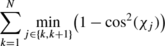
  converges to ∞ as N→∞.

Then

and

converges weakly to the standard normal distribution, where x is distributed according to μ.

Assumption 3 roughly tells that there is an eventual spectral gap of the operators $\hat{T}_{a_{j}}^{*}$ which is quite a natural assumption. Assumption 4 guarantees that there is no much cancellation in S _n , for instance f cannot be in the cohomology class of the zero function when |A|=1.

Before proving the statement let us examine a special case.

Example 1

Define $(X, \mathcal{F}, \mu) = (S^{1}, \mbox{Borel}, \mbox{Leb})$, A={2,3,…}, T _a (x)=ax (mod 1), $\mathcal{B} = C^{1}=C^{1}(S^{1})$,

Fix a non constant function f∈C ¹ satisfying ∫fdx=0. Then there exists some integer L=L(f) such that with all sequences $\underline{a}$ for which

the assumptions of Theorem 1 are fulfilled.

Proof of Example 1

It is easy to see that for all g∈C ¹ with zero mean, and for all $\underline{b} : \mathbb{N} \rightarrow A$,

and similarly,

(1)

Hence Assumption 3 is fulfilled.

In order to check Assumption 4, select x,y∈S ¹, ε>0,δ>0 such that

This can be done since f is not constant. Now choose

Whence

Thus if a _k >L, then

is true independently of the choice of a ₁,…,a _k−1. This yields

Since $L>\frac{2}{ \varepsilon}$, for all g which is $( T_{a_{k+1}})^{-1} \mathcal{F}_{0}$ measurable (with a _k+1>L), one can find h:[0,ε/2)→ℝ and ε ₁≤ε/2 such that g(y+ε ₁+z)=g(x+z)=h(z) for all z∈[0,ε/2). Hence,

(2)

Since

is bounded, (2) implies that (1−cos²(χ _k )) is uniformly bounded away from zero if min{a _k ,a _k+1}>L.

Hence, Assumption 4 is fulfilled if there exist infinitely many indices k such that

 □

In Example 1, expanding maps with large derivative were needed in order to obtain the Gaussian approximation. Naturally arises the question that what happens in the case when one uses only finitely many dynamics, for instance, only T ₂ and T ₃ of Example 1. That is why we discuss the following example.

Example 2

Define $X, \mathcal{F}, \mu, A, T_{b}, \mathcal{B}$ as in Example 1. If $\underline{a}$ is a sequence for which there is a b∈A such that for all integer K, one can find a k for which

and $f \in\mathcal{B}$, ∫f=0 is any function for which the equation $f = \hat{T}_{b} u - u$ has no solution u, then the assumptions of Theorem 1 are fulfilled.

Proof of Example 2

It is enough to verify Assumption 4. To do so, for K∈ℤ₊ pick k such that

(3)

Then (1) implies that

(4)

holds for j=k,k+1 with some C uniformly in K. Now, if $g := \sum_{i=0}^{\infty} ( \hat{T}_{b}^{*} )^{i} f$ is not $(T_{b})^{-1} \mathcal{F}_{0}$-measurable, then necessarily its L ²-angle with those functions is positive. Since (3) and (4) hold for infinitely many k’s, min{χ _k ,χ _k+1} exceeds a uniform positive number infinitely many times, inferring Assumption 4. On the other hand, if g is $(T_{b})^{-1} \mathcal{F}_{0}$-measurable, then $g = \hat{T}_{b}\hat{T}_{b}^{*}g$ and $g- \hat{T}_{b}^{*}g = f$ imply that for $u= \hat{T}_{b}^{*}g$, $\hat{T}_{b} u - u =f$. □

Note, that in Example 2, Var(S _n ) can be arbitrarily small. Indeed, pick a C ¹ function f, for which $f = \hat{T}_{3} u - u$ has no solution u, but there is some v such that $f = \hat{T}_{2} v - v$. Now, pick a sequence of integers d _l ,l∈ℕ, d _l →∞ fast enough, and define

It is easy to see that (1) implies $\mathbb{E}(|\hat{T}_{[i]}f \cdot\hat{T}_{[j]}f|) \leq2^{|i-j|+1}\|f\|^{2}$ (formally it follows from (16)), which in turn yields that Var(S _k ) is bounded by some constant times k. Now, with the notation l _n :=max{l:d _l ≤n}, write

On the other hand, $f = \hat{T}_{2} v - v$ implies that $\hat{T}_{2} f + \cdots+ \hat{T}_{2}^{m} f$ is uniformly bounded in m. Thus the second and the last term in the above sum are bounded. Whence Var(S _n ) is smaller than some constant times $d_{l_{n}-1}$. Especially, if $d_{l}=2^{2^{2^{l}}}$, then

as n→0 for any α positive. Note that in this case the conditions of [2, 3] for the Gaussian approximation are not met.

We mention that the choice of T _a ’s in the above examples are very special (especially, they are commuting). In fact, we used the explicit form of them—the fact that a T _a -measurable function is 1/a-periodic—only in Example 1. Indeed, Example 2, and the discussion after it, can be formulated with other dynamics that satisfy Assumptions 1–3. For instance, one could use T ₂ and replace T ₃ by the map

with some constant a≠0 (mod 1). The resulting maps are not commuting any more, but the Lebesgue measure is still invariant for both of them and they still satisfy Assumption 3 with $\mathcal{B}$ being the Banach space of functions of bounded variation. The latter statement is a consequence of [6]. For more examples of sets of maps that satisfy Assumption 3, we refer to [6].

3 Proof of Theorem 1

This section is devoted to the proof of Theorem 1.

As in [6, 11, 13], the proof is based on martingale approximation. That is, we are going to define a reverse martingale—just like in [6] and [11]—, verify the conditions of some abstract martingale CLT, and prove that the difference between $S_{n}/ \sqrt{\mathit{Var} (S_{n})}$ and the reverse martingale is negligible.

First, observe that

(5)

and

(6)

is the orthogonal projection onto the $\mathcal{F}_{n}$ measurable functions (for the proof of the latter, see [11]). Now we proceed to the definition of our approximating reverse martingale, which is analogous to the one of [13]. To do so, first define Z ₀=0 and

(7)

where we also used (5) and (6). Since

(8)

(9)

one obtains

Now, for fix n and 1≤k≤n−1, define

Since $\mathbb{E} [ \xi_{k}^{(n)} | \mathcal{F}_{k+1} ] =0$, by definition, $\{ \xi_{k}^{(n)} \}_{1 \leq k \leq n-1}$ is a reverse martingale difference sequence for the σ-algebras $\mathcal{F}_{1}, \dots\mathcal{F}_{n}$ (which are indeed coarser and coarser due to Assumption 2). Thus, in particular

(10)

Using our martingale approximation and the well known martingale CLT (see [13] for the specific form used here, or [7] for the proof and general discussion), it is enough to prove that the difference between the martingale approximant and $S_{n}/ \sqrt{\mathit{Var} (S_{n})}$ is negligible, and further, the following two conditions:

(11)

and

(12)

Heuristically, (11) means asymptotic negligibility of all components, while (12) is a law of large numbers for the conditional variances. To prove (11) and (12), we adopt the ideas of [13]. In order to verify (11), observe that by Assumption 3,

(13)

Thus

(14)

also holds. Now, we prove that the variance of S _n converges to infinity:

(15)

as n→∞. Since (13) implies that Var(Z _n ) is bounded, (10) can be written as

Here, we used (7), and the fact that $\hat{T}_{[k]}$ is L ²(μ)-isometry. Now, since

one obtains

which converges to infinity as n→∞ by Assumption 4. Thus we have verified (15).

Now, (13), (14) and (15) together imply (11) and that the difference between the martingale and $S_{n}/ \sqrt{\mathit{Var} (S_{n})}$ is negligible, i.e.

as n→∞.

To verify (12), first observe that for i>j

(16)

Then one can prove the assertion obtained from Lemma 4.4 in [13] by replacing $v_{l}^{(n)}$ with

the same way as it was done in [13], which yields (12).

References

Ayyer, A., Liverani, C., Stenlund, M.: Quenched CLT for random toral automorphisms. Discrete Contin. Dyn. Syst. 24, 331–348 (2009)
Bakhtin, V.I.: Random processes generated by a hyperbolic sequence of mappings. I. Russian Acad. Sci. Izv. Math. 44(2), 247–279 (1995)
Bakhtin, V.I.: Random processes generated by a hyperbolic sequence of mappings. II. Russian Acad. Sci. Izv. Math. 44(3), 617–627 (1995)
Chernov, N., Dolgopyat, D.: Brownian brownian motion–1. Mem. Am. Math. Soc. 198(927) (2009), 193 pp.
Conze, J.P., Le Borgne, S., Roger, M.: Central limit theorem for products of toral automorphisms. Preprint. arXiv:1006.4051v1
Conze, J.P., Raugi, A.: Limit theorems for sequential expanding dynamical systems of [0,1]. Contemp. Math. 430, 89–121 (2007)
Hall, P., Heyde, C.C.: Martingale Limit Theory and Its Application. Academic Press, New York (1980)
Katok, A., Katok, S.: Higher cohomology for abelian groups of toral automorphisms. I. Ergod. Theory Dyn. Syst. 15, 569–592 (1995)
Katok, A., Katok, S.: Higher cohomology for abelian groups of toral automorphisms. II. Ergod. Theory Dyn. Syst. 25, 1909–1917 (2005)
Lebowitz, J.L.: Oral communication (2005)
Liverani, C.: Central limit theorem for deterministic systems. In: International Conference on Dynamical Systems, Montevideo, 1995. Pitman Research Notes in Mathematics Series, vol. 362 (1996)
Ott, W., Stenlund, M., Young, L.-S.: Memory loss for time-dependent dynamical systems. Math. Res. Lett. 16, 463–475 (2009)
Sethuraman, S., Varadhan, S.R.S.: A martingale proof of Dobrushin’s theorem for non-homogeneous Markov chains. Electronic J. Prob. 10, 1221–1235 (2005)
Stenlund, M.: Non-stationary compositions of Anosov diffeomorphisms. Nonlinearity 24, 2991–3018 (2011)
Acknowledgements
The authors are highly indebted to Mikko Stenlund and Lai-Sang Young for first explaining their result in October 2010 and second for a most valuable discussion in April 2011. They are also most grateful to the referee for his very useful remarks.
Author information
Authors and Affiliations
Corresponding author
Additional information
The support of the Hungarian National Foundation for Scientific Research grant No. K 71693 is gratefully acknowledged.
Rights and permissions
About this article
Cite this article
Nándori, P., Szász, D. & Varjú, T. A Central Limit Theorem for Time-Dependent Dynamical Systems. J Stat Phys 146, 1213–1220 (2012). https://doi.org/10.1007/s10955-012-0451-8
Received:
Accepted:
Published:
Issue Date:
DOI: https://doi.org/10.1007/s10955-012-0451-8