Catch-up and fall-back through innovation and imitation

Abstract

Will fast growing emerging economies sustain rapid growth rates until they “catch-up” to the technology frontier? Are there incentives for some developed countries to free-ride off of innovators and optimally “fall-back” relative to the frontier? This paper models agents growing as a result of investments in innovation and imitation. Imitation facilitates technology diffusion, with the productivity of imitation modeled by a catch-up function that increases with distance to the frontier. The resulting equilibrium is an endogenous segmentation between innovators and imitators, where imitating agents optimally choose to “catch-up” or “fall-back” to a productivity ratio below the frontier.

1 Introduction

Over the last decade, a number of newly industrialized countries, most prominently Russia, India, and China, have exhibited rapid sustained growth, often at rates of 5–10 % annually. While part of this growth is attributable to factor accumulation, innovation, and rising revenues from natural resources, the unusually fast pace is also due to the diffusion of technology from more advanced countries that has been termed “catch-up.” Will these countries continue to grow quickly until they catch-up to the technology frontier and then grow through innovation, or will growth slow down while these countries are significantly behind the frontier where they can better exploit externalities from technology diffusion?

Emerging economies are not the only countries that have experienced catch-up. Many European countries grew faster than the United States during the 1970s and 1980s. However, early in the 1990s their GDP per capita relative to the U.S. began to stabilize at a value significantly below unity, perhaps providing evidence for the future path of these rapidly growing low income countries.

Additionally, over the previous two decades a number of upper-middle income developed countries like Portugal and Italy have been growing at rates slower than innovating countries at the technology frontier like the United States. Are they falling behind despite their best efforts to keep up with the leader, or are there free-rider incentives to let others innovate and push out the frontier that might make falling behind optimal? If the intensity of technology diffusion is endogenous, might some middle-income countries choose to “fall-back” in their relative technology level in order to consume more and grow through the diffusion of new innovations from the frontier?¹ While there may be other explanations for this behavior, in this paper we provide a simple theory that highlights this fall-back motive to better understand incentives to invest in technology diffusion and innovation and the corresponding output distribution and growth implications.

There already exists a large literature studying endogenous innovation and imitation, starting with the early stages of the endogenous growth literature, and a survey or summary of this literature is beyond the scope of this paper. Some of the important contributions are Jovanovic and Rob (1989), Grossman and Helpman (1991), Rustichini and Schmitz (1991), Segerstrom (1991), Aghion et al. (2001), and Mukoyama (2003).

Empirical explorations of the early Nelson and Phelps (1966) model based on the theory of technological catch-up (Gerschenkron 1962; Lucas 2009) suggest that the rate of productivity growth depends on the distance to the technology frontier, modulated by factors like human capital (Benhabib and Spiegel 1994, 2005) or political constraints and inertia (Parente and Prescott 1994). Despite presenting compelling empirical findings on the role of technology diffusion in explaining growth, these early papers do not explicitly model economic variables that affect the rate of diffusion as subject to economic choice. Levels of human capital or the political institutions, even if measured, are taken as exogenous. Some of the later literature, for example Barro and Sala-i-Martin (1997), endogenize the investment expenditures in “imitation,” but typically differentiate between leaders, with exogenously specified low innovation costs, and followers, with high innovation but low imitation costs. A related approach is to endogenize the decision to undertake research expenditures that increase the probability of adopting the leader’s technology. For example, in Aghion et al. (2005) countries differ in their profitability as well as their research costs: some find it profitable to engage in investments to optimize their probability of technology adoption, while others with high costs or low profitability may choose zero investments in adoption and keep falling behind.² $^{,}$ ³ More recently in a related approach, Acemoglu et al. (2012) explore the choice of social institutions that may limit inequality via a redistributive social welfare state and thereby reduce the incentives to innovate, compared to a social system that encourages “cutthroat capitalism” and innovation that advances the world technology frontier. They show that in the presence of technology spillovers from the world technology frontier both social systems will coexist in a best response equilibrium. Damsgaard and Krusell (2010) also explore the dynamics of innovation across countries where TFP growth can be driven by spillovers from the TFP technology frontier, which itself is an average of country TFPs and therefore endogenous.

The main contribution of our paper is a stylized model in which agents optimally choose the amount to invest in improving growth through innovation as well as through technology adoption. We examine how the efficiency of technology diffusion determines whether agents will ultimately catch-up to the frontier, catch-up part of the way to the frontier and then slow down, fall-back and continue to grow through technology diffusion, or conduct autarkic innovation with no contribution from technology diffusion.

In our baseline model, agents are identical except for their initial productivity levels: they do not differ in their costs of investment, production or adoption technologies, or preferences. All agents can affect the rate at which their productivity deterministically grows with expenditures that facilitate technology adoption or innovation at some consumption cost, and they do so optimally. The optimal choice for an agent is a portfolio of imitation and innovation investments, both of which affect the rate at which their productivity grows depending on the relative return of each investment. Innovation is a simple technology with constant marginal productivity that does not benefit from externalities. As imitation facilitates technology diffusion from an agent at the frontier, the productivity of imitation will depend on characteristics of both the agent itself and the agent it is imitating.⁴ This relationship is modeled with a catch-up function that determines the amount of technology diffusion that occurs for a marginal investment in imitation.

This catch-up function for technology diffusion nests some of the standard diffusion models, including the logistic, the Gompertz, and the Nelson–Phelps (confined exponential). In this framework technology adoption is gradual. The rate of growth of productivity due to imitation depends on investments that facilitate technology diffusion as well as on a measure of the ease of adopting existing superior technologies—the distance to the technology frontier.⁵ $^{,}$ ⁶

Engaging in imitation has a trade-off: the agents gain the advantage of higher productivity as they exploit the diffusion externality, but if they move closer to the frontier, diffusion becomes less efficient and more investment is necessary to maintain their productivity relative to the frontier. These competing forces can eventually balance, where an agent chooses an equilibrium productivity that is permanently below the technology frontier. Moreover, if agents have high relative productivity but the returns to innovation are insufficient, they may choose to endogenously fall-back to a lower relative productivity level to gain the advantage of more efficient technology diffusion. Very low productivity agents, on the other hand, may invest to increase their productivity until the trade-offs are in balance.

There is an equilibrium ratio of productivity to the technology frontier defining the innovator threshold. All agents above this threshold choose to invest only in innovation, while all agents below the threshold entirely focus investment expenditures on facilitating technology diffusion. The innovator threshold will depend on the return of innovation relative to imitation for the agents, where the catch-up function determines the rate of technology flow for a unit investment in imitation.⁷

We define a balanced growth path (BGP) as a path where the productivities of all agents grow at the same rate. Starting from an arbitrary initial distribution, we study the long run distribution of productivities on the BGP, its dependence on fundamental cost and efficiency parameters, and the uniqueness and stability of this equilibrium. We explore how the productivity distribution becomes segmented between those who pursue imitation and those who specialize in innovation. All innovators grow at the same rate, and therefore the ratio of their productivity to the technology frontier remains unchanged. In the limit, the ratio of every imitator’s productivity to the technology frontier converges to a common value that lies below the threshold. All imitators grow at the same rate as the frontier technology with growth only driven by technology diffusion. Imitators do not necessarily disappear in the limit, nor is there universal convergence to the frontier. However, if investment in productivity growth is significantly more efficient through innovation than through adoption, the threshold ratio above which agents only invest in innovation may be zero. Similarly, if the technology for diffusion is sufficiently inefficient, agents who optimally specialize their expenditures on technology diffusion are nevertheless left progressively behind, so that their productivity ratio to the technology frontier converges towards zero. Last, we find that a uniform increase in the productivity of both innovation and imitation will not distort the proportion of agents conducting innovation, but will change the equilibrium productivity of imitating agents.

In Sect. 6, we extend the model to allow for heterogeneity and scale effects. In this setup, countries with the same productivity level may produce different levels of output due to scale effects and differing factor endowments. We show that a non-degenerate stationary distribution still exists. Countries of different scale can nevertheless grow at the same rate precisely because technology diffusion acts as a counterbalance to scale effects, allowing growth at the frontier to pull along the followers.

An alternative approach to modeling technology diffusion is to consider how agents might adopt the technology of other agents spread throughout the productivity distribution, typically adopting technologies much closer to the mean productivity than the frontier. The recent works of Lucas and Moll (2013) and Perla and Tonetti (2013) endogenize technology adoption as an optimal search decision made by agents taking draws from the distribution of existing technologies. They then study the endogenous evolution of the productivity distribution that results from this search process, without giving agents access to an innovation technology. Both Lucas and Moll (2013) and Perla and Tonetti (2013) work within a stochastic search framework where searching agents copy the technology of a random agent in the economy and immediately make a discrete jump to the new productivity level. Another approach, taken by Luttmer (2011), studies how imitation by new entrants can drive aggregate growth, with the productivity of incumbents evolving according to an exogenous stochastic process as opposed to a controlled innovation decision.⁸ In a recent paper König et al. (2012) obtain rich dynamic results that are similar to ours in that agents optimally choose both to imitate and innovate. In their model innovation is stochastic along a quality ladder while imitation generates stochastic productivity gains through random matching of firms. They characterize the long-run distribution of productivities resulting from innovation and imitation. Our deterministic framework is simpler and features a portfolio choice where agents choose between imitation and innovation. Studying this new mechanism in isolation allows a clear understanding of the incentives to invest in technology diffusion. The endogenous evolution of the frontier generates the key economic incentives for both catch-up as well as fall-back. Both innovation and imitation persist in the limit, and we analytically characterize the full dynamics of catch-up and fall-back, together the with limiting distribution of relative productivities.

2 The model

Agents are heterogeneous over their productivity level, $z$, and choose to invest in improving productivity through imitation and innovation. Productivity growth depends linearly on optimally chosen expenditures on innovation, $\gamma (t)$, and adoption, $s(t)$. The benefits of innovation, $\sigma \gamma (t)$, the costs of innovation, $\gamma (t) z(t)$, the benefits of diffusion, $\tilde{D}(t,z) s(t)$, and the costs of diffusion, $s(t) z(t)$, are flow variables in continuous time. Consumption is $Bz(t)-s(t)z(t)-\gamma (t) z(t)$, utility is logarithmic, and future consumption is discounted at rate $r$. The distribution of productivities at time $t$ is $\tilde{\Phi }(t,z)$ on $(0, F(t)]$, where $F(t)$ is the frontier. This distribution fully characterizes the aggregate state of the economy. Given an initial idiosyncratic productivity level, $z(0)$, and an initial productivity distribution across agents, $\tilde{\Phi }(0,z)$, all agents solve the same problem:

$$\begin{aligned} \max _{s(t),\gamma (t)}\int \limits _{0}^{\infty } e^{-rt} \ln \left( Bz(t)-s(t)z(t)-\gamma (t) z(t)\right) dt, \end{aligned}$$

(1)

$$\begin{aligned}&s.t.\quad \frac{\dot{z}(t)}{z(t)} =\sigma \gamma (t) + \tilde{D}(t,z)s(t),\end{aligned}$$

(2a)

$$\begin{aligned}&s(t) \ge 0,\quad \gamma (t) \ge 0. \end{aligned}$$

(2b)

When convenient for exposition, we will alter notation to drop explicit dependence of functions on $t$.

Catch-up technology The efficiency of expenditure on imitation depends on the distance of the imitating agent to the technology frontier. Our catch-up function (or technology adoption function), $D$, parametrically specifies how technology adoption expenditures affect productivity growth as a function of distance to the technology frontier. Our specification nests the logistic and Nelson–Phelps technology diffusion processes and is flexible enough to allow for the flow of technology diffusion to decrease, for a fixed investment, as the distance to the frontier increases. Since the catch-up function only depends on distance to the frontier and no other statistics of the productivity distribution, the evolution of each initial productivity relative to the frontier can be studied independently.⁹ This represents agents targeting their imitation efforts towards the best technologies, and in this sense it is the choices agents make that delivers the tractability.

All agents choose their expenditures in innovation and in technology adoption optimally, both of which promote the rate of productivity growth. Spending $\gamma z$ on innovation produces growth of $z$ at rate $\gamma \sigma$. For an investment of $s z$ in imitation, the agent produces growth of $z$ at rate $s \tilde{D}(t,z)$. Given parameters controlling the rate of technology diffusion, $c$ and $m$, the catch-up function for technology growth at time $t$ is given by

$$\begin{aligned} \tilde{D}(t,z) =\frac{c}{m}\left( 1-\left( \frac{z }{F(t)}\right) ^{m}\right) , \end{aligned}$$

(3)

where expenditures $s \ge 0$ and $m\in \left( -\infty ,\infty \right)$. Since the catch-up function specifies the marginal return to an investment in imitation it critically affects agents’ dynamic behavior. Setting $m=1$ gives the familiar logistic diffusion, while $m=-1$ gives the Nelson–Phelps (confined exponential) diffusion.¹⁰ Letting $m \rightarrow 0$ yields, after using L’Hopital’s rule, the Gompertz diffusion model:

$$\begin{aligned} \tilde{D}(t,z) = -c \ln \left( \frac{z}{F(t)} \right) . \end{aligned}$$

Note that $\tilde{D}(t,F(t)) = 0$ for all $t,c,m$. Thus, the returns to imitation at the frontier are always $0$.

The Hamiltonian Calculating the current value Hamiltonian for this system with $\tilde{\lambda }$ as the Lagrange multiplier on the law of motion, assuming $m\ne 0$, and plugging in the $\tilde{D}$ function yields

$$\begin{aligned} \tilde{H}(z,s,\gamma ,\tilde{\lambda },t)=\ln \big ((B-s-\gamma )z\big ) +\tilde{\lambda } \sigma \gamma z+\tilde{\lambda } z s\frac{c}{m}\left( 1-\left( \frac{z}{F(t)}\right) ^{m}\right) . \end{aligned}$$

(4)

The first order necessary conditions of this Hamiltonian are augmented with complementary slackness conditions to ensure $s\ge 0$ and $\gamma \ge 0$. $H$ is concave in $s$ and $\gamma$, but the full second order conditions are addressed in Sect. 4. Note that given log utility, it will not be optimal to set $\left( B-s-\gamma \right) =0$.

For the moment the constant $B$ is common across agents. In general, $B$ may differ across agents, if for example $B$ represents size and scale effects or other factors affecting output productivity of a country. In Sect. 6 we generalize our analysis by allowing $B$ to be heterogeneous.

3 Frontier

Because the imitation policies of all agents not at the frontier depend on the behavior of the frontier, the frontier agent’s problem must be solved first. Since improving productivity through imitation is not possible at the frontier, the leader sets $s=0$. The problem for the leader then simplifies to

$$\begin{aligned} \tilde{H}=\ln \big (( B-\gamma ) z\big ) +\tilde{\lambda } \sigma \gamma z, \end{aligned}$$

(5)

with

$$\begin{aligned} \dot{z}=\sigma \gamma z, \end{aligned}$$

(6)

and

$$\begin{aligned} \dot{\tilde{\lambda }}=-\frac{\partial \tilde{H}}{\partial z}+r\tilde{\lambda } =-z^{-1}+\tilde{\lambda } \left( r-\sigma \gamma \right) . \end{aligned}$$

(7)

In Appendix 1.1 it is shown that optimal investment in innovation is

$$\begin{aligned} \gamma = B - \frac{r}{\sigma }. \end{aligned}$$

(8)

Assumption 1

$\sigma B-r>0$

From Eq. (8), under Assumption 1 it is clear that the optimal investment in innovation at the frontier is strictly positive. Assumption 1 ensures that for the frontier agent the discount rate is small enough that the benefits of increasing future productivity through innovation are larger than the benefits of immediately consuming more by not innovating. With Assumption 1 the growth rate at the frontier is a strictly positive constant: $g \equiv \tfrac{\dot{F}(t)}{F(t)}= \sigma \gamma =\sigma B - r > 0$. Section 4.2 shows that agents initially behind the frontier will chose optimal growth rates such that they remain behind the leader at all times.

4 Followers

For $z < F(t)$, the returns to imitation are strictly positive. Since the productivity of imitation depends on the distance to the frontier, followers take into account that the frontier grows at a constant rate $g = \sigma B-r$. The following results are derived for the $m \ne 0$ case. As is discussed in Footnote 14, the solution is continuous for the Gompertz case at $m=0$.

Before solving the follower’s problem, it is useful to transform the problem with a change of variables.

Optimization problem in $x$ A major advantage of this form of catch-up function is that since it only depends on the ratio of an agent’s productivity to the frontier, the optimization problem becomes time invariant given a simple change of variables. Any catch-up function that can be written as a function only of the relative productivity to the frontier will enable this change of variables. Using the ratio of productivity to the frontier,

$$\begin{aligned} x(t) \equiv \frac{z}{F(t)}, \end{aligned}$$

(9)

examination of the specific catch-up function in Eq. (3) shows that there is no dependence on time except through $x(t)$

$$\begin{aligned} \tilde{D}\left( t,x(t)F(t)\right)&= \frac{c}{m}\left( 1-\left( \frac{x(t)F(t) }{F(t)}\right) ^{m}\right) = \frac{c}{m}\left( 1- x(t)^m\right) , \end{aligned}$$

(10)

$$\begin{aligned}&\equiv D(x(t)). \end{aligned}$$

(11)

The growth of $x(t)$ is

$$\begin{aligned} \frac{\dot{x}(t)}{x(t)} = \sigma \gamma (t) + D(x(t))s(t) - \frac{\dot{F}(t)}{F(t)}. \end{aligned}$$

(12)

Since the frontier grows at a constant rate, $\tfrac{\dot{F}(t)}{F(t)}=g$ as proved in Sect. 3, the law of motion for $x$ is time homogeneous.

$$\begin{aligned} \frac{\dot{x}(t)}{x(t)}&= \sigma \gamma (t) + D(x(t))s(t) - g. \end{aligned}$$

(13)

Transforming the objective function in Eq. (1) using the change of variables yields

$$\begin{aligned} \int \limits _{0}^{\infty } e^{-rt} \left( \ln (x(t)) + \ln (B - s(t) -\gamma (t)) \right) \mathrm{d}t + \int \limits _{0}^{\infty } e^{-rt} \ln (F(t)) \mathrm{d}t. \end{aligned}$$

Given an $F(t)$, which this agent does not control, the last term is a constant. Since this constant is finite, $\dot{F}(t)/F(t) = g = \sigma B-r$, the term does not affect optimal controls. Thus the optimization problem in $x$ space is

$$\begin{aligned} \max _{s(t),\gamma (t)}\int \limits _{0}^{\infty } e^{-r t} \left( \ln x(t) + \ln \big (B - s(t) - \gamma (t)\big )\right) \mathrm{d}t + \frac{g + r \ln (F(0))}{r^2}, \end{aligned}$$

(14)

$$\begin{aligned}&\frac{\dot{x}(t)}{x(t)} = \sigma \gamma (t) + D(x(t)) s(t) - g, \end{aligned}$$

(15a)

$$\begin{aligned}&s(t) \ge 0,\, \gamma (t) \ge 0. \end{aligned}$$

(15b)

The current value Hamiltonian, ignoring the constant in the objective function and the complementarity conditions, is given by

$$\begin{aligned} H(x,s,\gamma ,\lambda )= \ln (x) + \ln ( B-s-\gamma ) +\lambda x\left( \sigma \gamma + \frac{c}{m}( 1-x^m) s - g\right) . \end{aligned}$$

(16)

The Lagrange multiplier on the law of motion in $x$ is $\lambda$. As previously mentioned, this problem is now autonomous when compared to Eq. (4).

Marginal productivity of innovation and imitation Since Eq. (15a) is linear in both $s$ and $\gamma$, the marginal productivity for an investment in either $s$ or $\gamma$ is constant. That is, an investment in $\gamma$ has a marginal productivity of innovation $\sigma$. Given a fixed value of $x$, an investment in $s$ has a marginal productivity of imitation $D(x)$. Since $\frac{\partial D(x)}{\partial x} < 0$, the marginal productivity of imitation decreases with $x$. Because the efficiency of technology adoption depends on the distance to the frontier, forward looking agents will consider the negative effect an increase in $x$ has on the marginal productivity of imitation.

4.1 First order necessary conditions

The first order necessary conditions can be derived using the Hamiltonian in $x$ space (Eq. 16).

$$\begin{aligned} H = \ln (x) + \ln ( B-s-\gamma ) +\lambda x\left( \sigma \gamma + D(x) s - g\right) . \end{aligned}$$

(17)

The Euler equation is

$$\begin{aligned} \dot{\lambda }&= - \frac{\partial H}{\partial x} + r \lambda , \nonumber \\&= -\frac{1}{x} - \lambda \left( \sigma \gamma + s D(x) + s x D'(x) - g\right) + \lambda r, \end{aligned}$$

(18)

$$\begin{aligned}&= -\frac{1}{x} - \lambda \frac{\dot{x}}{x} - \lambda s x D'(x) + \lambda r. \end{aligned}$$

(19)

Using the catch-up function defined in Eq. (10) yields

$$\begin{aligned}&\!\!\!\!\!\!\!\!\!= -\frac{1}{x} - \lambda \frac{\dot{x}}{x} + \lambda c s x^m + \lambda r. \end{aligned}$$

(20)

Note that $D'(x) = - c x^{m-1}$ is embedded in Eq. (18), so the agent considers the effect of varying $x$ on future catch-up costs.

The first-order conditions for $s$, including the complementarity condition, are

$$\begin{aligned} 0&= s \frac{\partial H}{\partial s}, \, \frac{\partial H}{\partial s} \le 0, \nonumber \\ \frac{1}{B-s-\gamma }&\ge \lambda x D(x), \end{aligned}$$

(21)

$$\begin{aligned} \frac{1}{B-s-\gamma }&\ge \lambda x\frac{c}{m}\left( 1-x^{m}\right) . \end{aligned}$$

(22)

The first-order conditions for $\gamma$, including the complementarity condition, are

$$\begin{aligned} 0&= \gamma \frac{\partial H}{\partial \gamma }, \, \frac{\partial H}{\partial \gamma } \le 0,\nonumber \\ \frac{1}{B-s-\gamma }&\ge \lambda x\sigma . \end{aligned}$$

(23)

The transversality condition is

$$\begin{aligned} \lim _{t\rightarrow \infty } e^{-r t}\lambda (t)x(t) = 0. \end{aligned}$$

(24)

It can be seen from the the first-order conditions in Eqs. (21) and (23) that an agent considers the marginal productivity of innovation or imitation when optimizing its investment portfolio, where $\lambda$ is the shadow price of $x$.

To solve for the equilibrium, it is useful to define a new variable: $\mu (t)\equiv \lambda (t)x(t)\implies \dot{\mu }(t)=\dot{\lambda }x+\lambda \dot{x}$. $\mu (t)$ is the agent’s valuation of its state $x(t)$ at shadow price $\lambda (t)$. Let a bar over a variable denote steady state values (e.g. $\bar{s}$ and $\bar{x}$). The Euler equation (Eq. 20) can be rewritten as

$$\begin{aligned} \dot{\lambda }x&= -1-\lambda \dot{x}- \lambda x s D(x)+\lambda xr, \nonumber \\ \dot{\mu }&= -1+\mu (r - s x D'(x)) = -1+\mu (r+csx^{m}). \end{aligned}$$

(25)

At steady state $\dot{\mu } = 0$, so

$$\begin{aligned} \bar{\mu } =\frac{1}{r - \bar{s} \bar{x} D'(\bar{x})} = \frac{1}{r+c\bar{s}\bar{x}^{m}}. \end{aligned}$$

(26)

4.2 Solution to follower’s problem

The follower’s problem can be solved by analyzing all cases of the complementary slackness conditions for $s$ and $\gamma$.

4.2.1 Simultaneous innovation and imitation

For the case where agents do both innovation and imitation, $s > 0$ and $\gamma > 0$. This can only happen at a unique $x^{*}$, which separates regions of innovation and imitation. For both $s$ and $\gamma$ to be interior, the first order conditions, Eqs. (22) and (23), must be equal.

$$\begin{aligned} \lambda x^{*}\sigma&= \lambda x^{*}\frac{c}{m}\left( 1-x^{* m}\right) ,\nonumber \\ \sigma&= D(x^{*}),\end{aligned}$$

(27)

$$\begin{aligned} \sigma&= \frac{c}{m}\left( 1-x^{*m}\right) ,\nonumber \\ x^{*}&\equiv \left( 1 - \frac{\sigma m}{c}\right) ^{1/m}. \end{aligned}$$

(28)

Hence, an agent is indifferent between innovating and imitating at a time-invariant knife edge productivity ratio, $x^{*}$, which is strictly between zero and one for all $m \ne 0$ given the following assumption.

Assumption 2

$\tfrac{\sigma m}{c} < 1$

$x^{*} \in (0,1)$ means that there are both followers that prefer to innovate and followers that prefer to imitate. Assumption 2 guarantees this by ensuring that the productivity of innovation is not too large compared to the productivity of imitation and that the productivity of imitation is not too large compared to the productivity of innovation, since these forces are modulated by $\sigma , m$, and $c$. At any $x$ other than $x^{*}$ both Eqs. (22) and (23) cannot hold with equality simultaneously, and therefore both $s$ and $\gamma$ cannot be simultaneously strictly positive except at $x^{*}$.¹¹

When making the portfolio choice on the extensive margin, Eq. (27) shows that the agent only needs to compare the instantaneous marginal productivity of innovation to the marginal productivity of imitation. In particular, the change in the marginal product of imitation as $x$ changes, $D'(x)$, does not affect the agent’s decision.

Lemma 1

Given Assumptions 1 and 2, there exists an interior time-invariant $x^{*}$ such that:

$$\begin{aligned}&x^{*} = \left( 1 - \frac{\sigma m}{c} \right) ^{1/m}, \end{aligned}$$

(29)

$$\begin{aligned}&x < x^{*} \implies s(x) \ge 0,\,\quad \gamma (x) = 0, \end{aligned}$$

(30)

$$\begin{aligned}&x > x^{*} \implies s(x) = 0,\,\quad \gamma (x) > 0. \end{aligned}$$

(31)

Proof

Section 4.2.1 has shown that both $s>0$ and $\gamma >0$ can only occur at a single $x$. From the FOCs, for innovation to be preferred over imitation, it must be that $\sigma > \frac{c}{m}\left( 1-x^{m} \right)$, which is satisfied by all $x > x^{*}$ for both positive and negative $m$. The imitation region follows directly. The fact that $\gamma$ is strictly positive in the innovation region is proved in Sect. 4.2.2.¹² $\square$

When the marginal productivity of innovation is high enough to violate Assumption 2, it is possible for $x^{*}$ to equal 0, and no imitation will take place, as can be seen from Eq. (29). As long as Assumption 2 is satisfied, no matter how high the marginal productivity of imitation, there is always a region where innovation is optimal.

4.2.2 Innovation only: $x > x^{*}$

In the region $x > x^{*}$ only innovation will occur, as stated in Lemma 1.

Using Eq. (23) and $s=0$ yields:

$$\begin{aligned} \frac{1}{B-\gamma }= \lambda x\sigma . \end{aligned}$$

(32)

Assuming that an agent with $s=0$ will never enter the region $x<x^{*}$ where $s \ge 0$, as is later verified, Eq. (57) can be substituted into Eq. (32) to find

$$\begin{aligned} \gamma = \frac{B\sigma - r}{\sigma }. \end{aligned}$$

(33)

This is the same level of investment as that of the frontier agent, given in Eq. (8). Plugging this into the LOM for $x$ shows

$$\begin{aligned} \frac{\dot{x}}{x} = \sigma \frac{B\sigma - r}{\sigma } - g = 0. \end{aligned}$$

(34)

Given the solution for the frontier, $g=B \sigma - r$, this proves that $\frac{\dot{x}}{x} = 0$. All agents in this region grow at the same rate as the frontier by choosing the same level of investment in innovation. Since $\frac{\dot{x}}{x} = 0$ and $x^{*}$ is time-invariant, it is verified that an agent in $x > x^{*}$ chooses $\gamma > 0$ and will never enter the $x < x^{*}$ region.

To verify transversality, note that since an agent will never change regions, $s=0$ for all $t$ for $x > x^*$. Thus, using $\bar{\mu }$ from Eq. (26) with $s=0$ yields

$$\begin{aligned} \lim _{t \rightarrow \infty } e^{- r t}\lambda (t)x(t) = \frac{1}{r} \lim _{t \rightarrow \infty } e^{- r t} = 0. \end{aligned}$$

(35)

4.2.3 Imitation only: $x < x^{*}$

In the region $x < x^{*}$, only imitation will occur, as stated in Lemma 1. To solve for the policy functions of agents in this region it is useful to perform another change of variables, where the relative distance of the agent to the frontier is distorted by the diffusion parameter $m$: $q(t) \equiv x(t)^m$. In Appendix 1.2 it is shown that the joint dynamics of productivity and imitation investment are characterized by

$$\begin{aligned} \frac{\mathrm{d}}{\mathrm{d}t}\begin{pmatrix} s(t) \\ q(t) \end{pmatrix}&\equiv \Psi (s(t),q(t))\nonumber \\&= \begin{pmatrix} \frac{(B-s(t)) \left( B c-m r+q(t) (-2 B c+m (-g m+r)+B c q(t))-c (-1+q(t))^2 s(t)\right) }{m (-1+q(t))} \\ m q(t) \left( \frac{c}{m}(1 - q(t))s(t) - g\right) \end{pmatrix}. \end{aligned}$$

(36)

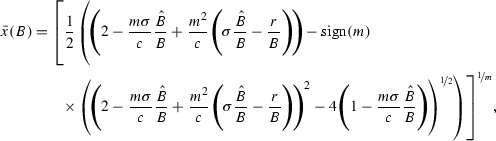
Stationary solution for $s \ge 0, \gamma = 0$ Define the stationary points of this system as $\bar{s}$ and $\bar{q}$ (or equivalently $\bar{x}$).¹³ In Appendix 1.2 it is shown that the unique stationary imitation policy, $\bar{s}$, and the unique interior stationary relative productivity level, $\bar{x} \in (0,x^{*})$, are

$$\begin{aligned} \bar{s} =\frac{B \frac{1}{m}(1 - \bar{q}) - \frac{r}{c}}{\frac{1}{m}(1-\bar{q}) + \bar{q}}, \end{aligned}$$

(37)

(38)

From Assumption 1 and Lemma 1 it follows that $\bar{s}>0$. Thus agents choose strictly positive expenditure on imitation at the stationary point in equilibrium.

In Proposition 1 and Proposition 2 we show that the unique stationary point $(\bar{x},\bar{s})$ is stable. Therefore, paths that converge to $(\bar{x},\bar{s})$ automatically satisfy the transversality condition. Substituting these values into Eq. (26) yields

$$\begin{aligned} \lim _{t \rightarrow \infty } e^{- r t}\lambda (t)x(t) = \lim _{t \rightarrow \infty } e^{- r t}\bar{\lambda }\bar{x} = \frac{1}{r + c \bar{s} \bar{x}^m} \lim _{t \rightarrow \infty } e^{- r t} = 0. \end{aligned}$$

(39)

It remains to show that the agent’s optimization problem satisfies the second order sufficiency conditions. It is sufficient to prove the concavity of the maximized Hamiltonian with respect to $x$ (see Seierstad and Sydsaeter 1977, Theorems 3 and 10). The following parameter restrictions are sufficient to satisfy the second order conditions (see Appendix 4 in Supplementary Material for details).¹⁴

Assumption 3

$m \ge -1$ and $\tfrac{c}{\sigma } < m +2.$

Note that both conditions in Assumption 3 restrict the efficiency of technology diffusion. Concavity may be lost as technology diffusion becomes too easy, with high $c$ or low $m$.

Summary Lemma 1 summarizes the threshold productivity ratio, $x^{*}$, that separates agents into innovators and imitators. As proven in Sect. 4.2.2, for $x > x^{*}$ all agents choose to innovate at the same rate and grow at the same rate. As proven in Sect. 4.2.3, for $x < x^{*}$ all agents exclusively imitate, and stability of the system $\Psi (s(t),q(t))$ implies that there exists a unique steady state productivity ratio, $\bar{x}$, to which all imitating agents converge. Agents below $\bar{x}$ invest in imitation to take advantage of the high efficiency of technology diffusion and catch up to $\bar{x}$. Agents below $x^{*}$ but above $\bar{x}$ endogenously choose to fall back to $\bar{x}$ to reach the optimal trade-off between consumption and investment in imitation, dictated by the strength of the incentive to adopt technology that is governed by the catch-up function. Imitators do not disappear in the limit, nor is there universal convergence to the frontier.¹⁵

5 The dynamic solution

Proposition 1 characterizes the main results of the paper including the existence, uniqueness, and stability of the stationary solution.

Proposition 1

Let Assumptions 1, 2, and 3 hold. For an arbitrary initial distribution $\Phi (0,x)$:

• A: There exists a threshold ratio $x^* = \left( 1-\frac{m\sigma }{c}\right) ^{1/m}$ such that all agents with $x > x^{*}$, including the leader, do only research. They set $s=0,\,\gamma =B-\frac{r}{\sigma }>0$, and grow at the rate $\sigma B-r$. For $x > x^{*}$, the distribution $\Phi (t,x) = \Phi (0,x)$ for all $t$.

• B: All agents with initial conditions $x < x^{*}$ invest only in technology adoption with $s(t) \ge 0$ and $\gamma (t) = 0$. There exists a strictly positive BGP productivity ratio $0 < \bar{x} < x^{*}$ such that all initial productivity ratios $x < x^{*}$ converge to $\bar{x}$.

Proof

See the cases in Sect. 4 and the conditions in Appendix 2.

Denoting the cases where $m>0$ as logistic diffusions and the cases where $m<0$ as Nelson–Phelps diffusions, Fig. 1 provides examples illustrating system dynamics and Proposition 1. The stylized arrows show how convergence might look towards steady state values for $x$. As can be seen in the lower part of the graph, when the marginal productivity of innovation, $\sigma$, is greater than the marginal productivity of imitation, $D(x)$, the agent chooses to invest entirely in innovation, $\gamma$.¹⁶

Fig. 1

Equilibrium convergence and innovation policies

Proposition 2 characterizes the asymptotic dynamics of the distribution of productivities.

Proposition 2

A balanced growth path equilibrium is a growth rate $g = \sigma B - r$, a steady state imitator productivity ratio $\bar{x}$, an innovator threshold $x^{*}$, and an asymptotic distribution $\Phi (\infty ,x)$ such that

• (1) The growth rate of all agents is $\tfrac{\dot{z}}{z} = g = \sigma B - r$, so $\tfrac{\dot{x}}{x} = 0$ for all $x$.

• (2) For arbitrary $\Phi (0,x)$,

  $$\begin{aligned} \Phi (\infty ,x) = {\left\{ \begin{array}{ll} 0 &{}\quad \mathrm{for} \quad 0 \le x < \bar{x}\\ \Phi (0,x^{*}) &{}\quad \mathrm{for} \quad \bar{x}\le x < x^{*}\\ \Phi (0,x) &{}\quad \mathrm{for} \quad x^{*} \le x \le 1.\\ \end{array}\right. } \end{aligned}$$

Proof

See Proposition 1.

Any initial distribution $\Phi (0,x)$ will converge to this unique balanced growth path. In particular, all initial distributions that agree over support $x > x^{*}$ will converge to the same BGP, since all agents initially below $x^{*}$ converge to $\bar{x}$.

This proposition is illustrated in Fig. 2 for an arbitrary initial distribution $\Phi (0,x)$ and the unique BGP distribution $\Phi (\infty ,x)$. The dynamics and asymptotic distribution are independent of the initial frontier $F(0)$. For any initial distribution, the CDF of the upper tail does not change, while a mass of $\Phi (0,x^{*})$ will accumulate at the equilibrium point $\bar{x}$.

Fig. 2

Balanced growth path distribution

One of the main findings of Benhabib and Spiegel (2005) was that for some parameter values in the logistic case, if its distance to the frontier is too large, “the follower will not be able to keep up, growth rates will diverge, and the income ratio of the follower to the leader will go to zero.” This is because there exists a range of productivities such that the flow of technology diffusion for a given investment in imitation is decreasing in the distance to the frontier. Once the investment expenditures in imitation are endogenized, this finding is reversed. Agents optimally invest in technology diffusion such that they converge to a positive BGP productivity ratio, $\bar{x}$, and then grow at the same rate as the leader.

This can be seen directly from our Eq. (15a), which is equivalent to that of Eq. (4.1) in Benhabib and Spiegel (2005), expressed in our current notation. In Benhabib and Spiegel (2005), $\gamma (t)$ and $s(t)$ are treated as constants that can depend on country specific fixed human capital levels, not as choice variables. When $\gamma (t)$ and $s(t)$ are taken as constants, the solution to the law of motion equation, Eq. (4.4) in Benhabib and Spiegel (2005), is:

$$\begin{aligned} \lim _{t\rightarrow \infty }x\left( t\right) = {\left\{ \begin{array}{ll} \left( 1+\frac{m\left( \sigma \gamma -g\right) }{cs}\right) ^{\frac{1}{m}} &{} \quad \text {if} \quad cs-m \left( \sigma \gamma -g\right) >0 \quad \text {or} \quad m<0 \\ \quad \quad \quad \quad 0 &{} \quad \text {if} \quad cs-m\left( \sigma \gamma -g\right) <0 \quad \text {and} \quad m>0. \end{array}\right. } \end{aligned}$$

(40)

When $\gamma (t)$ and $s(t)$ are chosen optimally, the second case of $\bar{x}=0$ is ruled out, as shown in Eq. (38) and Appendix 2.1.

However we will show in Sect. 6 that if we allow the output productivity parameters $B$ to differ across countries and if $m>0$, the ratio of the productivity level of a country to that of the frontier may go to zero if its $B$ is relatively small, i.e., $\lim _{t\rightarrow \infty } x(t)=0$ (see Proposition 3). For similar reasons as in Benhabib and Spiegel (2005), this depends crucially on the curvature of the catch-up function. This can only happen for $m>0$, including the logistic case $m=1$, and may happen even if investment rates are optimally chosen, because the diffusion rates for $m>0$ eventually decrease as the distance to the frontier increases.

5.1 Catch-up, fall-back, and the shadow value of $x(t)$

The Euler equation characterizes the dynamic trade-offs an agent faces. Joint analysis of the Euler equation and the shadow price and shadow value of $x$ provides intuition for the determinants of equilibrium and the catch-up and fall-back forces that lead to the BGP.

From the Euler equation in (18),

$$\begin{aligned} r =\frac{\dot{\lambda }}{\lambda }+\frac{1}{x}+\left( \sigma \gamma +sD(x)-g\right) +sxD^{\prime }(x). \end{aligned}$$

(41)

As usual, the Euler equation states that at each point in time the total benefit of a marginal unit of $x$, represented by sum of the terms on the right, must equal the discount rate. The term $\frac{\dot{\lambda }}{\lambda }$ is the appreciation in the shadow price of $x$ while $\frac{1}{x}$ is the marginal utility of $x$. The terms $\left( \sigma \gamma +sD(x)-g\right)$ represent the marginal product of $x$, both through innovation and through technology diffusion. The final term, $sxD^{\prime }(x)$, tempers the marginal product of $x$ because a higher $x$ reduces the distance to the frontier and therefore the productivity of future imitation. To see this, note that $D^{\prime }(x)<0$. The agents optimally choose $s$ to determine the rate at which they catch-up, or alternatively fall-back. Hence the strength of catch-up or fall-back depends on the magnitude of $sxD^{\prime }(x)$ with $D^{\prime }\left( x\right)$ exerting a negative force on catch-up or, equivalently, a positive force for fall-back. If, however, the agent optimally sets $s=0$, then $D^{\prime }(x)$ has no direct effect on the change.

Recall $\mu (t)$ can be interpreted as the agent’s valuation of its state $x(t)$ at shadow price $\lambda (t)$. The Euler equation at steady state can be arranged as

$$\begin{aligned} \bar{\mu }&= \frac{1}{r-\bar{s}\bar{x}D^{\prime }(\bar{x})} = \frac{1}{r+c\bar{s}\bar{x}^{m}} \le \frac{1}{r}, \end{aligned}$$

(42)

$$\begin{aligned} \bar{\lambda }&= \frac{1}{\bar{x}}\left( \frac{1}{r-\bar{s}\bar{x}D^{\prime }(\bar{x})}\right) . \end{aligned}$$

(43)

Equations (42) and (43) show the role of $\bar{s}\bar{x}D^{\prime }(\bar{x})$ on imitation and innovation in equilibrium. In a region of innovation where $\bar{s}=0$, the discounted value of the utility flow for a marginal unit of $\bar{x}$ per period is the marginal utility $\frac{1}{\bar{x}}$ discounted by $r$. In fact, in the innovation region where $s=0$, logarithmic utility implies that everywhere along the optimal path the marginal utility of an additional unit of $x$ is $\frac{1}{x}$ while its marginal product is constant. This yields the value of the stock $x(t)$ evaluated at the shadow price $\lambda (t)$ as $\mu (t) =\lambda (t)x(t) =\frac{1}{r}$, and $\lambda (t) = \frac{1}{r} \frac{1}{x(t)}$. In the imitation region where $s>0$ the marginal product of $x$ is no longer constant because, as discussed earlier, $D(x)$ is not constant and $D^{\prime }(x) <0$. An increase in the BGP $\bar{x}$ brings the agent closer to the frontier and diminishes the marginal productivity of imitation. This is reflected by the term $\bar{s} \bar{x} D^{\prime }(\bar{x}) < 0$ which augments the effective discount rate that must be applied to the flow of utility. At the BGP productivity ratio in the imitation region the effective discount rate is $r-\bar{s}\bar{x} D^{\prime }(\bar{x})>r$ (see Eq. 42). This captures the negative impact of higher productivity on the endogenously chosen flow of diffusion. This is the active force in the region of imitation below the innovator threshold $x^{*}$ that causes agents close to the threshold to choose to fall-back to $\bar{x}$. These agents let their relative productivity slip in order to benefit from a higher flow of technology diffusion.

6 Heterogeneous agents and scale effects

Thus far, agents in the model have only differed in their initial conditions. However, we know from previous growth research that many theories of growth exhibit scale effects and productivity differences when country size is taken into account. Output is bounded above by $Bz$ and $z$ is always interpreted as per-capita productivity. Thus, one possible interpretation is that $B$ is related to population size or other fixed factors.¹⁷ In such a case, as analyzed in Sect. 6.1, there are scale effects with heterogeneous $B$. If there were no imitation in the model, then all countries would innovate, and the largest country (with the highest B) would grow the fastest. The model would then exhibit strong scale effects and the stationary distribution would collapse such that the leader would grow large and all other countries would disappear in the limit. However, with technology diffusion we still obtain balanced growth path equilibria with non-degenerate stationary distributions. This is because the diffusion of technology from the frontier will have a locomotive effect and pull the followers along. Thus, technology diffusion can act as a counterbalance to scale effects, and their interaction is essential to determining the limiting dynamics of the model.

We should note that even with heterogeneous $B$, the country with the largest $B$ will not necessarily be the leader in the stationary distribution. Furthermore, with heterogeneous $B$, the stationary distribution is not ergodic and initial conditions matter. For example, if a large country like China started with a low productivity level, it may choose to never overtake the US to become the global leader, even if the US is smaller in population. The catch-up gains from technology diffusion can be large enough to prevent the scale effect from dominating the equilibrium stationary distribution.

Additionally, with heterogeneous $B$, the sign of $m$ determines if countries can be left behind. When technology diffusion is efficient, as in the Nelson–Phelps case of $m=-1$, no country, even those with small $B$, will shrink relative to the leader in the limit. However, when technology diffusion is inefficient, countries with $B$ below a threshold can be left behind and shrink in relative productivity in the limit. Analysis and results on heterogeneous $B$ are presented in the next section.

6.1 Stationary solution with heterogeneous $B$

Although the stationary distribution depends on initial conditions, Proposition 3 characterizes properties of potential stationary distributions of BGP equilibria when agents have heterogeneous $B$.

Assume that the agents have idiosyncratic $B$, s.t. $B_{i}>0 \quad \forall i$. Define the $B$ of the frontier agent at time $t$ as $\hat{B}(t) \equiv \left\{ {B_i | z_i(t) = \max _{i'}\left\{ {z_{i'}(t)}\right\} }\right\}$.

Proposition 3

The stationary distribution depends on the initial condition, $z_i(0) \; \forall i$. Given an initial condition, for $m\ne 0$, the following properties hold for the stationary solution, $x^s(B)$:

• (1) Eventually, the frontier agent’s type is constant. That is, there exists a $\hat{t}$ such that for all $t > \hat{t}, \hat{B}(t) = \hat{B}.$

• (2) Given a $\hat{B}$, the stationary equilibrium as a function of $B$ is

  $$\begin{aligned} x^s(B) = {\left\{ \begin{array}{ll} 0 &{} 0 \le B \le \underline{B} \\ \bar{x}(B) &{} \underline{B} < B < \hat{B}\\ \in \bar{x}(\hat{B})\cup [x^*, 1] &{} B = \hat{B}\\ \bar{x}(B) &{} \hat{B} < B < \bar{B},\\ \end{array}\right. } \end{aligned}$$

  where $\bar{x}(B) \in \left( 0, 1 - \frac{m \sigma \frac{\hat{B}}{B}}{c} \right)$, with

  

  (44)
  $$\begin{aligned}&\underline{B} = \max \left\{ {\hat{B} \frac{m \sigma }{c},0}\right\} , \end{aligned}$$

  (45)
  $$\begin{aligned}&\bar{B} = \hat{B} \left( 1-m+\frac{c}{\sigma }\right) +\frac{r (-c+m \sigma )}{\sigma ^2}. \end{aligned}$$

  (46)

• (3) There may exist equilibria where the frontier agent does not have the highest $B$ (i.e., $\hat{B} < \max \left\{ {B_i}\right\}$ and $x^s(B_i) < x^{*}$ for $B_i > \hat{B}$).

• (4) The only agents who choose to innovate are those with $B = \hat{B}$ (i.e., $\gamma (B) > 0 \implies B = \hat{B}$. Alternatively, $x^s(B) \in (x^{*}, 1] \implies B = \hat{B}$).

• (5) If $m < 0$, then agents cannot be left behind (i.e., $\underline{B} = 0$).

• (6) The maximum $B$ of the imitator is always finite (i.e., $\hat{B} < \bar{B} < \infty$).

• (7) If at time zero, $x(\max \left\{ {{B_i}}\right\} ) > x^{*}$, then the agent with the highest $B_i$ eventually becomes the frontier agent.

Proof

See Appendix 3.

The essential points in Proposition 3 are illustrated in Fig. 3. In the stationary equilibrium there is a unique $B$, denoted as $\hat{B}$, at the frontier. Figure 3 graphs the stationary $x^{s}(B)$ for different $B$’s relative to the equilibrium frontier $\hat{B}$. Since all agents with $B\ne \hat{B}$ have $x^{s}(B)<x^{*}$, only agents with $B=\hat{B}$ choose to innovate, and all other agents choose to invest in technology diffusion. Note that this is true even for $B>\hat{B}$, illustrating that the largest B is not always the leader. There is, however, a limit as to how much larger a $B$ can be compared to the frontier $\hat{B}$, given by $\bar{B}$.¹⁸ Figure 3 also depicts the importance of the sign of $m$ in determining whether agents can be left behind. When $m<0$, imitation is very productive, so there is never a region of agents whose productivity goes to zero relative to the frontier agents in the limit. However, when $m>0$ imitation is not very productive, and agents can be left behind. There exists a lower threshold, $\underline{B}$, such that any agent with $B<\underline{B}$ would choose to imitate and would still grow, but would be at such a disadvantage that ultimately it would fall behind in the limit.¹⁹

Fig. 3

Stationary $x$ for heterogeneous $B$ relative to $\hat{B}$

7 Comparative dynamics

Propositions 1 and 2 document that the unique BGP can be characterized by $g,\,x^{*}$, and $\bar{x}$, but how do these equilibrium values depend on fundamental parameters? This section returns to the homogeneous $B$ case to study how the balanced growth path equilibrium changes as parameters modulating the productivity of investment—$\sigma ,\,m$, and $c$—are varied.

7.1 Comparative dynamics for Hicks-neutral technical change

The ratio $\theta \equiv \frac{\sigma }{c}$ is a measure of the relative productivity of innovation to imitation and is an important determinant of the equilibrium. As can be seen by rewriting Eq. (29),

$$\begin{aligned} x^{*} = \left( 1 - m \theta \right) ^{1/m}, \end{aligned}$$

(47)

the threshold for imitation versus innovation depends on the ratio $\theta$ rather than on the levels of $\sigma$ and $c$ independently. This is because $x^*$ is determined by the ratio of instantaneous marginal productivities that are linear in $\sigma$ and $c$, as captured in Eq. (27). This is analogous to the optimal capital to labor ratio in a neoclassical growth model, where a Hicks-neutral technology shock does not alter the optimal relative expenditures. Here, changes in $\sigma$ and $c$ that keep $\theta$ constant may act like a Hicks-neutral technical change, since they keep this measure of relative productivity constant.

However, Eq. (38) shows the lack of neutrality on $\bar{x}$.

(48)

The direct dependence of $\bar{x}$ on $c$ comes from the fall-back incentive. Since $\frac{\partial ^2 D(x;c)}{\partial x \partial c} < 0$, as $c$ increases, the strength of the fall-back incentive, $D'(x;c)$, increases. Hence, a seemingly Hicks-neutral increase in the productivity of growth technologies can change the equilibrium outcome. To see this, fix the ratio $\bar{\theta } = \frac{\bar{\sigma }}{{\bar{c}}}$ and multiply these by a total factor productivity term, $A$: $\sigma = A \bar{\sigma }$ and $c = A \bar{c}$.

Proposition 4

An increase in the TFP of growth technologies

• (1) Does not alter the equilibrium ratio of innovators: $\frac{\mathrm{d}x^{*}}{\mathrm{d}A}=0.$

• (2) Decreases the equilibrium BGP productivity ratio of imitators: $\frac{\mathrm{d}\bar{x}}{\mathrm{d}A} < 0.$

• (3) Increases the equilibrium expenditure on imitation: $\frac{\mathrm{d}\bar{s}}{\mathrm{d}A} > 0.$

Proof

$\frac{\mathrm{d}x^{*}}{\mathrm{d}A} = 0$ follows from the definition of $x^{*}$. For $\frac{\mathrm{d}\bar{x}}{\mathrm{d}A} < 0$ and $\frac{\mathrm{d}\bar{s}}{\mathrm{d}A} > 0$ (see Appendix 5 in Supplementary Material).

A seemingly Hicks-neutral change in the technology level of the economy has no effect on $x^{*}$, but by increasing the strength of the fall-back incentive the change is not neutral in its effect on $\bar{x}$. Even though the growth technology has improved, the growth rate $B \bar{\sigma } A - r$ increases with $A$, so imitators have to increase investment in imitation, $\bar{s}$, to keep up with the higher growth rate. The optimal response is to increase investment some to keep up, but, in response to a better imitation technology, to fall back a bit and benefit from the more efficient flow.

To see how the economy responds to ever increasing TFP in growth technologies take the limit of $A \rightarrow \infty$. Clearly $x^*$ is unchanged. For $\bar{x}$, the terms with a $c$ in Eq. (48) go to zero. Hence,

(49)

Thus $\bar{x}$ decreases as TFP grows, but stays strictly above $0$. This result is in contrast to the comparative dynamics of taking $c$ to $\infty$, where both $x^{*}$ and $\bar{x}$ converge to $1$, as discussed in Sect. 7.4.

Figure 4 provides a numerical simulation of these results for both $m=.5$ and $m=-.5$, demonstrating $\bar{x}(A)$ is decreasing in $A$. In order to better compare the two $m$ values, the figure is normalized by $A=1$.²⁰

Fig. 4

Equilibrium with Hicks-neutral technical change

7.2 Comparative dynamics of $m$

$m$ is a key parameter that affects the efficiency of technology diffusion and distorts imitation incentives depending on the distance to the frontier. The notation $D(x;m)$ is intended to emphasize this dependence.

As discussed in Sect. 4.2.1, the decision of agents to imitate or innovate, summarized by $x^{*}$, depends only on the instantaneous marginal productivity of innovation and imitation (i.e., $D(x;m)$ vs. $\sigma$). A change in $m$ alters the incentives for agents to choose to imitate, as an increase in $m$ decreases the efficiency of technology diffusion. Since $\frac{\partial D(x;m)}{\partial m} < 0$, as $m$ increases, the marginal productivity of imitation decreases.²¹ As imitation becomes less productive, or equivalently as technology diffusion becomes less efficient, more agents will choose to be innovators and there will be less imitators. This is captured in Proposition 5.

Proposition 5

As curvature in the catch-up function changes to make imitation less efficient, the innovator threshold decreases. That is $\frac{\mathrm{d}x^{*}}{\mathrm{d}m} < 0$.

Proof

Taking the derivative of $x^{*}$ from Eq. (29) with respect to $m$ yields

$$\begin{aligned} \tfrac{\mathrm{d}{x^{*}}}{\mathrm{d}{m}} = \frac{\left( 1-\frac{m \sigma }{c}\right) ^{\frac{1}{m}} \left( m \sigma +(c-m \sigma ) \log \left( 1-\frac{m \sigma }{c}\right) \right) }{m^2 (-c+m \sigma )}. \end{aligned}$$

Assumption 2 ensures that $1 - \frac{\sigma m}{c} > 0$, making the denominator negative and the first term of the numerator positive. It remains to show that the second term in the numerator is positive. That is, we need to show

$$\begin{aligned} m \sigma +(c-m \sigma ) \ln \left( 1-\frac{m \sigma }{c}\right) = c \left[ \frac{m \sigma }{c} + \left( 1- \frac{m\sigma }{c} \right) \ln \left( 1-\frac{m \sigma }{c}\right) \right] > 0. \end{aligned}$$

(50)

This term as a function of $\frac{m \sigma }{c}$ achieves a unique global minimum of 0 at $\frac{\sigma m}{c} = 0$.²² Since Assumption 2 restricts $\frac{\sigma m}{c} >0$, this term is strictly positive, and thus $\frac{\mathrm{d}x^{*}}{\mathrm{d}m} < 0$.²³ $\square$

Contrary to $x^{*},\,\bar{x}$ captures the optimal intensity of investment in imitation. An increase in $m$ decreases the instantaneous marginal productivity of imitation, $D(x;m)$, as well as the fall-back incentive, $D'(x;m)$, which will cause agents to adjust their optimal $\bar{x}$ and $\bar{s}$ levels.

Intuitively, decreasing the efficiency of technology diffusion by increasing $m$ also decreases the incentive to fall-back. Formally, $\frac{\mathrm{d}}{\mathrm{d}m}(D'(x;m)) = \frac{\partial ^2 D(x;m)}{\partial x \partial m} = -c x^{-1 + m} \ln (x) > 0$. Since $D'(x;m) < 0$, increasing $m$ lowers the absolute value of $D'(x;m)$ which lowers the fall-back incentive and decreases $\bar{x}$.

Proposition 6

As curvature in the catch-up function changes to make imitation less efficient, the BGP productivity ratio of imitators decreases if $\frac{m}{\bar{q}}\frac{d\bar{q}}{dm}< \ln \bar{q}$. That is $\frac{\mathrm{d}\bar{x}}{\mathrm{d}m} < 0$.

Proof

See Appendix 6.2 (Supplementary Material). In Appendix 6.1 (Supplementary Material), $\frac{\mathrm{d}\bar{q}}{\mathrm{d}m} < 0$ is shown using just Assumptions 1, 2, and 3.

Proposition 7

For the parameter restrictions in Appendix 6.3 (Supplementary Material), as curvature in the catch-up function changes to make imitation less efficient, the BGP level of expenditure on imitation increases. That is $\frac{\mathrm{d}\bar{s}}{\mathrm{d}m} > 0$.

Proof

See Appendix 6.3 (Supplementary Material).

The parameter restrictions in Propositions 6 and 7 are in addition to those in Assumptions 1, 2, and 3. However, in all numerical exercises we have examined, Assumptions 1, 2, and 3 alone have ensured $\frac{\mathrm{d}\bar{x}}{\mathrm{d}m} < 0$ and $\frac{\mathrm{d}\bar{s}}{\mathrm{d}m} > 0$.

Figure 5 illustrates the comparative dynamics of the economy with respect to changes in the efficiency of technology diffusion, $m$. Proposition 5 states that decreasing the efficiency of diffusion causes $x^{*}$ to fall. That is, as technology diffusion becomes less efficient, a larger mass of agents become innovators and fewer choose to be imitators. As Proposition 6 shows, not only are there fewer imitators as $m$ increases, but imitators choose a BGP productivity ratio, $\bar{x}$, that decreases with $m$. With a lower efficiency diffusion process, imitating agents optimally respond by letting the ratio of their productivity to the technology frontier slip lower and they benefit from the higher diffusion rate that comes from falling behind the frontier. Since $\bar{s}$ is increasing in $m$, along a new BGP with less efficient diffusion, imitators increase expenditures that aid technology diffusion, even as they fall further behind the technology frontier.

Fig. 5

Equilibrium indexed by $m$

If we think of the recent trend of globalization and improvements in information technology as a decrease in $m$, this theory suggests that the new BGP would feature fewer innovators and more imitators, with the imitators spending less to increase diffusion and having a relatively higher ratio of productivity to the technology frontier.

7.3 Does less efficient diffusion technology always lower $\bar{x}$?

Proposition 6 shows that as $m$ increases and imitation gets less efficient, the BGP productivity ratio of imitators always decreases. Imitators choose $\bar{x}$ optimally to balance the incentives for catch-up and fall-back. Since $m$ is not the only parameter controlling the efficiency of technology diffusion, do imitating agents always choose to fall-back as imitation becomes less efficient? Equivalently, does there exist a sequence of $D(x)$ functions where imitation becomes strictly less efficient and agents choose to increase $\bar{x}$?

To show that such a non-monotonicity can occur, Fig. 6 conducts a variation of the experiment described in Sect. 7.2. To construct the sequence of $D(x)$, this new experiment will vary $m$ while changing $c$ to keep $x^{*}(m)$ constant. Hence, instead of the constant $\hat{c}$ with the catch-up function $D(x;m,\hat{c})$, the multiplicative term on the catch-up function will be adjusted to $D(x;m,c(m))$. The $c(m)$ function is implicitly defined by $\left( 1 - \frac{m \sigma }{c(m)} \right) ^{m} = x^{*}(\hat{c})$. For all agents in the imitation region, $\frac{\partial D(x;m,c(m))}{\partial m} < 0$ for all $x < x^{*}$, so an increase in $m$ makes imitation less productive. This particular way of changing $c$ and $m$ also has the advantage of keeping $x^{*}$ constant, which isolates the change in economic incentives on the intensive margin.

Fig. 6

Non-monotonicity of $\bar{x}$

Figure 6 compares the results of changing both $c$ and $m$ to those of Sect. 7.2 where only $m$ changes.²⁴ The left column shows results for an experiment where $c$ is held constant at $\hat{c}$ and only $m$ varies—similar to Fig. 5. The top row shows $D(x;m, \hat{c})$ for several values of $m$ and the bottom row shows $\bar{x}(m,\hat{c})$ and $x^{*}(m,\hat{c})$ as a function of $m$. The right column presents the new results, where the top row shows $D(x; m, c(m))$ and the bottom row shows $\bar{x}(m,c(m))$ and $x^{*}(m,c(m))$.

The results show the non-monotonicity of $\bar{x}(m, c(m))$ even while $x^{*}(m,c(m))$ is constant. For $m < 0$, the fall-back incentive dominates and agents choose to decrease $\bar{x}$. For $m>0$, the imitation technology becomes so inefficient that the catch-up incentive dominates and agents choose to increase $\bar{x}$.

7.4 Comparative dynamics of $c$

While both $c$ and $m$ determine the marginal productivity of imitation, $m$ has a distorting effect depending on the distance to the frontier, while $c$ changes the marginal productivity of innovation linearly and uniformly for all $x$.

From Eq. (72) and Proposition 1, it follows that as $c$ grows large, both $\bar{x}$ and $x^{*}$ go to $1$ and the region where imitators fall behind will disappear. For agents below $\bar{x}$, growth rates increase and approach infinity as they approach the frontier. So for large $c$, we expect only the frontier to do research and all other agents to be infinitesimally close to the frontier doing imitation.²⁵

A critical feature of our catch-up specification is that technology diffusion is not instantaneous; the growth of productivity at each instant depends on some measure of the distance to the frontier. The productivities of firms or countries grow incrementally through diffusion from existing superior technologies at a rate that depends on their investment in diffusion. This formulation differs from instantaneous one-shot adoption which allows the implementation of a new technology drawn from the distribution of existing superior technologies, as in Perla and Tonetti (2013) or Lucas and Moll (2013). The limits for large $c$ give us a way to see how a nearly instantaneous jump occurs, albeit here agents jump to the unique frontier rather than jumping to the productivity of another agent in the economy, as in Perla and Tonetti (2013) or Lucas and Moll (2013).

8 Conclusion

In our baseline model, all agents are identical except for their initial levels of productivity and they choose the intensity of their investments to promote growth through imitation and innovation optimally. Innovation is a simple technology with a constant marginal productivity that does not benefit from externalities. Imitation facilitates technology diffusion from the frontier, with the marginal productivity of imitation modeled by a catch-up function that increases with distance to the technology frontier. In equilibrium, agents optimally segment into innovators and imitators and converge to a unique and stable balanced growth path. All innovators grow at the same rate, and therefore the ratio of their productivity to the technology frontier remains unchanged. In the limit, the ratio of every imitator’s productivity to the technology frontier converges to a value that lies below the threshold, where the incentives for catch-up and fall-back are balanced. When agents find their productivities far below the technology frontier, they choose investments to facilitate the diffusion of technology and catch-up to the balanced growth path by growing quickly. If agents are close to or at the frontier, they focus their investments on promoting technological innovation. Agents with relatively high productivity, but not high enough to innovate, optimally fall-back to the balanced growth path of imitators to take advantage of more efficient technology diffusion. By focusing on the portfolio choice of allocating expenditures between imitation and innovation we describe the key forces that provide incentives for imitators to fall-back and converge to a balanced growth path that lies below the technology frontier. When agents with the same productivity differ in their production due to scale effects or factor endowments, there still exists a non-degenerate stationary distribution. Agents of different scale can nevertheless grow at the same rate precisely because technology diffusion acts as a counterbalance to scale effects, allowing growth at the frontier to pull along the followers.

Appendices

Appendix 1: Solving for policy functions

1.1 1.1 Optimal investment in innovation by the leader

The leader must choose optimal investment in innovation by solving

$$\begin{aligned} \tilde{H}=\ln \left( \left( B-\gamma \right) z\right) +\tilde{\lambda } \sigma \gamma z, \end{aligned}$$

(51)

with

$$\begin{aligned} \dot{z}=\sigma \gamma z, \end{aligned}$$

(52)

and

$$\begin{aligned} \dot{\tilde{\lambda }}=-\frac{\partial \tilde{H}}{\partial z}+r\tilde{\lambda } =-z^{-1}+\tilde{\lambda } \left( r-\sigma \gamma \right) . \end{aligned}$$

(53)

Defining $\tilde{\mu } =\tilde{\lambda } z$ gives

$$\begin{aligned} \dot{\tilde{\mu }}=\dot{\tilde{\lambda }}z+\dot{z}\tilde{\lambda } =-1+\tilde{\mu } \left( r-\sigma \gamma \right) +\sigma \gamma \tilde{\mu } =-1+r\tilde{\mu }. \end{aligned}$$

(54)

The solution is

$$\begin{aligned} \tilde{\mu } \left( t \right) =e^{rt}\left( \tilde{\mu } \left( 0\right) -\frac{1}{r} \right) +\frac{1}{r}, \end{aligned}$$

(55)

and the transversality condition,

$$\begin{aligned} \lim _{t\rightarrow \infty }e^{-rt}\tilde{\mu } \left( t \right) =0, \end{aligned}$$

(56)

immediately requires

$$\begin{aligned} \tilde{\mu } \left( t \right) =\frac{1}{r}. \end{aligned}$$

(57)

Maximizing the Hamiltonian with respect to $\gamma$ yields

$$\begin{aligned} \frac{-1}{B-\gamma } + \tilde{\lambda } z\sigma \le 0. \end{aligned}$$

(58)

Using Eq. (57), optimal investment in innovation satisfies

$$\begin{aligned} \gamma \ge B - \frac{r}{\sigma }, \end{aligned}$$

(59)

which holds with equality since $\gamma > 0$ under Assumption 1. Finally, it is straightforward to show that the maximized Hamiltonian is concave, so that this is indeed an optimal solution. See Appendix 4 (Supplementary Material) for details.

1.2 1.2 Optimal investment in imitation

In the region $x < x^{*}$, only imitation will occur, as stated in Lemma 1. To solve for the policy functions of agents in this region it is useful to perform another change of variables, where the relative distance of the agent to the frontier is distorted by the diffusion parameter $m$: $q(t) \equiv x(t)^m$. Using the chain rule:

$$\begin{aligned} \dot{q} = m q \frac{\dot{x}}{x}. \end{aligned}$$

The law of motion for $q$ is obtained using this change of variables together with the law of motion for $x$ (Eq. 15a) when $\gamma = 0$:

$$\begin{aligned} \frac{\dot{q}}{q} = m \left( \frac{c}{m}(1 - q)s - g\right) . \end{aligned}$$

(60)

The first order necessary condition in Eq. (22), with $\gamma = 0$, gives

$$\begin{aligned} \mu = \frac{m}{c (B-s) \left( 1-q\right) }. \end{aligned}$$

(61)

The law of motion for $\mu$ in terms of $q$ is obtained from Eq. (25)

$$\begin{aligned} \dot{\mu } = -1 + \mu (r + c s q). \end{aligned}$$

(62)

Equations (60), (61), and (62) form a system in the variables $\mu ,q,s$. Eliminating $\mu$ via substitution will create a 2x2 system. First, differentiating Eq. (61) provides

$$\begin{aligned} \dot{\mu } = \frac{m \left( (B-s) \dot{q}+(1-q) \dot{s}\right) }{c (1-q)^2 (B-s)^2}. \end{aligned}$$

(63)

Substituting Eqs. (61) and (63) into (62), and rearranging for $\dot{s}$ gives

$$\begin{aligned} \dot{s} = \frac{(B-s) \left( (-1+q) (-B c+m r+c s+c q (B+(-1+m) s))+m \dot{q}\right) }{m (-1+q)}. \end{aligned}$$

(64)

Substituting for $\dot{q}$ from the law of motion in Eq. (60), generates a first order ODE in $s$ and $q$:

$$\begin{aligned} \dot{s} = \frac{(B-s) \left( B c-m r+q (-2 B c+m (-g m+r)+B c q)-c (-1+q)^2 s\right) }{m (-1+q)}. \end{aligned}$$

(65)

Equations (60) and (65) are a system of 2 nonlinear first-order ODEs in $q$ and $s$. Stacking the equations and defining the vector valued function $\Psi$ yields

$$\begin{aligned} \frac{\mathrm{d}}{\mathrm{d}t}\begin{pmatrix} s(t) \\ q(t)\end{pmatrix}&\equiv \Psi (s(t),q(t)) \end{aligned}$$

(66)

$$\begin{aligned}&= \begin{pmatrix} \frac{(B-s(t)) \left( B c-m r+q(t) (-2 B c+m (-g m+r)+B c q(t))-c (-1+q(t))^2 s(t)\right) }{m (-1+q(t))} \\ m q(t) \left( \frac{c}{m}(1 - q(t))s(t) - g\right) \end{pmatrix}.\quad \quad \end{aligned}$$

(67)

To find the stationary solution, evaluate the first order condition in Eq. (61) at the stationary value $\bar{s}$,

$$\begin{aligned} \bar{s} = B - \frac{1}{c/m \bar{\mu }(1 - \bar{q})}. \end{aligned}$$

(68)

Substituting for $\bar{\mu }$ from Eq. (26) and solving for $\bar{s}$ gives

$$\begin{aligned} \bar{s} =\frac{B \frac{1}{m}(1 - \bar{q}) - \frac{r}{c}}{\frac{1}{m}(1-\bar{q}) + \bar{q}}. \end{aligned}$$

(69)

From Assumption 1 and Lemma 1 it follows that $\bar{s}> 0$.²⁶ To determine the stationary solution for $q(t),\,\bar{q}$, substitute this expression into the stationary law of motion in Eq. (60) to find

$$\begin{aligned} \frac{\dot{q}}{q} = 0 = m \left( \frac{c}{m}(1 - \bar{q})\frac{B \frac{1}{m}(1 - \bar{q}) - \frac{r}{c}}{\frac{1}{m}(1-\bar{q}) + \bar{q}} - g\right) . \end{aligned}$$

(70)

Using the known value of $g$, this becomes a quadratic equation in $\bar{q}$:

$$\begin{aligned} \frac{\sigma B-r }{B}&= \left( \frac{\frac{c}{m}\left( 1-\bar{q}\right) -\frac{r}{B}}{1+\bar{q}(m-1)}\right) \left( 1-\bar{q}\right) , \end{aligned}$$

(71)

$$\begin{aligned} 0&= \bar{q}^{2}-\left( 2-\left( \frac{m\sigma }{c}\right) +\frac{m^{2}}{c}\left( \sigma -\frac{r}{B}\right) \right) \bar{q}+\left( 1-\frac{m\sigma }{c}\right) . \end{aligned}$$

(72)

The roots of this quadratic are

(73)

As is proven in Appendix 2.1, the unique interior stationary solution, $\bar{x} \in (0,x^{*})$, is

(74)

Appendix 2: Stability and uniqueness

1.1 2.1 Uniqueness of interior stationary $\bar{x}$

Lemma 2

For any quadratic of form $y^{2} -a y +b$ with roots $y_{1}$ and $y_{2}$, if $a, b > 0$ and $\text {Discriminant}>0$, then both roots are real and positive. Furthermore, $y_{1},y_{2} \notin [\min \{b,1\}, \max \{b,1\} ]$ if $a > 1 + b$.

Proof

The result that roots are real and positive is a standard property of quadratic equations, as $b$ is the product of the roots and $a$ is the sum of the roots. Assume that there exists a root $\hat{y} \in [\min \{b,1\}, \max \{b,1\} ]$. Note that the product of the roots is given by $P(\hat{y}) = \hat{y}(a-\hat{y})$. Since $P(\hat{y})$ is concave, the argmin of $P$ is either $b$ or 1. If we show that $P(b)>b$ and $P(1)>b$, then we have a contradiction. $P(1) = a-1$ and $P(b) = ba -b^{2}$, so $P(1) > b$ if $a > 1 + b$ and $P(b) > b$ if $a>1+b$. Thus if $a > 1 + b,\,\hat{y}$ can not be in $[\min \{b,1\}, \max \{b,1\} ]$.

To show that a unique root $\bar{x} \in (0,x^{*})$ exists, we take Eq. (72) in the form of $\bar{q}^2 - a \bar{q} + b$, where

$$\begin{aligned} a = 2-\left( \frac{m\sigma }{c}\right) +\frac{m^{2}}{c}\left( \sigma -\frac{r}{B}\right) \text{ and } b = 1-\frac{m\sigma }{c}. \end{aligned}$$

$b>0$ from Assumption 2. $a > 0$ using Assumptions 1 and 2. Additionally, the discriminant is positive:

$$\begin{aligned} D&= \left( \left( 2-\left( \frac{m\sigma }{c}\right) +\frac{m^{2}}{c}\left( \sigma -\frac{r}{B}\right) \right) \right) ^{2}-4\left( 1-\frac{m\sigma }{c}\right) >\left( 2-\left( \frac{m\sigma }{c}\right) \right) ^{2}-4\left( 1-\frac{m\sigma }{c}\right) , \nonumber \\ \end{aligned}$$

(75)

$$\begin{aligned}&= 4-4\left( \frac{m\sigma }{c}\right) +\left( \frac{m\sigma }{c}\right) ^{2}-4+4\left( \frac{m\sigma }{c}\right) =\left( \frac{m\sigma }{c}\right) ^{2}\ge 0. \end{aligned}$$

(76)

Thus the $\bar{q}$ roots are real and positive, and hence $\bar{x}$ roots are real and positive. It remains to show that there is a unique $\bar{x} \in (0,x^{*})$. That is, there exists a unique $\bar{q}$ s.t. $\bar{q}^{\frac{1}{m}} < b^{1/m}$. Using Assumption 1, the conditions in Lemma 2 are satisfied, i.e., $a > 1+b$:

$$\begin{aligned} a-(1+b)&= 2-\frac{m \sigma }{c} + \frac{m^{2}}{c}\left( \sigma -\frac{r}{B}\right) -\left( 1+ 1-\frac{m\sigma }{c}\right) ,\nonumber \\&= \frac{m^2}{c}\left( \sigma - \frac{r}{B}\right) >0. \end{aligned}$$

Thus, by Lemma 2, $\bar{q}_{1}, \bar{q}_{2} \notin [\min \{1-\frac{m\sigma }{c},1\}, \max \{1-\frac{m\sigma }{c},1\} ]$. Note for $m>0$, if both roots were less than $1-\frac{m\sigma }{c}<1$ or both roots were greater than one, the product could not be $1-\frac{m\sigma }{c}$. Note for $m<0$, if both roots were greater than $1-\frac{m\sigma }{c}>1$ or both roots were less than one, the product could not be $1-\frac{m\sigma }{c}$. Let convention be that $\bar{q}_{1} < \bar{q}_{2}$. Thus $\bar{q}_{1} < 1-\frac{m\sigma }{c}$ and $\bar{q}_{2} > 1-\frac{m\sigma }{c}$.

Note if $m>0$, then $\bar{x}< (1-\frac{m\sigma }{c})^{1/m}$ iff $\bar{q} < (1-\frac{m\sigma }{c})$ and if $m<0,\,\bar{x}< (1-\frac{m\sigma }{c})^{1/m}$ iff $\bar{q} > (1-\frac{m\sigma }{c})$. Therefore, the smaller root, $\bar{q}_{1}$, is the unique stationary solution if $m>0$ and the larger root, $\bar{q}_{2}$, is the unique stationary solution if $m<0$. Thus there exists a unique root $\bar{x} \in (0,x^{*})$.

1.2 2.2 Stability of BGP

The proof of stability for the entire parameter space is completed as follows: First, prove stability for a particular $r$ by ensuring the determinant of the Jacobian of the dynamic system $\Psi (\cdot ,\cdot ),\,J_{\Psi }(\cdot ,\cdot )$, is negative. Then, use a homotopy argument to show that the system must remain stable as $r$ is varied throughout the rest of the valid parameter space.

Repeating Eq. (36),

$$\begin{aligned} \frac{\mathrm{d}}{\mathrm{d}t}\begin{pmatrix} s \\ q\end{pmatrix} = \Psi (s,q) \equiv \begin{pmatrix} \frac{(B-s) \left( B c-m r+q (-2 B c+m (-\sigma B - r m+r)+B c q)-c (-1+q)^2 s\right) }{m (-1+q)} \\ m q \left( \frac{c}{m}(1 - q)s - \sigma B - r\right) \end{pmatrix}. \end{aligned}$$

Taking the Jacobian of this and simplifying yields

$$\begin{aligned}&J_{\Psi }(s,q)\nonumber \\&\quad = \begin{pmatrix} \frac{-2 B c+m r-q \left( m (1+m) r-B \left( 4 c+m^2 \sigma \right) +2 B c q\right) +2 c (-1+q)^2 s}{m (-1+q)}&{} \frac{(B-s) \left( -m^2 r+B \left( c+m^2 \sigma \right) +B c (-2+q) q-c (-1+q)^2 s\right) }{m (-1+q)^2} \\ -c (-1+q) q &{} m (r-B \sigma )+(c-2 c q) s \end{pmatrix}.\nonumber \\ \end{aligned}$$

(77)

For the starting point of the homotopy argument, take the limit as $r \rightarrow \sigma B$, where $g \rightarrow 0$. As proven in Appendix 2.1, $\bar{q}_1$ is the unique stationary root if $m > 0$, and $\bar{q}_2$ is the unique stationary root if $m < 0$. In either case, the stationary solution, $\Psi (\bar{s},\bar{q})=0$, as $r \rightarrow \sigma B$ is

$$\begin{aligned} \bar{s} = 0,\quad \bar{q} = 1 - \frac{m \sigma }{c}. \end{aligned}$$

(78)

Substituting these into the the Jacobian in Eq. (77) generates

$$\begin{aligned} J_{\Psi }(\bar{s},\bar{q}) =\begin{pmatrix} -B c-(1+m) r+\frac{c r}{\sigma }+B (2+m) \sigma &{} \frac{B c \left( -c r+B c \sigma +B \sigma ^2\right) }{m \sigma ^2}\\ m \sigma \left( 1-\frac{m \sigma }{c}\right) &{} m (r-B \sigma )\\ \end{pmatrix}. \end{aligned}$$

Taking $r \rightarrow \sigma B$ and simplifying further gives

$$\begin{aligned} =\begin{pmatrix} B \sigma &{} (B^2 c)/m\\ m \sigma \left( 1-\frac{m \sigma }{c}\right) &{} 0\\ \end{pmatrix}. \end{aligned}$$

(79)

The determinant of this Jacobian evaluated at the steady state in the limit as $r \rightarrow \sigma B$ is

$$\begin{aligned} \det \left( J_{\bar{\Psi }} \right) \equiv \det \left( J_{\Psi }(\bar{s},\bar{q}) \right) = B^2 \sigma (m \sigma -c). \end{aligned}$$

(80)

The parameter restriction in Assumption 2 ensures that $(m\sigma - c) < 0$, and thus $\det \left( J_{\bar{\Psi }}\right) < 0$. Thus for a small neighborhood around $r = \sigma B$ the system has local saddle-point stability. For clarity of exposition, let $\Gamma (s,x)$ be the equivalent system to $\Psi (s,q)$ in $x$ space. Since $\det \left( J_{\bar{\Psi }}\right) <0$ near $r=B\sigma$, then $\det \left( J_{\bar{\Gamma }}\right) <0$ near $r=B\sigma$.

To complete the proof, use a homotopy argument for varying $r$, by parameterizing the system of equations by $r$: $\Gamma _{r}(s(r),x(r))$. Let $y(r) = (s(r),x(r))$ and the steady state, $\bar{y}(r) =\left( \bar{s}(r), \bar{x}(r) \right)$, be defined by $\bar{\Gamma }_{r} \equiv \Gamma _{r}\left( \bar{y}\right) = 0$ for $r\in S$ where $S=\left\{ \varepsilon ,B\sigma -\varepsilon \right\}$ for any small $\varepsilon >0$. Since $\det \left( J_{\bar{\Gamma }_{r}}\right) <0$ near $r=B\sigma$, it is negative at $r = B \sigma -\varepsilon$ for small $\varepsilon >0$.

Let $\left\{ \bar{y}(r) \right\} =\left\{ \Gamma _{r}^{-1}(0) \right\}$ for isolated zeros of $\Gamma _{r}(\bar{y})$. For $r \in S$ let $\bar{y}(r) \in \mathcal {D}\,\subset (0,B) \times (0,1)$, where $\mathcal {D}$ is chosen so that there are no $\bar{y}(r)\in \partial \mathcal {D}$. Then the homotopy invariant Poincare–Hopf degree on the boundary $\partial \mathcal {D}$ of $\mathcal {D}$ is $\mathop {\displaystyle \sum }_{y \in \left\{ \bar{y}(r) \right\} } \mathrm{sign} \det \left( J_{\Gamma _{r}}(y)\right) = 1$ or $-1$. See Milnor (1965). Since, from Eq. (38), the stationary point $\bar{x}(r)$, and therefore $\bar{y}(r)$, is always unique for $r \in S$, then $\mathrm{sign}\det \left( J_{\Gamma _{r}}(\bar{y}(r) ) \right) =\mathrm{sign} \det J_{\Gamma _{r}}(\bar{y}\left( B\sigma -\varepsilon \right) )=-1$.

If the roots of $J_{\Gamma _{r}}\left( \bar{y}(r) \right)$ are real, then they must be of opposite sign. Therefore $\det \left( J_{\Gamma _{r}}\left( \bar{y}(r) \right) \right) <0$ for $r\in S$ and the system is locally saddle-point stable: given $x(0)$ we can choose $s(0)$ on the stable manifold converging to $\bar{y}\left( r\right)$. Note that the roots of $\det \left( J_{\Gamma _{r}}\left( \bar{y}(r) \right) \right)$ cannot be complex since the determinant, the product of the roots, would have to be positive in that case. Therefore $x$ is a continuous function of time described by the solution of $\dot{x}=\sigma \gamma x+s\left( x\right) x \frac{c}{m}\left( 1- x^{m}\right)$ with $s\left( x\right)$ optimally chosen for $r\in S.$ Therefore the BGP has to be globally stable since $\frac{dx}{dt} \ne 0$ at points other than at the unique $\bar{x}(r)$, or the BGP would not be unique. Thus, it must be that $\frac{dx}{dt}>0$ to the left of $\bar{x}$ and $\frac{dx}{dt}<0$ to the right of $\bar{x}$, so the unique BGP is stable: all agents with productivities $x(t)<x^{*}$ eventually end up at $\bar{x}\left( r\right)$.

Appendix 3: Agents with heterogeneous $B$

Assume that the agents have idiosyncratic $B$, s.t. $B_{i}>0 \quad \forall i$. Define the $B$ of the frontier agent at time $t$ as $\hat{B}(t) \equiv \left\{ {B_i | z_i = \max _{i'}\left\{ {z_{i'}}\right\} }\right\}$. In this Appendix section, we prove Proposition 3.

1.1 3.1 Eventually, the frontier agent’s type is constant

To show that there are no oscillations at the frontier in the stationary equilibrium, assume there was an oscillating set of frontier agents with different values of $B$. Compare pairwise any two values for $B$ within this set. In the instance where the higher $B$ becomes the leader, the first order conditions show that it will continue to innovate at a rate faster than that of a lower B innovator, and thus never fall behind. By process of pairwise iteration through the set of potential frontier agents, the highest $B$ within the set of potential frontier agents must eventually become the leader for all time. Thus, there exists a $\hat{t}$ such that for all $t > \hat{t}, \hat{B}(t) = \hat{B}$. Then, following the solution for the frontier agent in Sect. 3, $g \equiv \hat{B}\sigma - r$ for all $t > \hat{t}$.

To solve for full dynamics, the problem is no longer autonomous, as $g$ depends on the growth rate of the current frontier agent. However, for $t > \hat{t}$ the Hamiltonian for an agent with state $x$ and parameter $B$ is identical to Eq. (16).

1.2 3.2 Regions of innovation and imitation

Following identical algebra to Sect. 4.2.1, the indifference point between innovating and imitating is $x^{*} \equiv \left( 1 - \frac{\sigma m}{c} \right) ^{1/m}$. Hence, the innovation threshold is independent of the particular $B$ of an agent and the $\hat{B}$ of the frontier agent.

1.3 3.3 Innovation only: $x > x^{*}$

Consider the stationary solution where an agent with parameter $B$ innovates forever. The first order condition is identical to Eq. (32). As they innovate forever, the Lagrange multiplier is identical to Eq. (57). Combining these equations yields the optimal policy, $\gamma (B) = B - r/\sigma$. Substituting into the law of motion generates,

$$\begin{aligned} \frac{\dot{x}}{x} = \gamma \sigma - g = \sigma (B - \hat{B}). \end{aligned}$$

(81)

If $B \ne \hat{B},\,x$ cannot be stationary as it grows at a constant rate towards either the frontier or the imitation region. Hence, the only agents in the innovation region of the stationary solution are those with $B = \hat{B}$.

1.4 3.4 Imitation only: $x < x^{*}$

For the stationary solution, the algebra follows identically to Eq. (70). The growth rate of the frontier is $g(\hat{B}) = \sigma \hat{B} - r$. In Eq. (70), define $\hat{\sigma } \equiv \sigma \frac{\hat{B}}{B}$, then Eq. (71) becomes

$$\begin{aligned} \frac{\sigma \hat{B}-r }{B} = \frac{\hat{\sigma } B-r }{B} = \left( \frac{\frac{c}{m}\left( 1-\bar{q}\right) -\frac{r}{B}}{1+\bar{q}(m-1)}\right) \left( 1-\bar{q}\right) . \end{aligned}$$

The derivation is then identical to Appendix 1.2, with the new $\hat{\sigma }(\hat{B})$. This yields the quadratic

$$\begin{aligned} 0&= \bar{q} ^{2} - \left( 2 + \frac{m^{2}}{c}\left( \hat{\sigma } - \frac{r}{B}\right) - \frac{m}{c}\hat{\sigma } \right) \bar{q} + \left( 1 - \frac{m}{c} \hat{\sigma } \right) , \end{aligned}$$

(82)

$$\begin{aligned}&= \bar{q} ^{2} - \left( 2 + \frac{m^{2}}{c}\left( \frac{\hat{B}}{B}\sigma - \frac{r}{B}\right) - \frac{m}{c}\frac{\hat{B}}{B}\sigma \right) \bar{q} + \left( 1 - \frac{m}{c}\frac{\hat{B}}{B}\sigma \right) . \end{aligned}$$

(83)

The solution for the interior root is then $\bar{x}(B)$, where

(84)

(85)

1.5 3.5 Existence of interior $\bar{x}(B) \in \left( 0, 1 - \frac{m \sigma \frac{\hat{B}}{B}}{c} \right)$

Using $\hat{\sigma } = \sigma \frac{\hat{B}}{B}$, by Lemma 2, $\bar{q}_{1},\bar{q}_{2}\notin [\min \{1-\frac{m\sigma \frac{\hat{B}}{B}}{c},1\},\max \{1-\frac{m\sigma \frac{\hat{B}}{B}}{c},1\}]$. Note for $m>0$, if both roots were less than $1-\frac{m\sigma \frac{\hat{B}}{B}}{c}<1$ or both roots were greater than one, the product could not be $1-\frac{m\sigma \frac{\hat{B}}{B}}{c}$. Note for $m<0$, if both roots were greater than $1-\frac{m\sigma \frac{\hat{B}}{B}}{c}>1$ or both roots were less than one, the product could not be $1-\frac{m\sigma \frac{\hat{B}}{B}}{c}$. Let convention be that $\bar{q}_{1}<\bar{q}_{2}$. Thus $\bar{q}_{1}<1-\frac{m\sigma \frac{\hat{B}}{B}}{c}$ and $\bar{q}_{2}>1-\frac{m\sigma \frac{\hat{B}}{B}}{c}$.

Now note that if $m>0$, then $\bar{x}<(1-\frac{m\sigma \frac{\hat{B}}{B}}{c})^{1/m}$ iff $\bar{q}<(1-\frac{m\sigma \frac{\hat{B}}{B}}{c})$ and if $m<0, \bar{x}<(1-\frac{m\sigma \frac{\hat{B}}{B}}{c})^{1/m}$ iff $\bar{q}>(1-\frac{m\sigma \frac{\hat{B}}{B}}{c})$. Therefore, the smaller root, $\bar{q}_{1}$, is the unique stationary solution if $m>0$ and the larger root, $\bar{q}_{2}$, is the unique stationary solution if $m<0$. Thus, there exists a unique root $\bar{x}(B) \in \left( 0,1-\frac{m\sigma \frac{\hat{B}}{B}}{c}\right)$.

We can now derive $\underline{B}$ and $\bar{B}$.

1.6 3.6 Derivation of $\underline{B}$

From Eq. (85), solve for the $B$ such that $\bar{x} = 0$, which determines the lower crossing point. Solving for this root gives,

$$\begin{aligned} \underline{B} = \frac{m \sigma }{c}\hat{B}. \end{aligned}$$

From Assumption 2, $\underline{B} < \hat{B}$, and if the agent has the $B$ of the frontier (i.e., $\hat{B} = B$), then this reduces directly to Assumption 2. Note, if $m<0$, then $\not \exists \; \; B>0 \, \text{ s.t. } \bar{x}=0$.

1.7 3.7 Derivation of $\bar{B}$

From Eq. (85), solve for the $B$ such that $\bar{x} = x^{*}$, which determines the upper crossing point. Solving for this root gives,

$$\begin{aligned} \bar{B} = \hat{B} \left( 1-m+\frac{c}{\sigma }\right) +\frac{r (-c+m \sigma )}{\sigma ^2}. \end{aligned}$$

Rearranging yields

$$\begin{aligned} \frac{\bar{B}}{\hat{B}}&= 1+\frac{c-m\sigma }{\sigma }\left( 1-\frac{r}{\sigma \hat{B}}\right) . \end{aligned}$$

From Assumption 1, which guarantees positive growth at the frontier, $\frac{r}{\sigma \hat{B}}<1$, and from Assumption 2, $c-m\sigma >0$. Thus, $1 < \frac{\bar{B}}{\hat{B}} < \infty$.

Lemma 3

For all $B<\hat{B},\,\bar{x}(B)<x^{*}$.

Proof

Remember that $x^{*}= (1-\frac{m\sigma }{c})^{\frac{1}{m}}$ and $\bar{x}<(1-\frac{m\sigma \frac{\hat{B}}{B}}{c})^{1/m}$. To determine the relationship between $x^{*}$ and $\bar{x}$ there are four cases, $m$ positive or negative and $\frac{\hat{B}}{B}$ above or below one.

If $B<\hat{B}$, for both $m>0$ or $m<0$, then

$$\begin{aligned} x^{*} = \left( 1-\frac{m\sigma }{c}\right) ^{\frac{1}{m}} > \left( 1-\frac{m\sigma }{c}\frac{\hat{B}}{B}\right) ^{\frac{1}{m}}>\bar{x}. \end{aligned}$$

However, if $B>\hat{B}$, for both $m>0$ or $m<0$, either

$$\begin{aligned} \left( 1-\frac{m\sigma }{c}\frac{\hat{B}}{B}\right) ^{\frac{1}{m}}>\bar{x} \ge \left( 1-\frac{m\sigma }{c}\right) ^{\frac{1}{m}}=x^{*} \quad \text{ or } \quad \left( 1-\frac{m\sigma }{c}\frac{\hat{B}}{B}\right) ^{\frac{1}{m}}>\left( 1-\frac{m\sigma }{c}\right) ^{\frac{1}{m}}=x^{*} \ge \bar{x}. \end{aligned}$$

In brief, if $B<\hat{B}$, then $\bar{x}<x^{*}$, but if $B>\hat{B}$ then it is possible but not necessary for $\bar{x}>x^{*}$.

Lemma 4

For all $B<\bar{B},\,\bar{x}(B)<x^{*}.$

Proof

We have shown that given $\hat{B}$ there is a unique $\bar{B}$ such that $\bar{x}=x^{*}$. Now we can show that for $B<\bar{B},\,\bar{x}(B)<x^{*}$. From Lemma 3, for $B<\hat{B},\,\bar{x}(B)<x^{*}$. But there is a unique $\bar{B}>\hat{B}$ at which $\bar{x}(B)=x^{*}$, so by continuity of $\bar{x}$ in $B,\,\bar{x}(B)<x^{*}$ for $B \in (\hat{B},\bar{B})$.

To prove that the solution is stable for $t > t^{*}$, parameterize $r(\tau )$ and $B(\tau )$ to be continuous functions for $\tau \in [0,1]$, where $\tilde{r}(0) = \sigma \hat{B},\,\tilde{r}(1) = r,\,\tilde{B}(0) = \hat{B}$, and $\tilde{B}(1) = B$. Then use the same homotopy argument as in Appendix 2.2, but over $\tau$ instead of $r$. As the set of $(B,r) \in [0, \bar{B}]\times [\sigma B, \infty )$ is connected, any point in the parameter space can be reached by appropriately chosen functions $r(\tau )$ and $B(\tau )$.

Finally, note that for any $B_{1}$ and $B_{2}$ such that $B_{1} < \bar{B}(B_{2})$ and $B_{2} < \bar{B}(B_{1})$, there exist initial conditions leading to stationary solutions, $(\bar{x}(B_{2}), 1)$ and $(1, \bar{x}(B_{1}))$. Hence, given a set of $B$, there are several possible stationary solutions. Now, for each of these initial conditions, perturb an $\epsilon$ such that $(\bar{x}(B_{2}) + \epsilon , 1)$ and $(1, \bar{x}(B_{1}) + \epsilon )$. Since $\bar{x}(B) < x^{*}$ and the solutions are stable, these perturbed initial conditions will approach the respective stationary solutions. Hence, the system is not ergodic, and the stationary solution depends on the initial conditions.

1.8 3.8 Non-existence of innovators with $B \ne \hat{B}$

By contradiction, separately consider the cases where $B > \hat{B}$ and $B < \hat{B}$.

Assume that there exists a $B$ such that $B > \hat{B}$ with a stationary $x^{*} \le x^s(B) < 1$. From Eq. (81), if the agent is an innovator and $B > \hat{B}$, then $x(t)$ has a constant, positive growth rate and hence is not stationary (i.e., will eventually overtake the existing $\hat{B}$ frontier).

Alternatively, assume that there exists a $B < \hat{B}$ such that $x^{*} \le x^s(B) < 1$. From Eq. (81), if the agent is an innovator, then $x(t)$ has a constant, negative growth rate and is not stationary (i.e., will eventually drop to $x(t) \le x^{*}$, and hence enter the imitation region).

1.9 3.9 Non-existence of equilibria with imitators $B>\bar{B}$

We want to show that there does not exist an equilibrium in which agents with $B>\bar{B}$ imitates. There are two possible cases: the agent invests only in imitation or the agent invests in some combination of imitation and innovation.

For case one, assume by contradiction that an equilibrium exists in which an agent with arbitrarily large $B/\hat{B}$ invests only in imitation. As proved in the derivation of $\bar{B} > \hat{B}$, since $\bar{x}(B)$ crosses $x^{*}$ at $\bar{B}$, any agent with $B > \bar{B}> \hat{B}$ would optimally choose to invest in innovation, contradicting that it optimally invests only in imitation.

For case two, assume there exists a stationary equilibrium such that $B > \hat{B}$ and the agent invests in both innovation and imitation simultaneously. By using the two first-order necessary conditions in Eq. (27), this is only possible if $x^s(B) = x^{*}$, where the agent optimally remains at the $x^{*}$ threshold. Next, note that from the first order condition, $\sigma = D(x^{*})$, so the law of motion is

$$\begin{aligned} 0 = \frac{\dot{x}}{x} = \sigma \bar{\gamma } + D(x)\bar{s} - \sigma \hat{B} + r = \sigma (\bar{\gamma } + \bar{s}) - \sigma \hat{B} + r. \end{aligned}$$

Since the returns to innovation and imitation are identical at $x^{*}$, the optimal investment composition between innovation and imitation is indeterminate. Nonetheless, total investment is $\bar{\gamma } + \bar{s} = \hat{B} - \frac{r}{\sigma }$.

Rephrasing the contradiction, assume that for some $B > \hat{B}$, the choice of $x^s(B) = x^{*}$ and $\bar{\gamma } + \bar{s} = \hat{B} - \frac{r}{\sigma }$ is the optimal solution. Then the optimal path of $z$ is $z(t) = z_0 e^{g(\hat{B}) t}$, where $z_0$ is an initial condition and $g(\hat{B}) \equiv \sigma \hat{B} - r$. Substituting into the agent’s optimization problem in Eq. (1) yields,

$$\begin{aligned} U(z;B, \hat{B})&= \int \limits _{0}^{\infty }\left( \ln \left( Bz-sz-\gamma z\right) \right) e^{-rt}dt, \end{aligned}$$

(86)

$$\begin{aligned}&= \int \limits _{0}^{\infty }\left( \ln (z_0 e^{g(\hat{B}) t}) + \ln \left( B-\hat{B} + \frac{r}{\sigma }\right) \right) e^{-rt}dt,\end{aligned}$$

(87)

$$\begin{aligned}&= \left( \ln (z_0) + \frac{1}{m}\ln \left( 1 - \frac{\sigma m }{c}\right) + \ln \left( B-\hat{B} + \frac{r}{\sigma }\right) \right) \int \limits _{0}^{\infty }e^{-rt}dt\nonumber \\&\quad + \left( \sigma \hat{B} - r \right) \int \limits _{0}^{\infty }t e^{-rt}dt,\end{aligned}$$

(88)

$$\begin{aligned}&= \frac{1}{r}\ln (z_0) + \frac{1}{r}\ln \left( B-\hat{B} + \frac{r}{\sigma }\right) + \frac{1}{r^2}\left( \sigma \hat{B} - r \right) . \end{aligned}$$

(89)

An alternative feasible policy would be for this agent to choose to become the frontier agent and grow at a rate $g = \sigma B - r$. In that case $z(t) = z_0 e^{g(B) t}$ and the value is

$$\begin{aligned} U(z;B, B)&= \int \limits _{0}^{\infty }\left( \ln (z_0 e^{(\sigma B - r) t}) + \ln \left( \frac{r}{\sigma }\right) \right) e^{-rt}dt, \end{aligned}$$

(90)

$$\begin{aligned}&= \frac{1}{r}\ln (z_0) + \frac{1}{r}\ln \left( \frac{r}{\sigma }\right) + \frac{1}{r^2}\left( \sigma B - r \right) . \end{aligned}$$

(91)

Comparing the value of the two policies by subtracting Eq. (89) from Eq. (91),

$$\begin{aligned} U(z;B, B) - U(z;B, \hat{B}) = \frac{1}{r}\left( \frac{\sigma }{r}(B - \hat{B})-\ln \left( \frac{\sigma }{r}(B - \hat{B}) + 1 \right) \right) . \end{aligned}$$

(92)

Since $B - \hat{B}>0$,

$$\begin{aligned} U(z;B, B) - U(z;B, \hat{B}) \ge 0. \end{aligned}$$

(93)

This expression holds with equality iff $B = \hat{B}$. Therefore, we have a contradiction as the choice to become the frontier agent dominates the policy of investing in innovation and imitation simultaneously to remain at $x^{*}$ with leader $\hat{B}$.

References

Acemoglu, D., Aghion, P., & Zilibotti, F. (2006). Distance to frontier, selection and economic growth. Journal of the European Economic Association, 4(1), 37–74.
Acemoglu, D., Robinson, J. A., & Verdier, T. (2012). Can’t we all be more like Scandinavians? Asymmetric growth and institutions in an interdependent world. NBER Working Paper No. 18441.
Aghion, P., Harris, C., Howitt, P., & Vickers, J. (2001). Competition, imitation and growth with step-by-step innovation. Review of Economic Studies, 68, 467–492.
Aghion, P., & Howitt, P. (1998). Endogenous growth theory. Cambridge, MA: MIT Press.
Aghion, P., & Howitt, P. (2009). The economics of growth. Cambridge, MA: MIT Press.
Aghion, P., Howitt, P., & Mayer-Foulkes, D. (2005). The effect of financial development on convergence: Theory and evidence. The Quarterly Journal of Economics, 120, 173–222.
Alvarez, F., Buera, F., & Lucas, R. E. (2012). Idea flows, economic growth, and trade. New York: mimeo.
Barro, R. J., & Sala-i-Martin, X. (1997). Technological diffusion, convergence, and growth. Journal of Economic Growth, 2(1), 1–26.
Benhabib, J., & Spiegel, M. M. (1994). The role of human capital in economic development: Evidence from aggregate cross-country data. Journal of Monetary Economics, 34(2), 143–173.
Benhabib, J., & Spiegel, M. M. (2005). Human capital and technology diffusion. In P. Aghion & S. Durlauf (Eds.), Handbook of economic growth, chap. 13 (Vol. 1, pp. 935–966). Amsterdam: Elsevier.
Damsgaard, E. F., & Krusell, P. (2010). The world distribution of productivity: Country TFP choice in a Nelson–Phelps economy. NBER Working Paper No. w16375.
Eeckhout, J., & Jovanovic, B. (2002). Knowledge spillovers and inequality. American Economic Review, 92(5), 1290–1307.
Ericson, R., & Pakes, A. (1995). Markov-perfect industry dynamics: A framework for empirical work. The Review of Economic Studies, 62(1), 53–82.
Gerschenkron, A. (1962). Economic backwardness in historical perspective. Cambridge, MA: Belknap Press of Harvard University Press.
Gill, I. S., & Raiser, M. (2012). Golden growth: Restoring the lustre of the European economic model. Washington, DC: The World Bank.
Grossman, G. M., & Helpman, E. (1991). Quality ladders in the theory of growth. The Review of Economic Studies, 58(1), 43–61.
Howitt, P., & Mayer-Foulkes, D. (2005). R &D, implementation, and stagnation: A Schumpeterian theory of convergence clubs. Journal of Money, Credit and Banking, 37(1), 147–177.
Jones, C. I. (2005). Growth and ideas. In P. Aghion & S. Durlauf (Eds.), Handbook of economic growth, chap. 16 (Vol. 1, pp. 1063–1111). Amsterdam: Elsevier.
Jovanovic, B., & Rob, R. (1989). The growth and diffusion of knowledge. Review of Economic Studies, 56(4), 569–582.
Klenow, P. J., & Rodriguez-Clare, A. (2005). Externalities and growth. In P. Aghion & S. Durlauf (Eds.), Handbook of economic growth, chap. 11 (pp. 817–861). Amsterdam: Elsevier.
König, M., Lorenz, J., Zilibotti, F. (2012). Innovation vs imitation and the evolution of productivity distributions. CEPR Discussion Paper No. 8843.
Kortum, S. S. (1997). Research, patenting, and technological change. Econometrica, 65(6), 1389–1420.
Laincz, C. A. (2009). R &D subsidies in a model of growth with dynamic market structure. Journal of Evolutionary Economic, 19, 643–673.
Lucas, R. E. (2009). Trade and the diffusion of the industrial revolution. American Economic Journal: Macroeconomics, 1(1), 1–25.
Lucas, R. E., & Moll, B. (2013). Knowledge growth and the allocation of time. Journal of Political Economy (forthcoming).
Luttmer, E. G. J. (2011). Technology diffusion and growth. Journal of Economic Theory, 147(2), 602–622.
Magaziner, I., & Patinkin, M. (1990). The silent war. New York: Vintage Books.
Milnor, J. W. (1965). Topology from the differentiable viewpoint. Charlottesville, VA: The University Press of Virginia.
Mukoyama, T. (2003). Innovation, imitation, and growth with cumulative technology. Journal of Monetary Economics, 50(2), 361–380.
Nelson, R. R., & Phelps, E. S. (1966). Investment in humans, technological diffusion, and economic growth. American Economic Review, 56(1/2), 69–75.
Parente, S. L., & Prescott, E. C. (1994). Barriers to technology adoption and development. Journal of Political Economy, 102(2), 298–321.
Perla, J., & Tonetti, C. (2013). Equilibrium imitation and growth. Journal of Political Economy (forthcoming).
Rustichini, A., & Schmitz, J. A. (1991). Research and imitation in long-run growth. Journal of Monetary Economics, 27(2), 271–292.
Segerstrom, P. S. (1991). Innovation, imitation, and economic growth. Journal of Political Economy, 99(4), 807–827.
Seierstad, A., & Sydsaeter, K. (1977). Sufficient conditions in optimal control theory. International Economic Review, 18(2), 367–391.
Thompson, P. (2001). The microeconomics of an R &D-based model of endogenous growth. Journal of Economic Growth, 6(4), 263–283.
Thompson, P., & Waldo, D. (1994). Growth and trustified capitalism. Journal of Monetary Economics, 34(3), 445–462.
Acknowledgments
We would like to thank Boyan Jovanovic and Tom Sargent for useful feedback.
Author information
Authors and Affiliations
Corresponding author
Electronic supplementary material
Below is the link to the electronic supplementary material.