
Abstract
Trading systems are tools to aid financial analysts in the investment process in companies. This process is highly complex because a big number of variables take part in it. Furthermore, huge sets of data must be taken into account to perform a grounded investment, making the process even more complicated. In this paper we present a real trading system that has been developed using semantic technologies. These cutting-edge technologies are very useful in this context because they enable the definition of schemes that can be used for storing financial information, which, in turn, can be easily accessed and queried. Additionally, the inference capabilities of the existing reasoning engines enable the generation of a set of rules supporting this investment analysis process.
1 Introduction
Predicting stock market movements is the long cherished desire of investors, speculators, and industries (Kim 2004). According to (Wen et al. 2010), the study of the stock market is a hot topic, because if successful, the result will transfer to fruitful rewards. Moreover, Qian and Rasheed (2006) argue that stock market prediction is attractive and challenging, although this market is extremely hard to model with any reasonable accuracy (Wang 2003). Stock market fluctuations are also the result of complex phenomena (Sitte and Sitte 2002). However, despite this complexity, many factors, including macroeconomic variables and stock market analysis, have been proven to have a certain level of forecast capability in the stock market during a certain period of time (Lo et al. 2000). Stock market research encapsulates two elemental trading philosophies: fundamental and technical approaches (Schumaker and Chen 2009). This paper focuses on the first one. In fundamental analysis, stock market price movements are believed to be derived from earnings, ratios, and management effectiveness to determine future forecasts. In other words, the price of a security can be determined through the nuts and bolts of financial numbers (Schumaker and Chen 2009).
According to Yoda (1994), investment analysis tools can be classified into mechanical tools. Mechanical tools include traditional tools by technical analysis, fundamental analysis and other expanded tools from these two types of analysis. Intelligent tools are the mechanisms which apply intelligent techniques to solve problems, where soft computing is the major representative (Chen and Liao 2007). Having this taxonomy in mind, mixing both investment tools can be seen as an interesting field of study, particularly by building a solution capable of making recommendations on the basis of fundamental analysis and improving these recommendations by means of combining a set of technologies. Following this research trend, we present in this paper FAST (Fundamental Analysis System for Trading): a tool designed to aid investors in the investment process helping to take the most appropriate decision (buy, sell or maintain the share values) in a long term investment.
The remainder of the paper is structured as follows. Section 2 reviews the relevant literature. Section 3 discusses the main features of FAST. Section 4 describes the evaluation of the tool’s performance including a description of the sample, the method, results and discussion. Finally, the paper ends with a discussion of research findings, limitations and concluding remarks.
2 Background
Stock market prediction is attractive and challenging, but also a very difficult issue (Qian and Rasheed 2006). Along with the development of artificial intelligence, more and more researchers try to build automatic decision-making systems to predict the stock market (Kovalerchuk and Vityaev 2000). Thus, soft computing is progressively gaining presence in the financial world (Mochón et al. 2008). Soft computing techniques such as fuzzy logic, neural networks, and probabilistic reasoning draw most attention because of their abilities to handle uncertainty and noise in the stock market (Vanstone and Tan 2005). The main reasons for their popularity include the ability of neural networks to ‘learn’ from the past and produce a generalized model to forecast future prices, freedom to incorporate fundamental and technical analysis into a forecasting model and the ability to adapt according to market conditions (Majhi et al. 2009). Their approach basically employs case-based reasoning approach, i.e., it tries to find a similar case from the past to a given situation (Lee et al. 2010).
Recently, in the first decade of the 21st century, various studies using Artificial Neural Networks (ANN) have been developed in the fields of forecasting stock indexes (e.g. Chavarnakul and Enke 2008; Majhi et al. 2009). Most of the work is the combination of soft computing technology and technical analysis in stock analysis (Wen et al. 2010; Chen et al. 2009; Fernandez Garcia et al. 2010). Although technical analysis is the most popular area of research, fundamental analysis is mostly for long-term investment decision (Quah 2009), due to the fact that most fundamental variables are available in a monthly or annual basis (Anastasakis and Mort 2009). However, as reported in (Quah 2009) it is feasible to complement fundamental and technical analysis in an expert system. In the work of Vanstone and Finnie (Vanstone and Finnie 2009), a deep literature review about the applications of ANN to both fundamental and technical analysis can be found. One of the recent and promising works devoted to the use of fundamental analysis is the work by Quah (2009), in this work, author suggest the use soft-computing models which focus on applying fundamental analysis for equities screening.
Concerning semantic technologies, in the last few years, several finance-related ontologies have been developed. The ontology TOVE (Toronto Virtual Enterprise) (Fox et al. 1998), developed by the Enterprise Integration Laboratory from the Toronto University, describes a standard organization company as their processes. BORO (Business Object Reference Ontology) ontology is intended to be suitable as a basis for facilitating, among other things, the semantic interoperability of enterprises’ operational systems (Partridge and Stefanova 2001). The DIP (Data Information and Process Integration) consortium developed an ontology for the financial domain which was mainly focused to describe semantic web services in the stock market domain (Losada et al. 2005). The eXtensible Business Reporting Language (XBRL) Ontology Specification Group developed a set of ontologies for describing financial and economical data in Resource Description Framework (RDF) for sharing and interchanging data. This ontology is becoming an open standard means of electronically communicating information among businesses, banks, and regulators (XBRL International 2009).
However, the approach of this work is quite different. In the FAST system, semantic technologies are applied with two objectives: in the first place, semantic technologies are used with the objective of defining and using a financial ontology where several financial data will be stored. This storage is used with the intention of reusing the ontology in future systems and of knowledge sharing. The second objective is the application of the inference capabilities that semantic technologies offer.
3 FAST: Calculations, internals and architecture
FAST is based on semantic technologies. Taking full advantage of these technologies, FAST allows the generation of investments for a set of companies, using some financial information stored in an ontology format. The development of the system is based in the reutilization and the improvement of SONAR (Gomez et al. 2009) bringing a complementary approach to CAST (Rodríguez-González et al. 2011). Therefore, the ontology developed in SONAR has been used for the storage of the financial information necessary to execute part of the system. SONAR is also present given that new knowledge is provided by this system and for hence, new financial information is provided by SONAR. However, the purpose of that ontology was not only to save the minimum information required for the inference of the system, but also to save a lot of other financial information (e.g. older share values, news about the company…), which is not required in FAST.
FAST is based in the use of concrete financial data, which is stored in a repository, in order to make long term predictions for a concrete company in a concrete market (Markowitz 1952; Roy 1952; Sharpe 1966; Mullins 1982). Figure 1 shows the main architecture of the FAST system and the connections among their components.

System architecture
The workflow of the system is as follows. The user queries the system asking for an investment recommendation about a certain company (e.g. company X). Once the query has been received, FAST loads all the rules that must be checked in order to provide that recommendation. The rule system asks the Financial Data Reader for the necessary data to execute each rule. The Financial Data Reader module queries the financial ontology to retrieve that information and return back to the Rule Manager. Once the information has arrived to the Rule Manager, it will make interchange calls with the Financial Calculator module that is in charge of executing some financial operations needed, depending on the rule to be executed. The Financial Calculator will write the financial reasoning ontology with all the information generated by each rule. Finally, this ontology will be sent to the selected reasoner (Reasoners module), together with the knowledge base that contains the Semantic Web Rule Language (SWRL) (Horrocks et al. 2004) rules, in order to proceed to make the inference. The result of that inference will be processed and returned to the user in an investment answer format. In what follows the main components and features of FAST are depicted.
3.1 Financial ontology
The main goal of this ontology is to manage the vast amount of existing financial data. The management of this data has been coming into increasingly sharp focus for some time. The financial domain is becoming a knowledge intensive domain, where a huge number of businesses and companies hinge on, with a tremendous economic impact in our society (Gomez et al. 2009). Consequently, there is a need for more accurate and powerful strategies for financial data management.
Semantic technologies are currently achieving a certain degree of maturity. They provide a consistent and reliable basis to face the aforementioned challenges aiming at a fine-grained approach for organization, manipulation and visualization of financial data (Castells et al. 2004).
The language used for the knowledge representation in the financial ontology is Ontology Web Language (OWL) (McGuinness and Harmelen 2004). OWL is the de facto Semantic Web standard language for authoring ontologies. The OWL language provides three increasingly expressive sublanguages: OWL Lite, OWL DL, and OWL Full. Using these languages, ontology authors can create classes, properties and define instances and their operations.
For the purposes of this use case scenario, authors evolved the financial ontology produced in SONAR (Gomez et al. 2009) using OWL DL. In Table 1, some metrics concerning this new financial ontology are presented.
The ontology covers four main financial concepts:
-
A financial market is a mechanism that allows people to easily buy and sell financial assets such as stocks, commodities, currencies, etc. The main stock markets such as Nasdaq, London Stock Exchange or Madrid Stock Exchange have been modeled in the ontology as subclasses of the Stock_Market class.
-
The concept Financial Intermediary represents, among other things, the entities that typically invest on the financial markets. Examples of such entities are banks, insurance companies, brokers and financial advisers.
-
The Asset class represents everything of value on which an Intermediary can invest, such as stock market indexes, commodities, companies, currencies, etc. So, for instance, enterprises such as General Electric or Microsoft belong to the Company concept and currencies such as US dollar or Euro are included as individuals of Currency concept.
-
The Legislation concept comprises the entities that are in charge of supervising the stock market (e.g. the Federal Reserve or the International Monetary Fund), and the regulation and laws that can be applied to the financial domain.
Figure 2 shows an excerpt of the ontology. The ontology is depicted through a Protégé-based graphical notation.

Excerpt of the financial ontology
3.2 Financial data reader
This is the module in charge for retrieving all the financial information needed for each rule. When a rule is selected and executed, part of the execution process consist in retrieving some financial information from the financial ontology, which is accomplished by the financial data reader. In fact, this connection is not established directly with the ontology. Instead, it is made against a SESAME repository which contains the ontology dumped (Broekstra et al. 2002). The idea of using that repository instead of the ontology directly is only because of efficiency. Given the vast amount of data that the other part of the SONAR system deals with (refers to the ontology population tool–not mentioned here because is not related with this work), it is necessary to use a repository that stores all financial information in a database instead of a single OWL file. With the use of the repository the efficiency of the system accessing the data is dramatically increased.
The financial information retrieved by the system will be returned to the rules module in order to be processed. The information that is managed by this module consists in a set of numerical variables which contains financial information like stock values, net incomes, number of shares of a concrete company, etc.
3.3 Financial calculator
This module is in charge of performing the calculations needed for each rule of the system. In what follows, all the concepts used and an explanation for each value is provided. The sub-sections will describe each rule and the formulae used (with the mentioned concepts). Some of the concepts are in the system and therefore do not need to be calculated from others.
It is important to remark that once a value is calculated, it is saved and there is no need to calculate it again. For this reason, in each rule there are concepts such as, for example, Market Capitalization, that are used in more than one rule, but the formula of its calculi is only shown the first time it appears.
The concepts represented by a function (for example: Customers(N)) represent the customers in the “N” th year. If the value is “0”, it represents the actual year, if it is “1”, it represents the previous year to the actual year, and so on.
Financial concepts used:
-
Market capitalization: Measurement of the size of a business enterprise (corporation), which equals the share price times the number of shares of a public company.
-
Number of shares: Represents the total number of shares of the company.
-
Share Value: Represents the current share value of the company.
-
Price to Earnings Ratio (PER): The P/E ratio (price-to-earnings ratio) of a share (also known as “P/E”, “PER”, “earnings multiple”, or simply “multiple”) is a measure of the price paid for a share relative to the annual net income or profit earned by the firm per share.
-
Capital Stock: Total amount of a firm’s capital, represented by the value of its issued common and preferred stock (ordinary and preference shares).
-
Reserves: Part of retained set aside for a specified purpose and, hence, unavailable for disbursements dividends.
-
Cash flow: Cash flow refers to the movement of cash into or out of a business, a project, or a financial product. It is usually measured during a specified, finite period of time.
-
Profit for Period: Profit (or loss) for period after preferred dividends and all other operating and non-operating expenses, but before ordinary dividends distribution.
-
Dividends: Are payments made by a corporation to its shareholder members.
-
EBIT (Earnings before interest and taxes): It is a measure of a firm’s profitability that excludes interest and income tax expenses.
-
Taxes: A fee charged (“levied”) by a government on a product, income, or activity.
-
Amortization: The sum of the process of allocating the cost of depreciation, amortization and depletion expenses.
-
Fixed asset: It is a term used in accounting for assets and property which cannot easily be converted into cash.
-
Investment in operational needs funding (ONF Investment): Investment in Cash and other items required to cover operating expenses.
-
Cash & Cash equivalent: Are the most liquid assets found within the asset portion of a company’s balance sheet.
-
Debtor: An individual or company that owes debt to another individual or company.
-
Stocks: Merchandise bought for resale, and materials and supplies purchased for manufacture for use in revenue production, less any allowances.
-
Creditors: It is a person or institution to which money is owed.
-
Book Value (BV): Book value or carrying value is the value of the company according to its balance sheet account balance.
-
Price to Book (PTB): The price-to-book ratio, or P/B ratio, is a financial ratio used to compare a company’s book value to its current market price.
-
Price Cash Flow Ratio (PCFR): The price/cash flow ratio (also called price-to-cash flow ratio or P/CF), is a ratio used to compare a company’s market value to its cash flow.
-
Total liabilities & Debt: Total amount owned to a person or organization for funds borrowed.
-
Financial expenses: Total periodic expense for using borrowed short and long-term money. In certain countries this also includes debt discounts and foreign exchange losses.
-
Cost of debt: The effective rate that a company pays on its current debt.
-
Total Shareholders’ funds & Liabilities: Includes total liabilities and debt and shareholders’ equity.
-
Equity ratio: The equity ratio is a financial ratio indicating the relative proportion of equity to all used to finance a company’s assets.
-
Interest rate on 5 year Spanish government bond: Interest paid in regular intervals by the Spanish government for purchasing a 5 years bond.
-
Inflation rate: The inflation rate is a measure of inflation, the rate of increase of a price index (for example, a consumer price index).
-
BETA: The beta of a stock is a number describing the relation of its returns with that of the financial market as a whole.
-
Market average return (5 years): The gain or loss of an investment on the whole market over a specified period (5 years), expressed as a percentage increase over the initial investment cost.
-
Cost of equity: The cost of equity is the minimum rate of return a firm must offer shareholders to compensate for waiting for their returns, and for bearing some risk.
-
Discount rate: Is the rate that a company is expected to pay on average to all its security holders to finance its assets.
-
Tax rate: In a tax system and in economics, the tax rate describes the burden ratio (usually expressed as a percentage) at which a business or person is taxed.
-
Growth rate of cash flow: The amount of increase that the cash flow has gained within a specific period.
-
Projected cash flow: Expected cash flow in a specific period.
-
Growth rate of projected cash flow: The amount of increase that the projected cash flow has gained within a specific period.
Next, the rules which have been designed for the correct behavior of the system are explained. Each rule can be divided in a set of rules (or premises) which can be codified and explained separately.
3.3.1 Medium term prediction rule
As is explained in 3.7 section, each rule is divided in some sub rules (that are part of the premises and conclusions of the super rule). In the medium term predictions, are two main rules:
-
PTB Rule:
In this rule is necessary to calculate two main values: PER (Abarbanell and Bushee 1997) and PTB. The calculi done by the system are the following:
In first place, Market capitalization is calculated:
$$ Market\;Capitalization = Number\;of\;shares*Share\;value $$(1)Once the Market capitalization is calculated, we are able to calculate the PER:
$$ PER = Market\;Capitalization/Profit\;for\;Period $$(2)The next value that needs to be calculated is the once called BV, with the following formula:
$$ BV = Capital + Reserves + Profit\;for\;Period - Dividends $$(3)After that, we can calculate PTB:
$$ PTB = Market\;Capitalization/BV $$(4)
-
PCFR Rule:
In this rule is necessary to calculate one value: PCFR (Abarbanell and Bushee 1997). The calculi done by the system are the following:
In first place, ONF Investment is calculated:
$$ \begin{gathered} ONF\;Investment \hfill \\ \begin{array}{*{20}{c}} {\quad \quad \quad \quad \quad \quad = \left( {CCE(0) + Customers(0) + Inventory(0) - Creditors(0)} \right)} \hfill \\ {\quad \quad \quad \quad \quad \quad - \left( {CCE(1) + Customers(1) + Inventory(1) - Creditors(1)} \right)} \hfill \\ \end{array} \hfill \\ \end{gathered} $$(5)Once the ONF Investment is calculated, we calculate the Cash Flow:
$$ Cash\;Flow = EBIT - Taxes + Amortizations - Fixed\;Asset - ONF\;Investment $$(6)Once the Cash Flow is calculated, we are able to calculate the PCFR:
$$ PCFR = Market\;Capitalization/Cash\;Flow $$(7)
3.3.2 Long term prediction rule
The Long Term Prediction Rule has three sub rules. Each rule will fire an investment action (buy, sell or maintain). In this case, one single value is needed to be calculated for the fire of these rules. This rule implies a lot of financial calculus.
In first place, cost of debt is calculated:
After that, equity ratio is calculated:
Next calculus corresponds to cost of equity:
In fourth place, the discount rate is calculated:
In fifth place, Growth rate of cash flow is calculated:
After here, some of the financial values that have been explained before (with their respective description) have been calculated. Now, it is necessary to calculate two interval values that will allow the system to make the investment prediction.
The first one is the value called “first interval”:
After that, we need to calculate some other values. The first one will be the projected cash flow:
Next value will be the growth rate of projected cash flow:
Now, second interval is calculated:
Finally, the last value that will be calculated and that will return the investment signal is the next:
3.4 Financial reasoning ontology
This component is a small ontology that contains only the necessary data to perform reasoning with the financial data previously calculated.
A different ontology is used because in financial ontology there are several concepts which don’t take part in reasoning process. To allow a quicker reasoning process, authors designed a new ontology only for reasoning purposes.
Each time that a reasoning process is thrown, one part of the system is in charge to “clean” the ontology. The cleaning process is referred to delete the previous values that can exist in the ontology with the porpoise of avoid errors in the reasoning process.
Figure 3 shows the organization of this ontology:

Organization of the financial reasoning ontology
As can be seen in Fig. 3, the organization reflects two main classes, but, in fact, three are important:
-
SWRLClassRules: This class represents the father of the rules that can be fired in the system. Each subclass of SWRLClassRules will contain an instance of the analyzed company if the associated rule is fired (except VCAA classes). For example, if we are analyzing a company and the PER Rule is fired, an instance of that company will be stored in “PER_Fired” class.
-
GoodCompanyToInvest: This class represents if the concrete company that the system is analyzing will be a good company to make a medium term investment. Once the rules of medium term investment have been processed, one of the rules will check if all the necessary rules for this kind of investment were fired. If they were, that rule will store the analyzed company into the GoodCompanyToInvest class.
-
VCAA: The VCAA classes are part of the rules that will be processed and fired, but, they represent the long term investment. The data of the analyzed company will fire one of the three long term investment possibilities: buy, sell or maintain (it is not reflected as a class). Depending of which rule were fired, one of that classes will store the instance of the company.
The properties that are represented in the ontology are only those used in each rule. Intermediate values like capital, taxes, cash flow, etc. that have been mentioned in the 3.3 section are not represented in this ontology because they are not used in the inference process. Table 2 shows the values (properties) that are present in the ontology:
About the object type properties, or relations, there is no relation represented in this ontology. The reason for not using relations is because all the data of the inference process is numerical data with no relations.
3.5 Rules manager
The rules manager module requires paying some extra attention to its development. In a code level this module is in charge of loads in an automatic way all the rules that are stored in the system. The module will search the available rules (in code format, in concretely Java Code) and will execute one by one taking into account the specification of each rule. The design of this module allows the inclusion of new rules in a transparent way. In such cases, it is only necessary to create a new class to identify the rule and make the required operations. This module is implemented in Java. The algorithmic is based on the reflection capabilities of this programming language. This pseudo-code shows the main part of the algorithm:

As can be seen in the pseudo-code, the module reads all rules stored in the system (using files) and executes a given set of methods which all the java classes of the rules should contain by implementing inheritance from an abstract class.
That module has a direct contact with the Financial Calculator module and with the financial reasoning ontology writing the information that requires the mentioned ontology. The reason to establish a connection between that module and financial calculator is simple. They are linked to provide to financial calculator module of the data that has been extracted from the financial ontology and that each executed rule is in charge of managing. An example of that flow can be showed with the example of P/E Ratio value (PER) calculation that is directly related with a rule called “PER Rule”.
Let’s As an example, If we want to make an investment in a company called “X”. The objective of this rule is explained with more detail in section 3.7, but to sum up, the PER Rule is fired when the average PER of the companies that are in the same sector of X is lower than the PER of that company.
To execute the rule, two main values are needed: PER of the company X and average PER of the companies that are in the same sector of X. PER value is calculated as follows:
The three variables involved in the calculation (number of shares of the company, share value and net income), are in the financial ontology. This set of data is part of the input that Rules Module receives when is executing “PER Rule”.
All that information is received to the Rules Module but send it to Financial Calculator module, where the mathematical operations will be executed. Once the operations have been executed, both modules (Financial Calculations and Rules Module) will write the data necessary to the financial reasoning ontology.
3.6 Reasoners
This module is in charge of loading all the available reasoners that can handle the chosen rule language (SWRL). This is a limitation in a real environment, because not all the actual reasoners support this kind of rule language in all their expressivity. Taking this into account, the development has been performed thinking in that, in a near future, other reasoners can be used without modifying the current code of the system. Adding a new reasoner to the system would simply imply to generate a new Java class that implements the necessary methods to cover the previously mentioned functionalities..
Once a reasoner has been selected, this will provide of inference capability to FAST system. The inference engine or reasoner receives two kinds of data. Firstly, it receives the rules that will be fired depending of the situation of the data and secondly, it receives the financial information in a form of a specific ontology that has been developed only for the inference or reasoning purposes. Once the reasoner has received these data, both sets of data are executed in order to obtain an investment recommendation in function of the fired rules.
In the Table 3 is showed the reasoners that have been tested and the reason of inclusion or exclusion of the project.
As can be observed in Table 3, from the five options, only one fulfills the requisites necessaries for FAST. For this reason the selected reasoner was Pellet.
3.7 Financial rules
The rules used in the system are based on the main recommendations that should follow the fundamental analysis in financial investment (Markowitz 1999; Standfield 2005; Mossin 1966). These rules have been developed using SWRL syntax in order to provide a reusable and standard system. The next sections will show each of the set of rules used along with their codification and behavior explanation. Is necessary to justify that each rule is divided in several premises where each premise is a separate rule.
The rule language used, is the Semantic Web Rule Language (SWRL) (Horrocks et al. 2004), a rule language initiative empowered by the W3C consortium to fulfill a semantic technologies oriented rule language. It combines sublanguages of the OWL Web Ontology Language (OWL DL and Lite) with Rule Markup Language. The proposed rules are of the form of an implication between an antecedent (body) and consequent (head). The intended meaning can be read as follows: whenever the conditions specified in the antecedent hold, then, the conditions specified in the consequent must also hold.
Both the antecedent (body) and the consequent (head), consist of zero or more atoms. An empty antecedent is treated as trivially true (i.e. satisfied by every interpretation), so the consequent must also be satisfied by every interpretation; an empty consequent is treated as trivially false (i.e., not satisfied by any interpretation), so the antecedent must also not be satisfied by any interpretation. Multiple atoms are treated as a conjunction.
For a better understanding, we will imagine that we are trying to invest on a company called “X”. From now on, each time we refer to “X” will be to the company where we want to invest in.
3.7.1 PTB rule
The price-to-book (PTB) ratio, or P/B ratio, is a financial ratio used to compare a company’s book value to its current market price. The rule of this ratio is divided in three premises/rules.
-
PTB Premise/Rule:
For this rule, it is necessary to calculate the average PTB of all the companies that are in the same sector of “X” and the own PTB value of “X”. Once we have both values, the rule will be fired if the PTB of X is greater or equal than the average of the sector.

The SWRL code of this rule is the following:
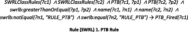
The explanation is the following (explanation about the comparison of names will be explained at the end of the section):
-
?c1 represents the company (X) and ?c2 represents the rest of the companies that are in the same sector of X.
-
?p1 represents the PTB of X and ?p2 the average PTB of the rest of the companies that are in the same sector of X.
The rule will be fired if ?p1 > = ?p2.
-


-
PER Premise/Rule:
The P/E ratio (price-to-earnings ratio) of a stock (also called its “P/E”, “PER”, “earnings multiple”, or simply “multiple”) is a measure of the price paid for a share relative to the annual net income or profit earned by the firm per share.
For this rule, it is necessary to calculate the average PER of all the companies that are in the same sector of “X” and the own PER value of “X”. Once we have both values, the rule will be fired if the PER of X is less or equal than the average of the sector.

The SWRL code of this rule is the following:

The explanation is the following (explanation about the comparison of names will be explained at the end of the section):
-
?c1 represents the company (X) and ?c2 represents the rest of the companies that are in the same sector of X.
-
?p1 represents the PER of X and ?p2 the average PER of the rest of the companies that are in the same sector of X.
The rule will be fired if ?p1 < = ?p2.
-


-
PER∩PTB Premise/Rule:
This rule will be fired if the two previous rules were fired.
The SWRL code of this rule is the following:

If both rules were fired (exists an instance in both classes), the PER intersection PTB rule is fired.

3.7.2 PCFR rule
The price/cash flow ratio (also called price-to-cash flow ratio or P/CF), is a ratio used to compare a company’s market value to its cash flow.
For this rule, it is necessary to calculate the average PCFR and PTB of all the companies that are in the same sector of “X” and the own PCFR and PTB value of “X”. Once we have both values, the rule will be fired if the PCFR of X is less or equal than the average of the sector and if the PTB of X is greater or equal than the average of the sector.

The SWRL code of this rule is the following:

The explanation is the following (explanation about the comparison of names will be explained at the end of the section):
-
?c1 represents the company (X) and ?c2 represents the rest of the companies that are in the same sector of X.
-
?p1 represents the PTB of X and ?p2 the average PTB of the rest of the companies that are in the same sector of X.
-
?pc1 represents the PCFR of X and ?pc3 the average PCFR of the rest of the companies that are in the same sector of X.
The rule will be fired if (?p1 > = ?p2) and (?pc1 < = ?pc3).
3.7.3 PTB ∩PCFR rule
This rule will be fired if the PCFR and PTB (PER∩PTB) rules were fired.
The SWRL code of this rule is the following:

If both rules were fired (exists an instance in both classes), the PTB intersection PCFR rule is fired.
If this rule is fired, that means that company X is a good company to invest in on a medium term place.
3.7.4 Long term prediction
The objective of this rule is comparing the calculated value called “Actual share calculated value” against the current value of the share of the company. Depending on the result of the comparison (one is greater than the other), one of the three investment options will be returned (sell, buy or maintain).
Before explaining in more detail the behavior of the rules, it is necessary to add some extra information about this rule. In this rule, we need to establish a margin value when we made comparisons with the Actual Share Calculated Value (ASCV). In this case, a margin value of 10% has been chosen. The margin will be of +10% in buy rule and −10% in sell rule. This means that the value of the ASCV that is stored in the ontology, in fact, is that value plus a 10% of itself. For example, if ASCV value is 19.450, the value that will be stored in the ontology when we fire the buy rule will be 21.395. In the sell rule, it will be 17.505.
This margin is used because fundamental analysis doesn’t try to calculate a concrete price to compare with the real price value. It tries to show a zone, a band of values in which the title price should move. For this reason, the system will use a margin of 10% over the calculated value.
-
Buy Rule:
This rule will be fired if the Actual Share Calculated Value (ASCV) is greater than the share value (SV) of the company.

The SWRL code of this rule is the following:

The explanation is the following (explanation about the comparison of names will be explained at the end of the section):
-
?c1 and ?c2 both represents the company (X), but, in this case, ?c1 instance will have stored the ASCV value and ?c2 the share value.
-
?vc1 represents the ASCV of X and ?pa1 the share value of X.
The rule will be fired if ?vc1 > ?pa1.
-


-
Sell Rule:
This rule will be fired if the Actual Share Calculated Value (ASCV) is less than the Share Value (SV) of the company.

The SWRL code of this rule is the following:

The explanation is the following:
-
?c1 and ?c2 both represents the company (X), but, in this case, ?c1 instance will have stored the ASCV value and ?c2 the share value.
-
?vc1 represents the ASCV of X and ?pa1 the share value of X.
The rule will be fired if ?vc1 < ?pa1.
-


-
Maintain Rule:
The maintain investment signal will be fired when Buy and Sell rule are fired at the same time. Thus, there is not a rule for Maintain.
-
Final explanation about string comparisons:
The comparisons between the names of the instances are made as a restriction. The objective of this comparisons is to check whether the variable ?n1, which contains the value of “name” property of the company instance (normally ?c1), doesn’t match with the string “RULE_X” where X is an identifier for the rule that the engine is processing. This string has been set at code level in order to identify the instance that stores the average value (or the actual share calculated value) of the different values. Thus, to have the rule completed to be fired, there is no need that the instance that identifies the company to invest contains the string of the rule. With that, inference problems are avoided.
4 Evaluation
The evaluation of the system needs to establish some previous considerations:
-
First of all, dividends will not be taken into account during the evaluation period in order to evaluate the goodness of the model. This is because the valuation method used to value the companies in the FAST system tries to establish an intrinsic value, that is, the value that in fact should have the share in function of its future capacity to generate rent. For that reason, the decision of the company regarding the distribution of the rent generated will not be taken into account.
-
In second place, FAST proposes a set of companies to perform an investment, keep the position or undo the investment in the short term. However, FAST does not suggest the weight that each investment should have. For that reason, FAST will assume that the investor will acquire a title of each share proposed. Thus, the comparison of the performance of these titles with the titles of an index will not take place, because in the titles of an index, the weight of each share is adjusted.
-
Performance restrictions have been identified in the literature as one of the main limitations of semantic technologies (e.g. [46–47]). Authors agree that, although this is a key aspect in the evolution of semantic technologies, the aims of the study presented in this paper do not include performance issues.
Once established the initial premises, FAST will be tested with real data based on the IBEX35 index (Spanish reference Index) (Fernandez and Yzaguirre 1995) to check the validity of its predictions.
4.1 Research design
Evaluation of the system will consist in the generation of two investment portfolios (IP). The reason for choosing this evaluation scheme is based on the recommendation of financial experts which considers that this type of evaluation is the best choice in this experimental setup. The First one (called IP A) will contain the recommendation that FAST provides us. This investment portfolio will be compared with the IP B. This portfolio will be obtained from IBEX35 index.
In order to choose a portfolio for the comparison, there are several options. The aim is to find a portfolio that could be chosen by a senior investor with the information that was available at that moment (this involves that the investor does not know which values are going to have the best performance at the end of the evaluation period).
Choosing a random portfolio does not make sense (this would not be a valid criterion for an investor) and comparing the FAST portfolio with a variable rent fund would not be commensurable, because these sorts of investments change their compositions almost every day and the weight of each value into the portfolio is adjusted.
Another option is to select an economic variable and choosing a percentage of the values that have the best data in relation with that variable. Nevertheless, this option involves several troubles. First of all, deciding what percentage of values should be selected would mean to add a subjective criterion.
On the other hand, even if it is possible to choose an objective percentage, it would necessary to decide which variable would be right. There are some considerations about this point. The first thing to keep in mind is that the evaluation period does not fit with the fiscal year (as it is explained below, on December of 2009 the composition of the index experienced a change).
All the economic variables included into the annual reports of the companies that compose the index are annual data and correspond to the fiscal year. But in order to publish this data, companies can wait until June. Thus, at the beginning of the evaluation period, the investor would not know this data. As an aggregate to this, basing a non-annual investment according only to a past annual variable does not seem to be the most rational criterion.
The composition of each portfolio is as follows:
-
Investment Portfolio A (IP A):
FAST will be fed with the necessary data to make predictions of all the companies that compose a concrete index (IBEX35) in a concrete day. FAST will return three types of recommendation: sell, maintain or buy. The IP A will be composed by a share of each company recommended by FAST.
-
Investment Portfolio B (IP B):
The IP B will be composed assuming that instead of following the recommendations made by FAST we will choose the option of invest directly in the index. This option avoids the problem of choosing subjective economic variables and percentages of values. It is just an objective, non random investment.
Nowadays is easy to find funds that invest only in variable rent. Some of them do it exclusively in all the values of the choose index. Not in vain, currently, there are more than one hundred funds that invest on Spanish variable rent. Many of them just replicate the index. For this reason, IP B is considered adequate for the FAST system. This option has been approved under the supervision of an expert on economics.
However, because of the reason exposed in the second premise, we will adopt a type of inversion where IP B will acquire a share of each of the titles that compose the index. Using this, the conditions of both portfolios will be equalized (they will not present weight). This will allow us to adjust both portfolios in order to equal their risks. As a consequence of this, there will be possible to perform egalitarian and objective comparisons among them.
Once created the two alternatives, three different tests will be made to compare and extract conclusions about which investment portfolio is better for an investor.
-
Test 1:
In this test a long term investment is faced. The investor is only interested in valuate the profitability in terms of the sell price given against the buy price. This kind of test is done to satisfy the needs of the sporadic investors. These investors are not intended to control the portfolio periodically; instead of this, they consider the investment in a long term approach.
The buy price of IP A is taken the same day of the recommendation (that is, the sum of the close prices of each of the titles). Also the price associated to the last day of the evaluation (that is, the sum of the close prices) will be obtained, allowing calculating the profitability. Finally, the buy price of IP B the recommendation day will be compared with the previously mentioned profitability. With this data we can extract the profitability of the portfolio.
-
Test 2:
In this test the daily profitability of the portfolio is controlled. This daily profitability should be given by the price of the shares that take part of the portfolio. The daily profitability of both portfolios (IP A and IP B) will be calculated as the average of the individual daily profitability’s of each one of the titles that are part of the portfolios. The operation will be repeated until the last day of validation period, where the average daily profitability will be obtained.
-
Test 3:
In this test, the concept of risk is introduced. In the previous test two different portfolios are confronted to judge those of them which can provide a higher profitability. In this case, risk is also taken into account. Each investment in a market assumes a risk. The general risk of the investment is called global risk and can be divided in two:
-
Systematic risk: It represents the part of the investment risk derived from the own dynamic of the market. This kind of risk is assumed by any title that quotes in any Stock Exchange and cannot be removed.
-
Specific risk: It represents the part of the risk that belongs to the title or titles and is independent of the market. It can be minimized with a correct diversification.
The IP B could be better diversified than IP A (unless FAST recommend us to invest in all the titles of the index, which will mean that both portfolios are identical), being necessary determinate the associated risk to both investments.
Once we determine the risk of each portfolio, the aim is to level both risks. Thus, an investor, at equal risk will prefer the portfolio that brings higher profitability.
Financial economy has provide us through the years some models that allows us to put two investments with a different risk level on a level to compare them directly. Given that M2 by Modigliani and Modigliani (1997) is one of the most popular models, this model will be adopted in Test 3.
-
4.2 Sample
Data was taken from IBEX35 stock market. The period used is the one that cover from the 9th of January 2009 to 1st of December 2009. At the beginning, it was considered to use a period equivalent to a natural year. However, in December 2009 some changes were introduced in IBEX35 stock market due to the fusion of the companies Ferrovial and Cintra and the entrance of the company Ebro Puleva in this stock market. To avoid consistency problems, it was decided to bring forward the test period.
Thus, the data set contains a total of 229 data (daily close prices) from each of the 35 entities that are part of the IBEX35 index, which means a total of 8,015 values. Apart from that, all the historic information that FAST can request to make their predictions were included in the system.
4.3 Results & discussion
The 35 companies that are part of the IBEX35 stock market are represented in Table 4:
In this scenario, the FAST system tends to recommend to invest in the following 8 companies represented in Table 5:
Portfolio IP A will be composed by a single share of each of these 8 companies. It will beat against portfolio IP B, composed by a single share of each of the 35 companies of the IBEX35.
-
Test 1:
This test will compare acquisition price and sell price. This requires calculating the buy prices of both portfolios to date 9th January of 2009 and the sell prices of the portfolios to 1st December of 2009. Results are showed in Table 6.
Table 6 Summarize of portfolios As we can see, FAST system would provide us a better investment alternative. Concretely, the IP A would allow us profitability 38.37% higher than IP B.
-
Test 2:
Table 7 shows the daily profitability’s the final profitability’s of the different portfolios at 1st December of 2009.
Table 7 Summarize of average daily profitability It is necessary to mention that the profitability’s of the table are daily means. Taking into account that we consider a long term investment, a difference in the daily profitability of 0.017% in the period, will equal to a differential of 3.89% in 229 days between IP A and IP B.
As can be appreciated, once more portfolio IP A beats portfolio IP B. In this case, the profitability would be a 28.81% higher. However, given that we can observe the daily behavior of both portfolios, it is possible to study the possible analogies between both alternatives. The comparison graph of both portfolios is showed in Fig. 4.
Fig. 4 
Comparison graph between portfolios according to their daily profitability
We proceed to the examination of the degree in which both portfolios are moving and oscillate in an analogous way through the calculus of the correlation coefficient. The result obtained is 0.091, which confirms that can be seen in the graphic: both portfolios have a high degree of lineal relation, moving in a very similar way.
Also, it has been studied through a t-Student if exists significance differences between the two variables. The result of the test (t(228) = 0.118, p > .05) indicates that doesn’t exist significance differences between both, which confirm the conclusions of the previous paragraph. However, it is important to note that, despite the similar tendencies, IP A yields better results in Test 2.

-
Test 3:
In Test 3 it is aimed to level risks between portfolios. In order to do so, Table 8 shows the standard deviation calculated over the daily profitability’s of both portfolios.
Table 8 Summarize of average daily profitability and standard deviation Results shows that IP A (less diversified), is more risky than IP B. Concretely, we assume a 3.82 more specific risk following FAST recommendations. We use the model M2 to adjust the profitability of portfolios and to be able to compare directly both portfolios as alternative investments fully comparables. Risk Adjusted Performance formula is as follows:
$$ {\text{M}}2\;{\text{or}}\;{\text{RAP}}\left( {{\text{Risk}}\;{\text{Adjusted}}\;{\text{Performance}}} \right) = \left( {{\sigma_{\text{M}}}/{\sigma_{\text{i}}}} \right)\left( {{{\text{r}}_{\text{i}}} - {{\text{r}}_{\text{f}}}} \right) + {{\text{r}}_{\text{f}}} $$Where
- σM :
-
is the standard deviation of the market return (of the benchmark) for the same period.
- σi :
-
is the standard deviation of the asset return
- ri :
-
is the asset return
- rf :
-
is the return of the free-risk asset (in this case, interest rate on 3 month Spanish government bond corrected to calculate their daily profitability. It has been selected the rate obtained after the auction of 17/12/2008 which is the current at the beginning of the evaluation period. Concretely the value was of 1.998% in 90 days, which is translated in a daily 0.02%).
After the application of the M2, the profitability of IP A has been reduced until a 0.074%. That means that now the portfolios A and B are exactly equals in risk and can be compared directly as analogous investments, being able to choose between them taking into account exclusively their profitability.
Under the previous conditions, IP A will be the preferred option of any investor which obey the criterions whose the economical theory define as rationality (that is, between two investments of same risk any rational individual would prefer always the one that gives a higher profitability). In this case, the profitability will be a 25.42% higher following the FAST recommendations.
Table 9 shows the results in the different Test sets.
Table 9 Differences between tests and portfolios The conclusion is that, under the initial premises, FAST will always offer a higher profitability to the alternative of making an investment in all the shares of the index. Profitability will be, in the worst case, a 25.42% higher and a 38.37% higher in the best scenario of the three studied. On the other hand, is striking the fact that, even being more risky to invest following FAST system (because it entails to assume a less diversification), comparing percentages, the difference is only a 3.82% and the coefficient of correlation rise to 0.91, being very next to the unit. Thus, FAST portfolio has resulted to be relatively diversified taking into account that is composed only of variable rent.
5 Conclusions and future work
The financial landscape has experienced a tremendous downturn in recent years. Economies going downhill and world-wide respected financial companies going bankrupt are just the tip of an iceberg of a global financial crisis that few were expecting some years ago. Given that situation, scientific methods for improving research in finance has recently gained momentum and promising new-cutting edge technologies such as traditional AI techniques applied to financial movements have leveraged the potential of upcoming finance-oriented Business Information Systems.
In this work, FAST, a promising approach for using semantics to harness trading recommendations through fundamental analysis is presented. Despite that this type of economic analysis being well-known for finance practitioners and researchers, in this paper, we summarized our work on how to bridge the gap between old-timer Fundamental Analysis based on ad-hoc studies on balances, assets and company ratios and current semantically-enriched descriptions of corporate parameters which could provide knowledge-based relationships and fine tuning for financial predictions.
The current work proposes three types of initiatives which should be explored in future research. In first place, the verification and validation of the FAST approach from an evaluation of financial prospective estimations standpoint. These works aim at implementing a wider range of functionalities which might range from including derivatives, swaps and a whole lattice of financial products to include more powerful algorithmic methods, which might be based on Support Vector Machines (SVMs) or a range of computational decidable formalisms that could improve the efficiency and accuracy of FAST. In second place, as stated before, semantic technologies are not the best technologies for the development of systems which needs a good temporal or spatial performance. However, future research will focus in the study of the performance of FAST compared with other similar but not semantic-enabled trading system. Finally, authors suggest extending the panoply of technologies adopted in FAST to include OWL 2 that, according to its specifications, could raise performance for semantic systems.
References
Abarbanell, J. S., & Bushee, B. J. (1997). Fundamental analysis, future earnings, and stock prices. Journal of Accounting Research, 35(1), 1–24.
Anastasakis, L., & Mort, N. (2009). Exchange rate forecasting using a combined parametric and nonparametric self-organising modelling approach. Expert Systems with Applications, 36(10), 12001–12011.
Broekstra, K., Kampman, A., Van Harmelen, F. (2002). Sesame: A generic architecture for storing and querying RDF and RDF schema. The Semantic Web—ISWC 2002. 2342, 54–68
Castells, P., Foncillas, B., Lara, R., Rico, M., & Alonso, J. L. (2004). Semantic web technologies for economic and financial information management. The Semantic Web: Research and Applications, 3053, 473–487.
Chavarnakul, T., & Enke, D. (2008). Intelligent technical analysis based equivolume charting for stock trading using neural networks. Expert Systems with Applications, 34(2), 1004–1017.
Chen, J. S., & Liao, B. P. (2007). Piecewise nonlinear goal-directed CPPI strategy. Expert Systems with Applications, 33(4), 857–869.
Chen, Y., Mabu, S., Shimada, S., & Hirasawa, K. (2009). A genetic network programming with learning approach for enhanced stock trading model. Expert Systems with Applications, 36(10), 12537–12546.
Fernandez Garcia, M. E., De la Cal Marin, E. A., & Quiroga Garcia, R. (2010). Improving return using risk-return adjustment and incremental training in technical trading rules with GAPs. Applied Intelligence, 33(2), 93–106.
Fernandez, P., & Yzaguirre, J. (1995). IBEX 35: Análisis e investigaciones. In: (Eds.), Barcelona: Ediciones Internacionales Universitarias
Fox, M. S., Barbuceanu, M., Gruninger, M., & Lin, J. (1998). An organizational ontology for enterprise modeling. Simulating organizations: Computational models of institutions and groups (pp. 131–152). Cambridge: MIT Press.
Gomez, J. M., García-Sanchez, F., Valencia-Garcia, R., Toma, I., Garcia-Moreno, C. (2009). SONAR: A semantically empowered financial search engine. International work-conference on the interplay between natural and artificial computation
Haarslev, V., & Möller, R. (2003). Racer: An OWL reasoning agent for the semantic web. Proceedings of the International Workshop on Applications, Products and Services of Web-based Support Systems
Horrocks, I., Patel-Schneider, P. F., Boley H., et al. (2004). SWRL: A semantic web rule language combining OWL and RuleML. W3C Member Submission
Jang, M., & Sohn, J. C. (2004). Bossam: An extended rule engine for OWL Inferencing. Rules and Rule Markup Languages for the Semantic Web, 3323, 128–138.
Kim, K. J. (2004). Toward global optimization of case-based reasoning systems for financial forecasting. Applied Intelligence, 21, 239–249.
Kovalerchuk, B., & Vityaev, E. (2000). Data mining in finance: Advances in relational and hybrid methods. Kluwer Academic
Lee, S. J., Ahn, J. J., Oh, K. J., & Kim, T. Y. (2010). Using rough set to support investment strategies of real-time trading in futures market. Applied Intelligence, 32(3), 364–377.
Lo, A., Mamaysky, H., & Wang, J. (2000). Foundations of technical analysis: Computational algorithm, statistical inference, and empirical implementation. Journal of Finance, 55(4), 1705–1765.
Losada, A. S., Bas, J. L., Bellido, S., Contreras, J., Benjamins, R., Gomez, J. M. (2005). Data, information and process integration with semantic web services
Majhi, R., Panda, G., Majhib, B., & Sahoo, G. (2009). Efficient prediction of stock market indices using adaptive bacterial foraging optimization (ABFO) and BFO based techniques. Expert Systems with Applications, 36(6), 10097–10104.
Majhi, R., Panda, G., & Sahoo, G. (2009). Development and performance evaluation of FLANN based model for forecasting of stock markets. Expert Systems with Applications, 36(3), 6800–6808.
Markowitz, H. (1952). Portfolio selection. Journal of Finance, 7, 77–91.
Markowitz, H. (1999). The early history of portfolio theory. Financial Analysts Journal, 55(4), 1600–1960.
McGuinness, D. L., & Harmelen, F. V. (2004). OWL web ontology language overview. W3C Recommendation
Mochón, A., Quintana, D., Sáez, Y., & Isasi, P. (2008). Soft computing techniques applied to finance. Applied Intelligence, 29(2), 111–115.
Modigliani, F., & Modigliani, L. (1997). Risk-adjusted performance. Journal of Portfolio Management, 23, 45–54.
Mossin, J. (1966). Equilibrium in a capital asset market. Econometrica, 34(4), 768–783.
Motik, B., & Studer, R. (2005). KAON2—a scalable reasoning tool for the semantic web. European Semantic Web Conference
Mullins, D. W. (1982). Does the capital asset pricing model work? Harvard Business Review, 105–113
Partridge, C., & Stefanova, M. (2001). A synthesis of state of the art enterprise ontologies. Lessons Learned. The BORO Program, LADSEB CNR
Qian, B., & Rasheed, K. (2006). Stock market prediction with multiple classifiers. Applied Intelligence, 26, 25–33.
Quah, T. S. (2009). DJIA stock selection assisted by neural network. Expert Systems with Applications, 35(1/2), 50–58.
Rodríguez-González, A., García-Crespo, Á., Colomo-Palacios, R., Guildrís-Iglesias, F., & Gómez-Berbís, J. M. (2011). CAST: Using neural networks to improve trading systems based on technical analysis by means of the RSI financial indicator. Expert Systems with Applications, 38(9), 11489–11500.
Roy, A. D. (1952). Safety first and the holding of assets. Econometrica, 20(3), 431–449.
Schumaker, R. P., & Chen, S. (2009). Textual analysis of stock market prediction using breaking financial news. ACM Transactions on Information Systems, 27(2)
Sharpe, W. F. (1966). Mutual fund performance. Journal of Business, 39(1), 119–138.
Shearer, R., Motik, B., Horrocks, I. (2008). HermiT: A highly-efficient OWL reasoner. In: A. Ruttenberg, U. Sattler, C. Dolbear (Ed.), Proc. of the 5th Int. Workshop on OWL: Experiences and Directions (OWLED 2008 EU)
Sirin, E., Parsia, B., Cuenca-Grau, B., Kalyanpur, A., & Katz, Y. (2007). Pellet: A practical OWL-DL reasoner. Web Semantics: Science, Services and Agents on the World Wide Web, 5(2), 51–53.
Sitte, R., & Sitte, J. (2002). Neural networks approach to the random walk dilemma of financial time series. Applied Intelligence, 16(3), 163–171.
Standfield, K. (2005). Intangible finance standards: Advances in fundamental analysis & technical analysis. Elsevier Academic Press
Vanstone, B., & Finnie, G. (2009). An empirical methodology for developing stockmarket trading systems using artificial neural networks. Expert Systems with Applications, 36(3), 6668–6680.
Vanstone, B., & Tan, C. N. W. (2005). Artificial neural networks in financial trading. In: M. Khosrow-Pour (Ed.), Encyclopedia of information science and technology. Idea Group
Wang, Y. F. (2003). Mining stock prices using fuzzy rough set system. Expert Systems with Applications, 24(1), 13–23.
Wen, Q., Yang, Z., Song, Y., & Jia, P. (2010). Automatic stock decision support system based on box theory and SVM algorithm. Expert Systems with Applications, 37(2), 1015–1022.
XBRL International. (2009). XBRL: eXtensible business reporting language. Retrieved June 19, 2009, from XBRL International Web site: http://www.xbrl.org
Yoda, M. (1994). Predicting the Tokyo stock market. In: G. J. Deboeck (Ed.), Trading on the edge (pp. 66–79). Wiley (1994)
Acknowledgements
This work is supported by the Spanish Ministry of Science and Innovation under the project TRAZAMED (IPT-090000-2010-007).
Author information
Authors and Affiliations
Corresponding author
Rights and permissions
About this article
Cite this article
Rodríguez-González, A., Colomo-Palacios, R., Guldris-Iglesias, F. et al. FAST: Fundamental Analysis Support for Financial Statements. Using semantics for trading recommendations. Inf Syst Front 14, 999–1017 (2012). https://doi.org/10.1007/s10796-011-9321-1
Published:
Issue Date:
DOI: https://doi.org/10.1007/s10796-011-9321-1