
Abstract
Relational learning algorithms mine complex databases for interesting patterns. Usually, the search space of patterns grows very quickly with the increase in data size, making it impractical to solve important problems. In this work we present the design of a relational learning system, that takes advantage of graphics processing units (GPUs) to perform the most time consuming function of the learner, rule coverage. To evaluate performance, we use four applications: a widely used relational learning benchmark for predicting carcinogenesis in rodents, an application in chemo-informatics, an application in opinion mining, and an application in mining health record data. We compare results using a single and multiple CPUs in a multicore host and using the GPU version. Results show that the GPU version of the learner is up to eight times faster than the best CPU version.
1 Introduction
Relational Learning is dedicated to model relationships among data items or attributes of databases. In contrast to standard learning, the relational learning process can find relations among attributes and/or among examples from multiple relational tables. Applications are very diverse, ranging from mining medical databases, to mining blogs, to chemo-informatics, to citation matching [25].
One very popular approach to relational learning is inductive logic programming (ILP) [12]. In this logic based framework, we are given a set of positive examples \(E^+\), a set of negative examples \(E^{-}\), a description of the examples in first order logic (background knowledge \(B\)), a language bias and a set of constraints. The goal is to find a first order logic hypothesis \(H\) that ideally covers (explains) all positive examples and none of the negative.
ILP has been quite successful in producing good classifiers as well as uncovering new knowledge from data. Most ILP systems operate by enumerating rules. In this case, the number of different rules, or the search space, can grow very quickly with the data size. Several techniques have been proposed to control the size of the search space and scale up ILP to larger data-sets [12]. One of them is to parallelize ILP. ILP parallelization can be done at several levels: nodes in the search space can be exploited in parallel [16, 31], the background knowledge can be partitioned and searched in parallel at the cost of incompleteness, or coverage of each new rule found can be performed in parallel [13]. In this work we concentrate on the paralelization of the coverage, which is one of the core steps in ILP. This step scores a new found rule by checking which examples are covered. It is well known that most of the computation time of an ILP system is spent on computing coverage [8].
We show that GPU processing has the capacity to expedite ILP execution by speeding-up coverage computation. Our approach interfaces Aleph [29], arguably the most popular ILP system, with our datalog engine for GPUs [22]. Because both Aleph and the datalog engine use a similar underlying logic representation, the interface is very tight. To run Aleph, we use the YAP prolog system [9]. At each Aleph coverage step, prolog compiles the rule found into a numerical representation that is passed to our GPU datalog engine. The resulting system maintains total compatibility with the original execution, and indeed could be easily adapted to most other ILP systems.
We tested our system with real-world ILP applications. Examples include two benchmarks from chemo-informatics, an application in opinion mining on a social network, and an application in mining health record data. We compare results using a single and multiple CPUs in the multicore host, and using a GPU. Overall, our GPU implementation often outperforms the highly optimized Aleph-YAP sequential implementation, and easily outperforms the multicore based implementation.
Section 2 presents background material to relational learning and the datalog language. Section 3 presents the design and implementation of our GPU-platform for relational learning applications, which consists of the Aleph ILP system, YAP prolog and our GPU-datalog engine. Section 4 presents an experimental evaluation of our platform. Section 5 presents related work and we conclude in Sect. 6.
2 Background
Relational Learning is the task of learning from databases. More precisely, we want to model relationships among data items from several tables (relations) in the database. Various forms of relational learning are discussed in the literature [12]. Inductive Logic Programming (ILP) is a very popular approach that employs a logic-based formalism, often based on subsets of first-order logic such as Horn clauses. Logic programs provide a highly flexible language. In contrast, domain-specific approaches, such as graph mining, obtain high performance by focusing on the more specific but very important task of searching for patterns in graphs [4]. Statistical Relational Learning [32] extends logic-based approaches by combining relational learning and probabilistic models.
Next we focus on ILP [12]. ILP depends on a logic-based data representation, that is often a datalog program.
2.1 Datalog
Datalog is a language based on first order logic that has been investigated as a data model for relational databases since the 80s [36, 37]. It has recently been used in new application domains including declarative networking, program analysis, distributed social networking, and security [21]. Interest in datalog has always stemmed from its ability to compute the transitive closure of relations through recursive queries which, in effect, turns relational databases into deductive databases, or knowledge bases. The renewed interest in datalog has in turn prompted new implementations of datalog targeting computing architectures such as GPUs [14, 20], field-programmable gate arrays (FPGAs) [21], and distributed computing based on Google’s MapReduce programming model [1].
A datalog program consists of a finite number of facts and rules. Facts and rules are specified using atomic formulas, which consist of predicate symbols with arguments [36].
As an example, we represent in datalog a subset of the organic molecule shown in Fig. 1. The molecule is represented as a set of atoms connected by bonds, also known as 2-D representation. Nodes represent atoms, and edges represent chemical bonds between atoms. The compound has three nitrogens, shown as N, and 11 carbon atoms, C, shown as unlabeled nodes.

2-D Representation of a small organic molecule
Using the datalog syntax we have the facts shown in Fig. 2. Each atom is identified by a two-attribute key consisting of a molecule identifier and an atom identifier. In the example, the atoms belonging to molecule d1 are identified as d1_1, d1_2 and d1_3. Each atom has its unique identifier, and its type, say c for carbon. Each relation in the database is called a predicate. In this case we have two relations atom/3 and bond/4, one describes the atoms in the molecule d1, and the other how d1’s atoms are bound together (a numerical representation). We use prolog notation, where names beginning with lower case letters refer to predicate names and constants, and names beginning with upper case letters are used for variables; numbers are considered constants. Each predicate is identified by its name and number of arguments (arity). Facts correspond to tuples. They consist of a single atomic formula (i.e., predicates with no connectives or subformulas and that do not depend on any other formula to be true), and their arguments are constants.

Extract of a prolog database representing the molecule in Fig. 1
The power of datalog resides in the ability to extend a database with Rules, that consist of two or more atomic formulas with the first one leftmost, called the rule’s head, separated from the other atomic formulas by the IF symbol :-. The other atomic formulas are subgoals separated by commas, which represent a logical AND. We will refer to all the subgoals of a rule as the body of the rule. Rules, in order to be general, are specified with variables as arguments, but can also have constants.
As a simple example, the next rule defines whether an atom \(A\) in molecule \(M\) has a neighboring nitrogen:

We use the bond relation to find the neighbor and atom to verify whether it is a nitrogen. Notice that, in this rule, we do not care about the type of a bond: this is represented by the _ symbol.
Rules can work together. In the next example, we use two rules to say that bonds are bidirectional:

Using this predicate we are guaranteed to work with an undirected graph, even if the data only includes one direction.
2.2 Inductive Logic Programming
The task of ILP is to learn new patterns that describe an unknown concept. Usually, the concepts will be learned by using examples: the set of positive examples, \(E^+\), that corresponds to valid instances, and the set of negative examples \(E^-\), that do not satisfy the concept. In the context of Fig. 1, the positive examples might be molecules (drugs) that cause cancer, and the negative examples are molecules that have no effect. In traditional learning, what we know about the example is in a single table. In ILP, we can use any fact or preexisting rule in the database. Moreover, we may set a number of constraints to the learning task, and we usually want to be able to shape the rules to learn.
More formally, ILP learns a theory \(H\) given a tuple \((E^+,E^-,B,L,C)\). The theory \(H\) we want to learn will usually be a set of rules \(\{R_1,\ldots ,R_n \}\). We want to cover or explain all positive examples in \(E^+\) and none of the negatives in \(E^-\). The background knowledge \(B\) is a program, a set of facts and rules that we believe to be true and relevant to the problem. The language bias, \(L\), defines the language of clauses that we can learn. Further reduction of the search space can be obtained by using the constraints \(C\).
2.3 ILP Search
In general, there is no constructive algorithm to obtain the best rules. Instead, ILP enumerates legal rules and selects the best one found. The most popular algorithm to learn a rule is shown in Algorithm 1. This algorithm is based on Progol’s [23]. Progol is one of the first ILP systems implemented. Aleph, the system used in this study, is based on Progol, and therefore, uses the same algorithm.

The process starts from an initial rule \(R_0\) and then keeps on searching until \(DoSearch()\) finds a high-quality clause. Three functions are critical to the algorithm. \(NextNode()\) (line 4) expands the current tree, often by expanding at the best node so-far. \(Better()\) (line 6) compares two sets of covered examples (counters are stored in variables \(P\), for the positive coverage, and \(N\), for the negative coverage, which ideally should be zero). Usually, this is done by simply computing a quality score, say, the difference between P and N (\(P-N\)). Last, \(Coverage\) (line 5) performs this task obtaining the set of examples that are explained by the rule (\(PCover\), \(NCover\)), and the counters, \(P\) and \(N\), for positive and negative examples, respectively.
Often we start with \(R_0\) as the rule that is always true. In the example domain, this corresponds to saying that all drugs cause cancer:

if we had 20 carcinogenic products (\(P=20\)) and 20 safe compounds (\(N=20\)), a possible initial score would be \(P-N=20-20=0\). To start searching, we include a body literal. Our language bias says that we need to use atoms first so we try

As we are looking at organic compounds, we still get \(P=20, N = 20\). We try nitrogen next:

and get \(P=18, N = 15\), a somewhat better result. Thus, \(NextNode()\) will start from the latter clause, say generating:

the process continues until we find a good clause, search the full space, or hit a stopping criteria.
Coverage computation (line 5 of Algorithm 1) is a key operation in this (and most) ILP algorithms, often dominating running time. Most often, it is implemented in prolog. Coverage is computed by matching an example against the head of the clause, and then proving each sub-goal in turn, left-to-right. Backtracking is needed if a non-leftmost subgoal fails: in this case we retry from the next solution of the sub-goal to left (or fail again). As soon as all sub-goals succeed, the example is covered and we stop. Prolog performance depends critically on indexing, and the YAP prolog system provides dynamic indexing that generates the best index for any type of call [7] in order to reduce coverage times.
Aleph implements a further optimization for coverage computation. The optimization is based on the observation that Horn clauses are monotonic. In other words, expanding a clause, that is, adding a literal may lead to less examples being covered, because the example may fail on the last goal, but if the example failed on the parent rule, it will fail on the expanded rule. Thus, Aleph maintains a coverage list for every node of the search space, and when expanding a node, it only checks the examples in this list. This is a classic time-space trade-off: it improves execution time by increasing memory usage.
The approach used by all ILP systems is top–down for the whole algorithm. In this setting, we execute the coverage step using a bottom–up approach in order to take advantage of data-parallelism that arises from a bottom–up computational model.
2.4 Evaluation of Datalog Programs
Datalog programs can be evaluated through a top–down approach or a bottom–up approach. The top–down approach (used by prolog) starts with the goal which is reduced to subgoals, or simpler problems, until a trivial problem is reached. It is tuple-oriented: each tuple is processed through the goal and subgoals using all relevant facts. Hence it is not easily adapted to GPU parallelism, because evaluating each goal can give rise to very different computations.
The bottom–up approach first applies the rules to the given facts, thereby deriving new facts, and repeating this process with the new facts until no more facts are derived. The query is considered only at the end, to select the facts matching the query. Based on relational operations (as described shortly), this approach is suitable for GPUs because such operations are set-oriented and relatively simple overall. Also, rules can be evaluated in any order. This approach can be improved using the magic sets transformation [2] or the subsumptive tabling transformation [33]. Basically, with these transformations the set of facts that can be inferred contains only facts that would be inferred during a top–down evaluation.
Bottom–up evaluation of datalog rules can be implemented using the relational algebra operators selection, join and projection, as outlined in Fig. 3. Selections are made when constants appear in the body of a rule. Next, a join is made between two or more subgoals in the body of a rule using the variables as reference. The result of a join can be seen as a temporary subgoal (or table) that has to be joined in turn to the rest of the subgoals in the body. Finally, a projection is made over the variables in the head of the rule.

Evaluation of a datalog rule based on relational algebra operations
For recursive rules, fixed-point evaluation is used. The basic idea is to iterate through the rules in order to derive new facts, and using these new facts to derive even more new facts until no new facts are derived [36].
2.5 GPU Architecture and Programming
GPUs are akin to Single-Instruction-Multiple-Data (SIMD) machines: they consist of many processing elements that run the same program but on distinct data items. This program, referred to as the kernel, can be quite complex including control statements such as if and while statements. However, a kernel is executed by groups of threads called warps [10]. These warps execute one common instruction at a time, so all threads of a warp must have the same execution path in order to obtain maximum efficiency. If some threads diverge, the warp serially executes each branch path, disabling threads not on that path, until all paths complete and the threads converge to the same execution path. Hence, if a kernel has to compare strings, processing elements that compare longer strings will take longer and other processing elements that compare shorter ones will have to wait.
GPU memory is organized hierarchically. Each (GPU) thread has its own per-thread local memory. Threads are grouped into blocks, each block having a memory shared by all threads in the block. Finally, thread blocks are grouped into a single grid to execute a kernel — different grids can be used to run different kernels. All grids share the global memory.
3 Our GPU-based Platform for Relational Learning
The main components of our platform are: the YAP prolog system [9], the Aleph ILP system [29], written in prolog, and a datalog engine for GPUs [22]. In contrast to our previous datalog engine design [22], in this design we can execute several queries at a time, and use various binary operators and prolog built-in predicates, such as the arithmetic built-ins necessary to process the relational learning applications using Aleph.
Aleph, YAP and the datalog engine interact as follows in running a relational learning application.
3.1 The Aleph Program and YAP Prolog
Figure 4 shows our GPU-based platform for relational learning from a high level perspective. The left block runs in a single host CPU core. First, the YAP prolog system reads/compiles the Aleph prolog program. Aleph has internal predicates that read from prolog datasets stored in disk. Besides, it implements predicates that perform the induce step that generates the rules. After induce is invoked, Algorithm 1 executes. For each rule found, YAP compiles the rule to the datalog engine representation and a sequence of kernels are used in the GPU side to compute the coverage of that rule.

GPU-based platform organization
When Aleph is initiated, YAP compiles all the facts of the dataset to the GPU representation. These facts, once sent to the GPU memory, tend to stay there until execution terminates. A memory management scheme swaps data between GPU memory and CPU memory, so that most recently used data remains in GPU memory. This tends to reduce the number of memory transfers (see Sect. 3.4 for more details).
Each unique string in a fact or rule is assigned a unique (integer) id; equal strings are assigned the same id. By using a numerical representation, our GPU kernels show relatively short and constant processing time because all tuples in a table, being managed as sets of integers, can be processed in the same amount of time. In contrast, if tuples were managed as strings, the processing of longer strings would take longer than shorter strings; thus slowing down our GPU kernel.
The datalog engine is developed in CUDA\(^{\textregistered }\).Footnote 1 The interface between YAP and CUDA includes three main functions: one to copy an extensional predicate from prolog to CUDA, one to install and uninstall a rule in CUDA, and one to invoke the CUDA datalog engine, returning a list with all solutions or a counter. In a normal datalog query, a dictionary is used at the very end, when the final results are to be displayed, to convert id’s to the corresponding strings that identify facts, rules and constants. In a normal Aleph execution, the results would be lists of positive and negative examples covered by the rule along with their counters, which would then be sent back to the host and converted to the corresponding strings using the dictionary. As mentioned in Sect. 2.3, these coverage lists are used by Aleph to avoid checking unnecessary examples when a new rule is generated. This reduces sequential execution time. In the context of this work, in order to take full advantage of the parallelization power offered by the GPUs, we do not use coverage lists. Instead, the datalog Engine always tests a rule against the whole set of examples, and only returns to the host the number of positive and negative examples covered by the rule. This eliminates the overhead of transferring coverage lists from the host to the GPU and vice-versa. Finally, there are predicates to initialise the datalog engine and to collect statistics. All these modifications are distributed with the YAP code and can be downloaded from http://www.dcc.fc.up.pt/~vsc/Yap/downloads.html.
We have also changed Aleph to compute coverage of a rule by calling the CUDA YAP interface.Footnote 2 In order to obtain coverage, we transform an Aleph generated rule such as:

into a coverage computing rule such as

where the table example is generated when loading the dataset and includes the primary key, the positive or negative polarity of the example, and the actual example. Evaluating the program materialises the covers table with the set of example identifiers and respective polarities, and we simply have to count to compute coverage.
3.2 The Host Thread of GPU-Datalog
The GPU-datalog engine consists of a single host thread and a number of GPU kernels. The host thread runs in the host platform (a multicore in our evaluation) and is responsible for various tasks, including the scheduling of the GPU kernels that implement the relational algebra operations selection, join and projection. We describe the GPU kernels in Sect. 3.5. The host thread is responsible for:
-
1.
Communicating with YAP both to receive the data to process (facts, rules, and queries in numerical format) and to send back results.
-
2.
Preprocessing the rules and facts (received from YAP) to send to the GPU, so that the GPU can process the data more efficiently. This preprocessing generates a numeric representation of the operations to be performed by the GPU kernels.
-
3.
Scheduling GPU work. This is supported by a memory management module described in Sect. 3.4.
3.3 Preprocessing
Datalog rules are evaluated by a sequence of GPU kernels that implement the relational algebra operations selection, join and projection. For the evaluation of each rule, the specification of what operations to perform, including constants, variables, facts and other rules involved, is carried out at the host (as opposed to be carried out in the GPU by each kernel thread), and sent to the GPU for all GPU threads to use. We next give a few examples of how the host specifies operations to the GPU.
Selection is specified by two values, column number to search and constant value to search; the two values are encoded as an array which can include more than one selection (more than one pair of values), as in the following example, where columns 0, 2, and 5 will be searched for the constants a, b and c, respectively:

Join is also specified by two values, column number in the first relation to join and column number in the second relation to join; the two values are sent as an array which can include more than one join, as in the following example, where the following columns are joined in pairs: column 1 in fact1 (variable X) with column 1 in fact2, column 2 in fact1 (variable Y) with column 4 in fact2, and column 3 in fact1 (Z) with column 0 in fact2.

Other operations are specified similarly with arrays of numbers. These arrays are stored in the GPU shared memory (as opposed to global memory) because they are small and the shared memory is faster.
3.4 Memory Management
A memory management module helps to identify the most recently used data within the GPU in order to maintain it in global memory and discard sections of data that are no longer necessary. Its purpose is to maintain facts and rule results in GPU memory for as long as possible so that, if they are used more than once, they may often be reused. To do so, we use an LRU algorithm in order to keep track of the GPU memory available, and maintain a list with information about each fact and rule result that is resident. When data (facts or intermediate tables) are requested to be loaded into GPU memory, they are first looked up in that list. If found, its entry in the list is moved to the beginning of the list; otherwise, memory is allocated for the data and a list entry is created at the beginning of the list. In either case, its address in memory is returned. If allocating memory for the data requires de-allocating other facts and rule results, those at the end of the list are de-allocated first until enough memory is obtained — rule results are written to CPU memory before de-allocating them. By so doing, most recently used fact and rule results are kept in GPU memory.
3.5 GPU Kernels of Relational Algebra Operators
Our GPU kernels include the relational algebra operators selection, join and projection to evaluate datalog programs and other supporting operators. All the data sent to the GPU is organized as arrays that are stored in global memory. The results of rule evaluations are also stored in global memory.
Rules are evaluated left to right. For each pair of subgoals \(G_l, G_k\) in a rule \(R\), we first apply selection (\(\sigma _{X_i=\mathtt c }(G_k)\)) and self-join (\(G_k \underset{X_i=X_j}{\bowtie } G_k\)) kernels to both subgoals in order to eliminate irrelevant tuples as soon as possible. They are followed by a join \(G_l \bowtie G_k\) kernel and then a projection kernel (\(\pi _{\setminus X_j}(G_{joinresult})\)) that eliminates unnecessary attributes. At the end of each rule evaluation, built-in predicates are performed followed by the duplicate elimination kernels.
A complete description of the algebra operators implementation design can be found in [22]. Next, we describe the implementation of additional operations, new to this datalog engine version.
3.6 Additional Operations
Many ILP programs require comparison predicates which were not part of our first, “Pure” datalog engine. Furthermore, the evaluation of the TPC-H queries (in Sect. 4.1) required the implementation of arithmetic predicates and aggregation. These new additions were implemented as follows:
-
Built-in comparison predicates (\(<,>,<>,=,>=,<=\)) Built-in comparison predicates are similar to the selection and self-join operations, i.e. they use a pipeline of three kernel executions. The first kernel marks all the rows that satisfy the comparison with one. The second kernel performs a prefix sum on these marks to determine the size of the result buffer and to use them as the indexes where each GPU thread must write its result. The third kernel writes the results. The difference is that comparison predicates use the given operator instead of always testing for equality. Also, they compare columns against a constant value (\(Y > 3\)) or against another column (\(Y > Z\)). The comparison predicates are performed at the end of each rule to ensure that their variables are assigned to a value. For example, consider the following rule:

the comparison \(Z > 3\) cannot be performed because we do not know the value of \(Z\) yet. Our engine, as part of the preprocessing step, rewrites the rule leaving that comparison at the end:

-
Arithmetic predicates (\(+, -, *, /\)) These predicates are performed after all joins and comparison predicates are completed (similar to the comparison predicates, they are moved to the end of the rule if necessary). Since the result size is always equal to the input size, they can be executed in a single kernel instead of the three kernels common in all other operations. Thanks to YAP’s “intelligent” analysis of rules, these predicates can be written in the usual infix notation and are automatically translated to postfix notation for easier evaluation. As an example on how to write arithmetic predicates, consider the rule:

Operations \(X + 3\) and \(Y / 5\) will be internally translated to \(X \, 3 \, +\) and \(Y \, 5 \, /\).
-
Aggregation (group by) and related operations (sum, avg, count) Aggregation is commonly used with other operations like summation, count, average, among others. It indicates a series of columns (variables in datalog) whose combined row values will determine the result of the related operations. They were implemented by adding a dummy predicate called aggregation that simply indicates the required variables. The related operations are represented by predicates with two values: the variable representing the input column and the one representing the output column. The related operations are performed by sorting the data according to the aggregation variables and then using Thrust’s reduce_by_key operation [34] with the sorted variables as keys. Note that reduce_by_key always performs a summation. However, count can be implemented by creating an additional column filled with 1’s and performing the summation on said column. The last operation, average, can be implemented by performing the summation on the required columns and then dividing the result by the result of the count. As an example, consider the rule:

with fact1 having the following values:
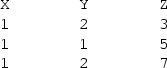
the result of the rule will be:


4 Experimental Evaluation
This section describes the platform, applications and experiments to evaluate the performance of our relational learning system that capitalises on GPUs.
4.1 Base Performance
In our previous work, we showed that our CUDA datalog implementation did very well at performing joins and transitive closures, easily outperforming other non-GPU based systems that use a top–down rule evaluation [22].
Similarly to our work, Diamos et al. [14, 15], Wu et al. [39, 41] and Young et al. [42] have also developed relational operators for GPUs, which are being integrated into the Red Fox [26] platform, an extended datalog developed by LogicBlox [18]. Their relational operators partition and process data in blocks using algorithmic skeletons. We compared our datalog GPU engine with the one used in the Red Fox platform. We used eight of the TPC-H [35] queries to evaluate the performance of our system: 1, 3, 4, 5, 10, 18, 19, 21, and manually translated them from SQL to datalog. Queries 2, 7, 9, 13, 14, 16, 20, 22 had sub-string operators (like, extract, substring). Since our system transforms whole strings into numbers, it was not possible for us to use these operators. Queries 6, 17 had floating-point constants and were not of interest to our work. Queries 8, 11, 12, 15 had operators that are hard to directly translate from SQL to datalog (case, having, views). The evaluation was performed in the same architecture described in [40], which includes a GeForce GTX TITAN, and used the same scale factor of 1 for TPC-H data which is roughly 1 GB. The tables were populated with random data using the TPC-H data generator, and that same scale factor.
Figure 5 shows the results of our system against the latest Red Fox results [26] with PCIe (GPU-bus) transfer time (i.e., time taken by memory transfers between the GPU and the host)—time spent on loading tables from disk to main memory is not included. Q1 shows roughly the same execution time for both Red Fox and our datalog engine. Our engine is faster for Q3 and Q19 and Red Fox is faster for the remaining five queries. Red Fox uses primitives of the ModernGPU library [28], which are well-tuned for coalesced memory accesses, while we use plain CUDA implementation. ModernGPU uses the Merge-Path framework [19, 24] to partition the data for Cooperative Thread Arrays (CTAs) and then threads so that the workload among the threads is balanced. Added to that, our system was optimised for logical queries, not SQL. Hence, query translation may also be sup-optimal.

Comparison between GPU-datalog and Red Fox
Regarding translation from SQL to logic queries, we believe that the main factor that affected the performance of our engine was query rewriting, particularly the use of auxiliary rules. For example, Q21 required two additional rules to represent two SQL exists operators. When these additional rules are evaluated, they create large intermediate tables which need to be joined to the main rule, increasing execution time. In contrast, three additional rules were created for Q19 to represent the or operator. These rules perform much better because their results are naturally fused together and are used into the main rule without the need to join.
In addition, the following factors contributed somewhat to the performance results of our system:
-
Comparison predicates These predicates are performed after all join operations are finished in order to ensure that their variables are assigned to a value. By correctly rearranging these predicates, their evaluation could be performed sooner, thus eliminating many unnecessary tuples earlier in the computation.
-
Join algorithm Red Fox has a slightly better join algorithm [14]. Therefore, since this algorithm computes the most time consuming operation, the benefits are significant.
4.2 Relational Learning: Materials and Methods
In this work we use the Aleph ILP system [29] to generate first order models for different domains. We performed experiments with three different versions of Aleph: (1) the original prolog code that runs relational learning applications in YAP, where coverage-lists are used to minimize the number of examples to be tested against a new rule (Aleph-cov), (2) a modified version of the original Aleph, where the whole set of examples is always passed to the coverage procedure (Aleph-all), and (3) a modified version of Aleph that calls the datalog engine to execute the coverage step, where the whole set of examples is used. For this version we use two different libraries: (3.1) that runs the coverage step on the GPU (Aleph-cuda) and (3.2) that runs the coverage step on the host multicore with several threads (Aleph-multi). The two first versions Aleph-cov and Aleph-all use a top–down approach to evaluate the queries. The other two, Aleph-cuda and Aleph-multi use a bottom-up approach using the datalog engine.
Aleph-multi is our multicore version of our datalog engine, which uses OpenMP. Its interface is similar to the Aleph-cuda interface. It uses the bottom–up approach and does not include any prolog optimizations like tabling or coverage lists. Like Aleph-cuda, it is based on the same relational algebra operations, with one major difference: instead of using three function calls (kernels) for selections and joins, we decided to capitalize on the CPU’s flexible memory scheme by using size-changing arrays. With these arrays, each thread can write a resulting tuple as soon as it is found, and the final result is given by joining all the arrays. This reduces the number of function calls to a single call, and therefore reduces processing time.
In discussing our experimental results below, Aleph-cov is used as a baseline comparison algorithm, because this is the sequential version that is normally used for relational learning tasks. We first compare the versions that run entirely on the host, Aleph-cov, Aleph-all (both top–down) and Aleph-multi (bottom–up), with one thread, to evaluate how the top–down and bottom–up evaluation behave on our relational learning applications. Next, we compare the results of our Aleph-cuda implementation with Aleph-cov, Aleph-all, and the best results obtained with Aleph-multi. We then evaluate the scalability of the Aleph-multi version with varying number of threads.
The first order models generated by all versions are the same as well as the counters of positive and negative examples. Each run was performed ten times. The reported execution times are averages of ten runs and are expressed in seconds. The standard deviation is low.
Next, we describe the relational learning applications we use in this work.
4.2.1 Applications
-
carcino: this is a well-known application that focuses on whether drugs may be carcinogenic in rodents. The ILP system has information on the drug’s 2-D structure (atoms and bonds) and on major chemical properties [30].
-
hiv: this dataset is based on the DTP AIDS anti-viral screen, that checks tens of thousands of compounds for evidence of anti-HIV activity. The ILP system has information on the drug compound’s 2-D structure [5, 38].
-
omop: this dataset consists of simulated medical records, namely diagnosis and prescription data. The task is to find drugs that can cause adverse side-effects, and it relies on temporal relationships between prescriptions and diagnosis [27].
-
blog: this is an application that contains collected blog postings about solar energy solutions taken from two Italian blog’s discussions/threads. Blogs are stored as a collection of Part-Of-Speech (POS) tokens. Further data on authorship, threading and title is also included in the analysis. The ILP task is to model blog’s author’s opinions [17].
These applications are characterized according to Table 1. Notice that the carcino is the smallest dataset. The other three applications have data bases with similar size, millions of tuples and tens of thousands of examples.
4.2.2 Hardware and Software
We used the following platform to run our experiments:
-
a host computer Core 2 Quad Processor Q9400 (4 cores in total) at 2.66 GHz, with:
-
4 \(\times \) 32 KB L1 instruction caches,
-
4 \(\times \) 32 KB L1 data caches,
-
2 \(\times \) 3 MB L2 caches (each cache shared between two cores),
-
6 GB DRAM,
-
a GeForce GTX 580, 1.54 GHz 512 CUDA Cores (16 Multiprocessors \(\times \) 32 CUDA Cores/MPK), 1535 MB GDDR5 memory, 768 KB L2 cache, CUDA Capability Major/Minor version number: 2.0. The software used was Ubuntu 12.04.1 LTS, gcc version 4.6.3, NVIDIA Corporation Cuda compilation tools, release 5.0, V0.2.1221, CUDA Driver Version/Runtime Version 5.0/5.0.
-
4.3 Relational Learning: Results
4.3.1 Aleph-cov, Aleph-all and Aleph-multi(1)
Table 2 shows the average execution times (in seconds) of all applications using three versions of Aleph (-cov, -all, -multi). As mentioned before, Aleph-cov is used as a reference since it is the system used for regular relational learning. We use Aleph-all to make a fair comparison with Aleph-cuda. Aleph-multi(1) is our multicore datalog engine using only one thread.
As expected, the execution times vary hugely from one application to another, since they present different characteristics (use of constants or built-in predicates, compound terms, etc.) and stress different parts of the YAP engine.
Since Aleph-cov does not use the whole set of examples to perform the coverage, its execution time is much lower than Aleph-all and Aleph-multi with one thread, but the difference in times vary according to the kind of application characteristic. For example, carcino, omop and blog benefit greatly from the coverage list optimization used by Aleph-cov.
4.3.2 Aleph-cuda, Aleph-all, Aleph-cov and Aleph-multi
Figure 6 shows the execution times of all applications using the four versions of Aleph, Aleph-cuda, Aleph-all, Aleph-cov and Aleph-multi. Results shown for Aleph-multi are the best for each application, being carcino’s best time obtained with one thread, hiv’s best time obtained with eight threads, and omop’s and blog’s best times obtained with four threads.

Applications total execution time for each Aleph version. Notice that the best times are obtained by the cuda engine in the three larger applications, even if bottom–up sequential execution is always slow
From the four applications, three of them greatly benefit from the CUDA implementation with speedups varying from 5 (blog) to 8.36 (omop), when comparing Aleph-cuda with the Aleph-cov version. The application carcino was the only one that did not benefit from the CUDA implementation. Its size caused the cost of memory transfers to dominate the total execution time.
One interesting observation is that Aleph-all, which somehow imitates the same coverage behaviour of Aleph-cuda, by not using the coverage-list, is still much slower than the CUDA and multicore versions. Note that the plots use logarithmic scale.
We instrumented our code to report the total amount of time spent in the GPU and in the different operations. Our results show that over 91 % of the running time is spent on the coverage step.
Figure 7 shows the time taken by the CUDA implementation in each datalog operation. There are six different steps. The first two perform all selections and self-joins required by the two sub-goals involved in each join. Next, an array is sorted to prepare for the join operation, then the join is performed. Finally, built-in predicates are evaluated (if any), followed by duplicate removal.

CUDA execution time breakdown
The applications have rather different characteristics. The carcino dataset, which did not benefit from the CUDA implementation spent most of its time in the join operation. In fact, join is one of the dominant operations for all applications together with selection. This is expected, since join is usually the most expensive operation in database processing. The hiv application is from a similar domain, chemo-informatics, but it is much less about joins: in fact the main operation is duplicate removal. A detailed analysis shows that the two applications use different representations for a molecule: hiv fuses bonds and atoms into a single table. This was developed to simplify prolog indexing, but seems to also result in smaller intermediate tables.
The blog and omop applications have the most well-balanced execution. Both datasets use many constants in the rules, and include self-joins, so the major component is indeed preparing each sub-goal join. The joins themselves are noticeably fast, as they do not take much more time than sorting or duplicate removal. This is probably because the main tables have strong functional dependencies in both cases. Notice that omop has a similar profile to blog, even if speed-ups are much worse. Last, omop uses comparisons to establish temporal precedence and is thus the only dataset where built-ins play a significant role.
4.3.3 Aleph-multi
In this section we compare our datalog engine implemented in a multicore machine with our sequential versions and our Aleph-cuda version.
Table 3 shows the average execution times of Aleph-multi for a varying number of threads for the four applications. Speedups (slowdowns) related to the Aleph-all and Aleph-cov versions, respectively, are between parentheses.
Comparing the results of Table 3 with the results shown in Table 2, we can observe that the prolog top–down execution with coverage lists (Aleph-cov) is the best for all applications. Bottom–up multicore datalog (Aleph-multi) outperforms normal prolog (Aleph-all) in all applications except carcino, where it also suffers from carcino’s small size. These results show that coverage lists are more important than the language (datalog vs. prolog) or the evaluation method (top–down vs. bottom–up).
However, our most important conclusion is that our Aleph-cuda implementation performs much better on these applications exploiting more efficiently the GPU resources than our multicore implementation, Aleph-multi, exploiting the multicore resources. Because the coverage step presents a tendency to produce finer-grained tasks, the results are somewhat better on the GPU, with maximum speedup of 8, while our multicore implementation has a maximum speedup of 4.
5 Related Work
He et al. [20] have designed, implemented and evaluated GDB, an in-memory relational query co-processing system for execution on both CPUs and GPUs. GDB consists of various primitive operations (scan, sort, prefix sum, etc.) and relational algebra operators built upon those primitives.
We modified the Indexed Nested Loop Join (INLJ) of GDB for our single join and multi-join, so that more than two columns can be joined, and a projection performed, at the same time. Their selection operation and ours are similar too; ours takes advantage of GPU shared memory and uses the Prefix Sum of the Thrust Library. Our projection is fused into the join and does not perform duplicate elimination, while they do not use fusion at all.
As mentioned in Sect. 4.1, Diamos et al. [14, 15], Wu et al. [39, 41] and Young et al. [42] have developed relational operators for GPUs. Their join algorithm, compared to that of GDB, shows 1.69 performance improvement [14]. Their selection performs two prefix sums and the result is written and then moved to eliminate gaps; our selection performs only one prefix sum and writes the result once. They discuss kernel fusion and fission in [41]. We applied fusion (e.g., simultaneous selections, selection then join, etc.) at source code, while they implement it automatically through the compiler. Kernel fission, the parallel execution of kernels and memory transfers, is not yet adopted in our work.
With respect to running relational learning algorithms in GPUs, to the best of our knowledge, this is the first attempt. Regarding parallelization of the coverage algorithm using a multicore implementation and top–down evaluation, Côrte-Real et al. [6] managed to achieve linear speedups using a multi-threaded implementation. However, the execution times reported are only on the coverage step and ignore all other Aleph operations. Other attempts were done on distributed environments with modest speedups [16, 31].
6 Conclusions
To the best of our knowledge, we presented the first attempt to run relational learning algorithms, based on ILP, on GPU platforms. Our relational learning setting for GPUs takes advantage of already available systems: the YAP prolog system, the Aleph ILP system and a datalog engine for GPUs, in order to speed-up the execution of the main core of an ILP algorithm, the coverage step. Using the GPU required minimal changes to the relational learning system while preserving the original search-space. Our results show a performance improvement for three of the four relational learning applications, varying between 5 and almost 8.5. These results were compared to the results obtained with a version of the relational learning coverage step implemented for multicores, and the GPU version achieved better maximum speedups. We believe that these results can be further improved, and we have been working on the following extensions to our datalog GPU engine.
-
Managing tables larger than the total amount of GPU memory.
-
Mixed processing of rules both on the GPU and on the host multicore.
-
Improved join operations to eliminate duplicates earlier in the computation.
-
Improved GPU memory management according to recent progress in this area [11].
GPUs are nowadays widely used for traditional machine learning algorithms [3]. Our results show that GPUs are also a natural fit to multi-relational learning tasks, and should be considered for other multi-relational computationally intensive tasks. The same framework used here can be reused for other logic-based relational learners.
Notes
CUDA is NVIDIA’s General-Purpose Parallel Computing Platform and Programming Model [10].
The Aleph modified version is available upon request to the authors.
References
Afrati, F.N., Borkar, V., Carey, M., Polyzotis, N., Ullman, J.D.: Cluster computing, recursion and datalog. In: Proceedings of the First International Conference on Datalog Reloaded, Datalog’10, pp. 120–144. Springer, Berlin (2011)
Beeri, C., Ramakrishnan, R.: On the power of magic. J. Log. Program. 10(3&4), 255–299 (1991)
Bekkerman, R., Bilenko, M., Langford, J. (eds.): Scaling up Machine Learning: Parallel and Distributed Approaches. Cambridge University Press, Cambridge (2011)
Chakrabarti, D., Faloutsos, C.: Graph mining: laws, generators, and algorithms. ACM Comput. Surv. 38(1) (2006). doi:10.1145/1132952.1132954
Collins, J.M.: The DTP AIDS antiviral screen program (1999). http://dtp.nci.nih.gov/docs/aids/aidsdata.html
Côrte-Real, J., Dutra, I., Rocha, R.: A map-reduce constructor for prolog. In: Proceedings of the International Conference on Principles and Practice of Declarative Programming (PPDP) (2013)
Costa, V.S., Sagonas, K., Lopes, R.: Demand-driven indexing of prolog clauses. In: Veronica D., Ilkka N. (eds.) Proceedings of the 23rd International Conference on Logic Programming, volume 4670 of Lecture Notes in Computer Science, pp. 305–409. Springer (2007)
Costa, V.S., Srinivasan, A., Camacho, R., Blockeel, H., Demoen, B., Janssens, G., Struyf, J., Vandecasteele, H., Van Laer, W.: Query transformations for improving the efficiency of ilp systems. J. Mach. Learn. Res. 4, 465–491 (2003)
Costa, V.S., Rocha, R., Damas, L.: The yap prolog system. Theory Pract. Log. Program. 12(1–2), 5–34 (2012)
CUDA C programming guide. http://docs.nvidia.com/cuda/cuda-c-programming-guide/index.html
Dastgeer, U., Li, L., Kessler, C.: Smart containers and skeleton programming for GPU-based systems. In: Proceedings 7th International Symposium on High-Level Parallel Programming and Applications (HLPP’14), Amsterdam (2014)
De Raedt, L.: Logical and Relational Learning. Springer, Berlin (2008)
Dehaspe, L., De Raedt, L.: Parallel inductive logic programming. In: In Proceedings of the MLnet Familiarization Workshop on Statistics, Machine Learning and Knowledge Discovery in Databases, pp. 112–117 (1995)
Diamos, G., Wu, H., Lele, A., Wang, J., Yalamanchili, S.: Efficient relational algebra algorithms and data structures for GPU. Technical report, Georgia Institute of Technology (2012)
Diamos, G., Wu, H., Wang, J., Lele, A., Yalamanchili, S.: Relational algorithms for multi-bulk-synchronous processors. In: Proceedings of the 18th ACM SIGPLAN Symposium on Principles and Practice of Parallel Programming, PPoPP ’13, New York, NY, USA, pp. 301–302. ACM (2013)
Fonseca, N.A., Srinivasan, A., Silva, F.M.A., Camacho, R.: Parallel ILP for distributed-memory architectures. Mach. Learn. 74(3), 257–279 (2009)
Gavanelli, M., Riguzzi, F., Milano, M., Cagnoli, P.: Constraint and optimization techniques for supporting policy making. In: Yu, T., Chawla, N., Simoff, S. (eds) Computational Intelligent Data Analysis for Sustainable Development, Data Mining and Knowledge Discovery Series, chap. 12, pp. 361–382. Chapman & Hall/CRC, Abingdon (2013)
Green, T.J., Aref, M., Karvounarakis, G.: Logicblox, platform and language: a tutorial. In: Proceedings of the Second International Conference on Datalog in Academia and Industry, Datalog 2.0’12, pp. 1–8. Springer, Berlin (2012)
Green, O., McColl, R., Bader, D.A.: GPU merge path: a GPU merging algorithm. In: Proceedings of the 26th ACM International Conference on Supercomputing, ICS ’12, New York, NY, USA, pp. 331–340. ACM (2012)
He, B., Mian, L., Yang, K., Fang, R., Govindaraju, N.K., Luo, Q., Sander, P.V.: Relational query coprocessing on graphics processors. ACM Trans. Database Syst. 34(4), 21:1–21:39 (2009)
Huang, S.S., Green, T.J., Loo, B.T.: Datalog and emerging applications: an interactive tutorial. In: Proceedings of the 2011 ACM SIGMOD International Conference on Management of Data, SIGMOD ’11, New York, NY, USA, pp. 1213–1216. ACM (2011)
Martínez-Angeles, C.A., Dutra, I., Costa, V.S., Buenabad-Chávez, J.: A datalog engine for GPUs. In: WFLP-2013: 22nd International Workshop on Functional and (Constraint) Logic Programming, Kiel, Germany, 11–13 Sept, pp. 239–253 (2013)
Muggleton, S.: Inverse entailment and progol. New Gener. Comput. 13, 245–286 (1995)
Odeh, S., Green, O., Mwassi, Z., Shmueli, O., Birk, Y.: Merge path—parallel merging made simple. In: Proceedings of the 2012 IEEE 26th International Parallel and Distributed Processing Symposium Workshops & PhD Forum, IPDPSW ’12, Washington, DC, USA, IEEE Computer Society, pp. 1611–1618 (2012)
Rajaraman, A., Ullman, J.D.: Mining of Massive Datasets. Cambridge University Press, Cambridge (2012)
Red fox: a compilation environment for data warehousing. http://gpuocelot.gatech.edu/projects/red-fox-a-compilation-environment-for-data-warehousing/
Ryan, P.B., Schuemie, M.J.: Evaluating performance of risk identification methods through a large-scale simulation of observational data. Drug Saf. 36(1), 171–180 (2013)
Sean Baxter: modern GPU library—tutorial. http://nvlabs.github.io/moderngpu/index.html (visited in Jan 2015) (2013)
Srinivasan, A.: The Aleph manual. University of Oxford, England (2001). http://www.cs.ox.ac.uk/activities/machlearn/Aleph/aleph.html
Srinivasan, A., King, R.D., Muggleton, S.H., Sternberg, M.J.E.: Carcinogenesis predictions using ILP. In: Lavrac, N., Dszeroski, S. (eds.) Inductive Logic Programming, volume 1297 of Lecture Notes in Computer Science, pp. 273–287. Springer, Berlin (1997)
Srinivasan, A., Faruquie, T.A., Joshi, S.: Data and task parallelism in ILP using MapReduce. Mach. Learn. 86(1), 141–168 (2012)
Taskar, B., Getoor, L.: Introduction to Statistical Relational Learning. MIT Press, Cambridge (2007)
Tekle, K.T., Liu, Y.A.: More efficient datalog queries: subsumptive tabling beats magic sets. In: SIGMOD Conference, pp. 661–672 (2011)
Thrust: a parallel template library. http://thrust.github.io/
TPC-H transaction processing performance council benchmark H. http://www.tpc.org/tpch/
Ullman, J.D.: Principles of Database and Knowledge-Base Systems, vol. I. Computer Science Press, Rockville (1988)
Ullman, J.D.: Principles of Database and Knowledge-Base Systems, vol. II. Computer Science Press, Rockville (1989)
Weislow, O.S., Kiser, R., Fine, D.L., Bader, J., Shoemaker, R.H., Boyd, M.R.: New soluble-formazan assay for hiv-1 cytopathic effects: application to high-flux screening of synthetic and natural products for aids-antiviral activity. J. Natl. Cancer Inst. 81(8), 577–586 (1989)
Wu, H., Diamos, G., Cadambi, S., Yalamanchili, S.: Kernel weaver: automatically fusing database primitives for efficient GPU computation. In: Proceedings of the 2012 45th Annual IEEE/ACM International Symposium on Microarchitecture, MICRO-45, Washington, DC, USA, IEEE Computer Society, pp. 107–118 (2012)
Wu, H., Diamos, G., Sheard, T., Aref, M., Baxter, S., Garland, M., Yalamanchili, S.: Red fox: an execution environment for relational query processing on gpus. In: International Symposium on Code Generation and Optimization (CGO) (2014)
Wu, H., Diamos, G., Wang, J., Cadambi, S., Yalamanchili, S., Chakradhar, S.: Optimizing data warehousing applications for gpus using kernel fusion/fission. In: Proceedings of the 2012 IEEE 26th International Parallel and Distributed Processing Symposium Workshops & PhD Forum, IPDPSW ’12, Washington, DC, USA, IEEE Computer Society, pp. 2433–2442 (2012)
Young, J., Wu, H., Yalamanchili, S.: Satisfying data-intensive queries using GPU clusters. In: 2012 SC Companion High Performance Computing, Networking, Storage and Analysis (SCC), pp. 1314–1314 (2012)
Acknowledgments
The authors gratefully acknowledge the comments from all reviewers, which highly improved the quality of this paper. We would also like to thank Martínez-Angeles’ M.Sc. and qualification committee members for their helpful comments.
Author information
Authors and Affiliations
Corresponding author
Additional information
CMA was supported by the University of Porto, the Centre for Research and Postgraduate Studies of the National Polytechnic Institute (CINVESTAV-IPN) of Mexico, and the Council of Science and Technology (CONACyT) of Mexico. ICD and VSC were partially supported by: the European Regional Development Fund (ERDF), COMPETE Programme; the Portuguese Foundation for Science and Technology (FCT), projects ADE (PTDC/EIA-EIA/121686/2010 (FCOMP-01-0124-FEDER-020575)), and ABLe PTDC/EEI-SII/2094/2012.
Rights and permissions
About this article

Cite this article
Martínez-Angeles, C.A., Wu, H., Dutra, I. et al. Relational Learning with GPUs: Accelerating Rule Coverage. Int J Parallel Prog 44, 663–685 (2016). https://doi.org/10.1007/s10766-015-0364-7
Received:
Accepted:
Published:
Issue Date:
DOI: https://doi.org/10.1007/s10766-015-0364-7