
Abstract
The water inrush of roof induced by mining was related to the height of water flowing fractured zone under large-scale water bodies. Based on the drilling revealed stratum, the thickness of different overlying layers was obtained within the scope of Santaizi reservoir. The height of water flowing fractured zone of different workface on the outside of reservoir under the condition of fully mechanized level mining area was the prediction sample, the generalized analysis of sensitive factors that affected the development of water flowing fractured zone was carried on. The mining depth, dip angle of coal seam, mudstone ratio, compressive strength, mining thickness and the inclined length of the goaf were selected as the influence factors to predict the height of water flowing fractured zone. The height of water flowing fractured zone of unmined working face within the scope of Santaizi reservoir was obtained by objective entropy method. The index weight value of each influence factor was determined. The thickness of the different overlying rock layers above water flowing fractured zone was obtained. And the safety evaluation of water-inrush of unmined working face within the scope of Santaizi reservoir was studied. The important parameter and technical support were provided for the rational design and mining of the working faces under the reservoir.
1 Introduction
The mining under water body can lead to the growth of water flowing fracture zones, when the water flowing fracture zones connected the upper water, the groundwater would inrush into the working face and brought serious safety hazards to the production of the mine with the improve of mechanization degree of coal mining (Wang 2006; Li and Li 2012). Therefore, it was very important to study the development law of water flowing fracture zones under the influence of multiple factors. The height and shape of water flowing fractured zone was the key to ensure safety mining under water bodies. Currently the prediction methods of the height of water flowing fractured zone were divided into similar simulation experiment (Lin et al. 2010; Zhao et al. 2011; Gao and Wu 2011), theoretical analysis (Xu and Sun 2011; Shi et al. 2012), field testing (Luan et al. 2010; Kang et al. 2009). But these methods were obvious limitations. The empirical formula based on large number of data was not sufficient to adapt to complex mining conditions (Wang 2006). To make up the shortcoming of the above methods, Chen et al. (2005) used nonlinear artificial neural network to objectively describe the relationship between the height of water flowing fractured zone and the mechanical properties of the roof. Ding et al. (2005) established a subtraction clustering model to predict the height of the water flowing fractured zone based on the adaptive neural fuzzy system. Cheng et al. (2011) established the stability evaluation model of goaf and predicted the height of the water flowing fractured zone based on the correlation degree of each factor by grey correlation method. Ma et al. (2013) and Pan (2009) analyzed the development rule of the water flowing fractured zone by the curve estimation and orthogonal test on the basis of the discrete element simulation. Hu et al. (2012) got a nonlinear statistical relation between the height of the water flowing fractured zone and multiple factors by multiple regression analysis. These improved the reliability of the prediction of the height of the water flowing fractured zone. The simplicity of the model varied from person to person owing to the difference of the fault, mining method, the mechanics properties of rock mass, the hydrological conditions et al. The determination of the weight of all indexes in the evaluation system relied on the expert’s subjective opinions. This affected the accuracy of the evaluation and lead to the deviation of the results. Therefore, the objective method was urgently needed for the quantitative study of the height of the water flowing fractured zone.
The authors introduced the objective entropy theory (Liang et al. 2010; Wang et al. 2012). The height of water flowing fractured zone of different workface on the outside of reservoir under the condition of fully mechanized level mining area was the prediction sample, the generalized analysis of sensitive factors that affected the development of water flowing fractured zone was carried on. The mining depth, dip angle of coal seam, mudstone ratio, compressive strength, mining thickness and the inclined long of the goaf were selected as the influence factors to predict the height of water flowing fractured zone. The height of water flowing fractured zone of unmined working face within the scope of Santaizi reservoir was obtained by objective entropy method. The index weight value of each influence factor was determined. The thickness of the different overlying rock layers above water flowing fractured zone was obtained. This study enriched the method of preventing water damage of the roof and had practical guiding significance for the safety production of deep mining under the water body.
2 Analysis of Hydrogeological Conditions in Daping Coal Mine
There are two minable coal seam of Nos. 1 and 2 coal seam in Daping mine field. The thickness of minable coal was about 0.80–12.0 m. The 3D geological model map of the strata in the Daping coal field was shown in Fig. 1. It can be seen that the main structural form was the Santaizi syncline. The geotectonic position of the basin was located in the composite location of the subsidence belt and the structural belt. The bottom of Santaizi reservoir generally was saturated loose silty sand with the thickness of 0.2 m. The permeability coefficient was about 0.04–1.01 m/d. The layers in the deep of 0.2–2.66 m were made up of subclay and clay which were impervious and aquifer. The permeability coefficient was about 0.002–0.34 m/d. The direct water filled aquifers in the coal field were mainly composed of cretaceous coarse sandstone and weak fractured pore bearing aquifers in sand conglomerate. The fault zone leaded to very weak water, and had no hydraulic connection with the surface water and the aquifers. The overlying rock was damaged owing to the mining of the working face. It was possible to increase the water permeability of the working face, and there was a serious hidden danger of water permeability.

The 3D geological model map of the strata in the Daping coal field
The thickness contour of overburden and the layout of working face in Daping coal field were shown in Fig. 2. It can be seen that The Santaizi reservoir was located in the middle of Daping coal field. The area of Santaizi reservoir was 1/3 of the area of Daping coal field. The industrial reserves within the scope of Santaizi reservoir accounted for nearly 1/2 of whole well reserves.

The thickness contour of overburden and the layout of working face in Daping coal field (unit: m)
The statistics of drilling revealed stratum within the scope of reservoir in Daping coal field was shown in Table 1. The thickness contour of water blocking layers and permeable layers within the scope of Santaizi reservoir was shown in Figs. 3 and 4. It could be seen that the thickness of overburden near the working face of N1S3, N1S4, S1S5 and S1S4 was relatively thin. The thinnest thickness of overburden was about 250 m near the No. 440 borehole. The thickness of water blocking layers (mudstone and fine siltstone) was about 180 m. The thickness of permeable coarse sandstone layers was about 80 m. The total thickness of the fine sandstone and mudstone near the No. 438 borehole was about 140 m. The thickness of fine sandstone and mudstone in the four working faces was about 160–200 m.

The thickness contour of permeable layers within the scope of reservoir

The thickness contour of water blocking layers within the scope of reservoir
3 The Prediction of the Height of Water Flowing Fractured Zone by Entropy Weight Evaluation Method
The acquisition of the height of water flowing fractured zone of the working face was very difficult by using ground water injection method under the Santaizi reservoir. The authors introduced the measured data of the height of water flowing fractured zone of working faces outside reservoir. The height of water flowing fractured zone of unmined working faces within the scope of the reservoir was obtained by entropy weight evaluation method Based on the relevance of the height of water flowing fractured zone with geological conditions, coal seam and roof mechanical condition and mining activities.
3.1 The Selection of Prediction Index of the Height of Water Flowing Fractured Zone
According to the practice experience in the production of coal mining, the main influence factors of the height of water flowing fractured zone were
-
1.
The environment of coal strata.
It concluded the thickness, angle and depth of coal seam.
-
2.
The mechanical characteristics of coal strata.
It concluded the crushing degree of roof, the hardness of roof, the compressive strength of overburden and the structure of overburden. the thickness, angle and depth of coal seam.
-
3.
Mining activities.
It concluded the mining thickness, the number of stratification, the size of working face and the management of roof.
The management of roof in Daping coal mine was all caving method. Due to the data similarity of adjacent working face, the mining depth, dip angle of coal seam, mudstone ratio, compressive strength, mining thickness and the inclined length of the goaf were selected as the influence factors to predict the height of water flowing fractured zone. The height of water flowing fractured zone was calculated by Matlab program. The predicted samples for the height of the water flowing fractured zone in adjacent working faces were shown in Table 2.
3.2 The Evaluation Model of Index System Based on Entropy Weight Method
Entropy was a function of describing the state of material system and the determination of the entropy weight coefficient was objectively dependent on the intrinsic information of the material. For a certain index, the greater the difference between the indicators was, the smaller the entropy was. The greater the weight of the index in the evaluation system was. If the difference of all indicators was zero, the function of the index in the evaluation system was 0. The calculation method was as follows:
There were n evaluation indexes and m was evaluated object. The original data of the corresponding indexes of the evaluated object were expressed in the form of the following matrix.
Firstly, the raw data was dimensionless processing.
The optimal value for each column in R was
Note: the benefit index was the better when the index value was the greater, the cost index was the better when the index value was the smaller.
When the original data was dimensionless, it was recorded as a matrix \(S = \left( {s_{ij} } \right)_{m * n}\).
Then, normalization of S
\(S_{ij}^{'} \in \left[ {0,1} \right]\) was obtained and did not destroy the proportion of data.
The entropy of the evaluation index of j was defined as
where \(t_{ij} = \frac{{S_{ij}^{\prime}}}{{\sum\nolimits_{i = 1}^{m} {S_{ij}^{\prime}}}}\) (j = 1,2,…, n), \(k = \frac{1}{\ln m}\) (this selection of K made \(0 \le H_{j} \le 1\)).
The difference coefficient of evaluation index j was defined as
The entropy weight of the evaluation index of j was
The defined entropy weight in the way had the following properties:
-
1.
When the value of each evaluated object on index J was the same, the entropy value reached the maximum value 1 and the entropy weight is zero, which means that the index did not provide any useful information to decision-makers, which could be considered to be canceled.
-
2.
When the value of each evaluated object on the index J was the larger difference, the entropy value was smaller and the entropy weight was larger. This means that the index provided useful information to decision-makers, and in this problem, there was obvious difference between each object on this index, so we should focus on it.
-
3.
The greater the entropy of the index was, the smaller the entropy weight was, the less important the index was. The entropy defined by the formula (7) satisfied the following conditions.
$$0 \le \omega_{j} \le 1,\,{\text{and}}\,\sum\limits_{j = 1}^{n} {\omega_{j} = 1} .$$
Entropy weight method calculated the weight of index based on the local differences, which reflected its importance by the degree of difference between the observed values of the same index.
The evaluation value of each object was calculated the following formula.
According to the size of \(x_{i}\), each evaluation object was evaluated. The bigger \(x_{i}\) was, the better the i object was.
The extreme value method was used to deal with the original data without dimensionalization.
The normalization matrix of S was calculated and recorded as S’
The entropy H of each index was calculated
The difference coefficient α of each index was calculated
The entropy weight W of each index was calculated
Through the calculation, it can be seen that
-
1.
The inclined length of the working face had the greatest influence on the height of water flowing fractured zone. When the overlying rock was not fully mined, the size of the goaf played a major role. And the weight of the index was 0.236. The size of goaf did not play a role in the non full extraction conditions. The height of water flowing fractured zone was lower in the full extraction conditions than that in the non full extraction conditions. There was non sufficient mining face in the prediction samples. The predicted results could leave adequate leeway for improving the mining upper limit.
-
2.
The mining thickness was the main factor that influenced the height of water flowing fractured zone. The mudstone ratio and compressive strength of overburden had a certain influence on the height of water flowing fractured zone. The influence of the two indexes was second only to the mining thickness. The depth of coal seam represented the size of the original rock stress. The higher the depth of rock was, the larger the stress of rock was, the greater the height of water flowing fractured zone was. So the effect of buried depth on the height of water flowing fractured zone could not be ignored.
-
3.
Replacing the weight into the sample of the known height of the water flowing fractured zone, it was found that it was in good agreement with the measured value. Therefore, we could use the method to predict the height of the water flowing fractured zone of unmined working face under the reservoir.
4 The Permeable Safety Analysis of Overburden Within the Scope of the Reservoir
Based on the drilling revealed stratum and the parameters of the unexploited working face, the height contour of water flowing fractured zone in the different borehole location within the scope of the reservoir was shown in Fig. 5 by surfer software. The thickness contours of different strata above the water flowing fractured zone within the scope of the reservoir were shown in Figs. 6, 7, 8, and 9. It can be seen that

The contour of the height of water flowing fractured zone at different borehole within the scope of the reservoir (unit: m)

The contour of the thickness of overburden above the water flowing fractured zone at different borehole within the scope of the reservoir (unit: m)

The contour of the thickness of fine sandstone above the water flowing fractured zone at different borehole within the scope of the reservoir (unit: m)

The contour of the thickness of mudstone above the water flowing fractured zone at different borehole within the scope of the reservoir (unit: m)
-
1.
The height of water flowing fractured zone of the working faces near the drilling hole of Nos. 438, 439, 440, and 412 at the boundary of reservoir was the minimum. The minimum height was about 150 m. The height of water flowing fractured zone of the working faces near the drilling hole of Nos. 426 and 428 was the maximum. The maximum height was about 200 m. This was consistent with the height Zhao et al. (2011) obtained the height of water flowing fractured zone obtained by similar material model test.
-
2.
The effective thickness of water-resisting layers (mudstone and silty sand rock) above the height of water flowing fractured zone was the thinnest at the location of Nos. 377 and 440 drilling hole. The thinnest thickness was about 30 m. The effective thickness of water-resisting layers above the height of water flowing fractured zone was the thinner at the location of Nos. 438, 439, and 440 drilling hole. The thickness was about 70 m. The cretaceous aquifer was located in 146.6–165.4 m. If considering the effect of the fault and hydraulic pressure, many working faces near the above drilling holes were in a unrecoverable state. Therefore, we should choose rational mining method and the layout of working face.
-
3.
The buried depth of S2S2 within the reservoir area was 420 m. And the chalk aquifer was in 146.60–165.42 m, and the thickness of the coarse sandstone aquifer was 18.82 m. The thickness of the strong water-resisting layers such as siltstone, fine sandstone and mudstone was about 240 m. The mining of the working face did not reach the cretaceous aquifer. The bottom of the reservoir was aquifer, The Santaizi reservoir would not be connected with the cretaceous aquifer while mining the working face of S2S2.
Fig. 9 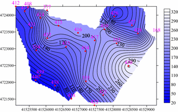
The contour of the thickness of coarse sandstone above the water flowing fractured zone at different borehole within the scope of the reservoir (unit: m)

5 Conclusions
-
1.
To evaluate the through degree of overlying strata fracture fissure induced by full mechanized mining and whether it spreads to the water under reservoir. Based on the drilling revealed stratum and the layout of working face in Daping mine field, The height of water flowing fractured zone of different workface on the outside of reservoir was the prediction sample, the comprehensive index weight value was determined by objective entropy method by selecting the measurable factors of the height of water flowing fractured zone of workface in Daping coal mine. The predictive value of the height of water flowing fractured zone near the borehole position within the scope of reservoir and the weights of all influencing factors was obtained by Matlab program. The inclined length of the working face and mining thickness were major factors on the height of water flowing fractured zone.
-
2.
The height of water flowing fractured zone of working faces within the scope of reservoir was about 150–200 m. The contours of the thickness of overlying layers and the different rock layers above water flowing fractured zone was obtained by Surfer software. And the safety evaluation of water-inrush was studied. The effective thickness of water-resisting layers above the height of water flowing fractured zone was the thinner at the location of Nos. 377, 438, 439, and 440 drilling hole. Therefore, we should choose rational mining method and the layout of working face. The scientific reference was provided for water prevention of mining working face and the layout of working face.
References
Chen PP, Liu HQ, Zhu ZX et al (2005) Height forecast of water conducted zone with top coal caving based on artificial neural network. J China Coal Soc 30(4):438–442 (in Chinese)
Cheng AB, Wang XM, Liu HQ (2011) Application of gray hierarchy analysis in the stability evaluation of underground mined-out areas. Metal Mine 2:17–20 (in Chinese)
Ding DX, Wang YG, Zhang ZJ (2005) Height research of water flowing fractured zone based on the adaptive neutral fuzzy inference. Min Technol 5(1):15–18 (in Chinese)
Gao XC, Wu YP (2011) Experimental study on dynamic distribution law of the spread cracks overlying stratum with rich water in special hard thick seam. Saf Coal Mines 42(3):16–18 (in Chinese)
Hu XJ, Li WP, Cao DT et al (2012) Index of multiple factors and expected height of fully mechanized water flowing fractured zone. J China Coal Soc 37(4):613–620 (in Chinese)
Kang YH, Zhao KQ, Liu ZG (2009) Devastating laws of overlying strata with fissure under high hydraulic pressure. J China Coal Soc 34(6):721–725 (in Chinese)
Li JS, Li ZY (2012) Height analysis of water flowing fractured zone of a coal mine mining under large-scale water mass. Saf Coal Mines 43(12):190–192 (in Chinese)
Liang GL, Xu WY, Tan XL (2010) Application of extension theory based on entropy weight to rock quality evaluation. Rock Soil Mech 31(2):535–540 (in Chinese)
Lin HF, Li SG, Cheng LH (2010) Model experiment of evolution pattern of mining-induced fissure in overlying strata. J Xi An Univ Sci Technol 30(5):507–512 (in Chinese)
Luan YZ, Li JT, Ban XH (2010) Observational research on the height of water flowing fractured zone in repeated mining of short-distance coal seams. J Min Saf Eng 27(1):139–142 (in Chinese)
Ma ZW, Ye YC, Wang QH (2013) Study on the height of water flowing fractured zone in containing vanadium shale deposit. Metal Mine 4:142–146 (in Chinese)
Pan H (2009) Prediction of water-flowing fractured zone’s height in roof of coal based on neural trained by particle swarm. Sci Mosaic 3:6–8 (in Chinese)
Shi LQ, Xin HQ, Zhai PH et al (2012) Calculating the height of water flowing fracture zone in deep mining. J China Univ Ming Technol 41(1):37–41 (in Chinese)
Wang SM (2006) A brief review of the methods determining the height of permeable fracture zone. Hydrogeol Eng Geol 30(1):64–66 (in Chinese)
Wang XM, Ke YX, Yan DB (2012) Underground goaf risk evaluation based on entropy weight and matter element analysis. China Saf Sci J 22(6):71–78 (in Chinese)
Xu ZM, Sun YJ (2011) Height prediction of the water conducted zone for mining under reservoir. China Min Mag 17(3):99–102 (in Chinese)
Zhao DS, Chen F, Wang ZC (2011) The experimental study on the failure of soft overburden in mining of thick coal seam. J Guangxi Univ Nat Sci Ed 36(1):177–181 (in Chinese)
Acknowledgements
This work was supported by 2017 Key Technologies of Prevention and Control of Serious and Major Accidents in Safety Production (liaoning-0005-2017AQ) and the National Natural Science Foundation of China (51774199).
Author information
Authors and Affiliations
Corresponding author
Rights and permissions
About this article

Cite this article
Wang, Z., Wang, C. & Wang, Z. The Hazard Analysis of Water Inrush of Mining of Thick Coal Seam Under Reservoir Based on Entropy Weight Evaluation Method. Geotech Geol Eng 36, 3019–3028 (2018). https://doi.org/10.1007/s10706-018-0520-0
Received:
Accepted:
Published:
Issue Date:
DOI: https://doi.org/10.1007/s10706-018-0520-0