
Abstract
In this paper, we propose a novel process to optical character recognition (OCR) used in real environments, such as gas-meters and electricity-meters, where the quantity of noise is sometimes as large as the quantity of good signal. Our method combines two algorithms an artificial neural network on one hand, and the k-nearest neighbor as the confirmation algorithm. Our approach, unlike other OCR systems, it is based on the angles of the digits rather than on pixels. Some of the advantages of the proposed system are: insensitivity to the possible rotations of the digits, the possibility to work in different light and exposure conditions, the ability to deduct and use heuristics for character recognition. The experimental results point out that our method with moderate level of training epochs can produce a high accuracy of 99.3 % in recognizing the digits, proving that our system is very successful.
1 Introduction
Optical Character Recognition (OCR) is a method to locate and recognize handwritten, type written or printed text stored in an image, such as a jpeg or a gif image, and convert the text into a computer recognized form such as ASCII or unicode. OCR is a field of research in pattern recognition, artificial intelligence and computer vision and converts the pixel representation of a letter into its equivalent character representation.
OCR is mainly applied to companies from paper-intensive industry having large collection of paper forms and documents and facing complex images environment in the real world: degraded images, heavy-noise, picture distortion, low resolution, etc.
Despite the benefits of OCR, certain limitations do still exist. In particular, many OCR programs suffer from a tradeoff between speed and accuracy. Some programs are extremely accurate, but are slower as a result.
Therefore a large amount of research has been carried out over a long time for finding and improving OCR algorithms. Mori et al. presented a very good overview of the existing OCR systems in [15] to which Blue et al. added a very pertinent and valuable evaluation in [2]. Regarding digit recognition, LeCun et al. [12] have given an overview of the existing algorithms. LeCun et al. [4] used neural networks for handwritten digit recognition. Rabiner et al. [16] used Markov models for the same purpose and Lee [13] proposed a combination of k-nearest-neighbor, radial-basis function, and neural networks. Deformable templates have been used by Jain et al. [11].
1.1 Requirements specification
This article is based on our experience with a real-life application researched and developed for several European companies specializing in automation for energy providers.
Such companies need OCR systems which can work in harsh and real environments, such as gas-meters and electricity-meters. There are several problems with them: they are not uniformly illuminated along the day, they are not uniformly exposed within the same shot (some parts are in shade, while some are over-exposed), the quantity of noise is very high, there is no possibility to fully train a system for all types of gas-meters, etc.
In such conditions, a robust system is required, especially when the application is in a practical setting and used by large companies with thousands of subscribers.
The size and zoom of the images may vary as well as the font and the color of the digits. Figure 1 shows several such images.

Several images to be processed by the OCR system
In summary, the requirement is to recognize the digits from gas-meters and electricity-meters obtained from web cameras in real environments. If the digits are visible less than 50 % of their height, the result will be discarded. The region for each digit is selected manually.
Our proposed system consists of a photo camera installed in front of the gas- or energy-meters. At predefined periods of time, it takes a snapshot which is processed by the OCR Processor. It returns the number obtained after OCR-izing the image. The number is sent to a central server and stored in a database. Further actions can be taken in accordance: invoicing, checking the meter, etc.
2 The general algorithm
The flow of our proposed process for character recognition is depicted in Fig. 2.

The general process of character recognition
The image is acquired using web cameras mounted in front of the gas- or electricity-meters and is fed as an input to the OCR system, which enhances it, processes it and returns the values of two digits: the last one before the decimal point, respectively the first one afterwards.
The process of digit recognition consists of several stages:
-
image pre-processing which converts the color image to a monochrome one, prepared for further analysis.
-
image thinning and segmenting for converting the digit (with a width) to a segmented line. The angles between subsequent segments will be the input for both the neural network as well as for the confirmation algorithm.
-
digit recognition using a neural network returns the most probable value of the digit with a confidence. We cannot rely solely on these results, therefore the next step is required.
-
confirmation of the result using the k-nearest neighbor is the stage in which the value of the digit is computed with a completely different algorithm.
-
computation of the confidence: In most cases, the values of the two approached should coincide. However, in practice they are not always the same. Therefore, a principle for accepting either result is required.
2.1 Image pre-processing
The images display a wide range of colors. Therefore the first step is to convert them to monochrome images (containing various intensities of gray). After the conversion, the general contrast is improved by histogram equalization (for more details see [17]). Through this adjustment, the intensities can be better distributed on the histogram. This allows for areas of lower local contrast to gain a higher contrast without affecting the global contrast. Histogram equalization accomplishes this by effectively spreading out the most frequent intensity values. A related technique is the enhancement of the high frequency details (sharpening). And finally, an adaptive thresholding (see [19]) brings up the digit (along with some noise).
Furthermore the image is sharpened. What actually happens, however, is the emphasizing of the edges in the image and making them easier for the eye to pick out—while the visual effects make the image seem sharper, no new details are actually created.
The final pre-processing step is adaptive thresholding, used to segment an image by setting all pixels whose intensity values are above a threshold to a foreground value and all the remaining pixels to a background value.
After this stage, the image is ready for further specific processing.
2.2 Thinning and Segmenting
Quite often, due to the difference in light exposure, the noise is attached to the digit itself and cannot be removed, like in Fig. 3.

A quite common case when the noise cannot be set aside the digit itself
In this case, the quantity of noise is almost equal to the number of pixels representing the digit itself. Feeding any recognition system with such a distorted signal would fail priori. Therefore an approach to reduce the noise as much as possible was necessary. This approach is called thinning, which is the process of reducing the digit to a line and subsequently segmenting that line into segments of equal size. The main characteristic of the thinning process is the preservation of the length.
We have come up with a novel algorithm based on the center of mass of each region of the digit. This assures a thinning in only one step, preserving the ratio between the length and the width of the image. The algorithm is as follows:
-
1.
Choose a bordering pixel, preferably starting with the left-most and top-most one, but not necessarily.
-
2.
Build the smallest square neighboring matrix (NM), containing the selected pixel and not overlapping an existing neighboring matrix. Each cornering pixel of the NM must have at most one neighboring pixel (on X and Y directions, not on diagonal) not belonging to the NM.
-
3.
The mass center is computed for the NM. If the NM is 2×2 and fully white, any of the pixels may be the mass center.
-
4.
Replace NM with the pixel in the mass center.
-
5.
Repeat from step 1 until there are no more available pixels.
-
6.
Connect the mass centers by lines, resulting in a thinned image.
A specific example presenting how the algorithm works is shown in Fig. 4.

The processing of thinning a digit. The blue lines represent the NM’s. The red pixels are the mass centers
The approach is as follows (see Fig. 4):
-
1.
the starting pixel is selected as the left most one
-
2.
the neighboring matrices (NM’s) are the blue rectangles
-
3.
the mass centers are computed for each NM and are colored red
-
4.
NM’s are replaced by their mass centers
-
5.
the above steps are repeated until there are no more available pixels
-
6.
the mass centers are connected by lines (the green lines in Fig. 5)
Fig. 5 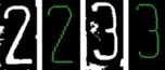
The source and the result of thinning and segmenting process for two digits: 2 and 3

The results of the proposed thinning and segmenting stage are depicted in Fig. 5.
Afterwards, the angles of the digit are computed. Those are the angles between each two adjacent segments.
Given the consecutive segments u and v, the angle made by them is computed as the angle between the vectors \(\overrightarrow{u}\) and \(\overrightarrow{v}\):
The angle between two 2D vectors is:
where ∥u∥ is the norm of the vector \(\overrightarrow{u}\), ⋅ is the cross product and arccos, the inverse of cosine function.
The first segment always starts from the top-most extreme point. That is the top-most point with only one neighbor. If there are n segments, then there will be n−1 angles. The last segment may or may not be adjacent to the first one. In other words, the first and the last point may coincide, like in the case of 0 and 8.
The algorithm has been developed in the following manner:
-
1.
Choose the first point as the top-most extreme point.
-
2.
Look at the adjacent point in the clockwise direction on the curve at a distance of k pixels. (In our experiments, k=5.)
-
3.
If the line has already been passed, look further clockwise (in other words “search on another line”). If there are other points, go to step 2.
-
4.
If there are no neighboring points, then stop.
-
5.
Repeat from step 2.
Depending on the digit, the number of segments may vary significantly. The shortest digits are 1 and 7, the longest one is 8. However, there is no limit imposed to the number of segments.
The accuracy of the classification has been computed in the following cases:
-
1.
Using pre-processed digits, with no further improvements
-
2.
Using thinned digits
-
3.
Using the angles of the digits (after thinning)
The results are depicted in Fig. 6.

Accuracy rate after using pre-processed digits, using thinned digits, respectively using also the angles of the digits
2.3 OCR by neural network
A neural network (NN) involves a network of simple processing elements (artificial neurons) which can exhibit complex global behavior, determined by the connections between the processing elements and element parameters. Artificial neurons were first proposed in 1943 by Warren McCulloch, a neurophysiologist, and Walter Pitts, an MIT logician [14], but NN became sophisticated enough for applications at the middle of 1980’s.
In a neural network model simple nodes, which can be called variously “neurons”, are connected together to form a network of nodes, hence the term “neural network”. The nodes are arranged in a way that each node derives its input from one or more nodes and are linked through weighted connections. While a neural network does not have to be adaptive in itself, its practical use comes with algorithms designed to alter the strength (weights) of the connections in the network to produce a desired signal flow.
There are many algorithms for training neural networks; most of them can be viewed as a straightforward application of optimization theory and statistical estimation. They include: back propagation by gradient descent, conjugate gradient, and resilient back-propagation ([5, 18]). Evolutionary computation methods, simulated annealing, expectation maximization and non-parametric methods are among other commonly used methods for training neural networks.
Some of the advantages of the NN are: the ability to recover from distortions in the input data, the capability of learning and the insensibility to noise. Because of their parallel architecture, high computational rates are achieved as well.
In our case, the input of the neural network consists of the angles between subsequent segments as computed in Eq. (2). This approach has several advantages over the algorithms using the value of each pixel:
-
the input is significantly smaller,
-
the weight of the noise is reduced,
-
the rotation of the digits does not affect the neural network architecture and its inputs.
Our considered neural network is a multi-layer perceptron (MLP): the first layer connects the input variables and is called the input layer, the last layer connects the output variables and is called output layer and the layer between the input and output layers is called hidden layer. The input layer consists of 35 rows, which is the highest number of angles. The hidden layer consists of 15 units. The output layer consists of 10 units, one for each digit.
Transfer functions of a neuron, in neural networks, calculate a layer’s output from its net input and are chosen in such a way to have a number of properties which enhance or simplify the network containing the neuron. In our approach, we used two different transfer functions, for the hidden and output layer:
-
the softMax transfer function (for the output layer), defined as:
$$ f(x_i) = \frac{e^{x_i^{lin}}}{\sum_j{e^{x_j^{lin}}}} $$(3)where \(x_{i}^{lin} = \beta x_{i}\), with β being the scaling factor and x i the input of the node.
This function is usually utilized on the output layer when the results need to be interpreted as a probability. This means that the sum of all outputs is 1 and the signal of a node is the probability that an image is the digit associated to that node.
-
the hyperbolic tangent sigmoid transfer function (for the hidden layer), is defined as
$$ \mathrm{tanh}(u) = \frac{2}{1+e^{-2u}} -1 $$(4)where the total synaptic input u to the neuron is given by the inner product of the input and weight vectors:
$$u = \sum w_i x_i + b_i \;. $$
The learning rule has a huge influence upon the neural performance. The training must be quite fast and not make the network over-fit the training set. In our approach, we used the Fahlman’s quickprop algorithm (see [9]) as a learning rule. This algorithm is a gradient search procedure that has been shown to be very fast in a multitude of problems. It basically uses information about the second order derivative of the performance surface to accelerate the search. The number of epochs was set to 500. Over this number, the neural network becomes over-trained, meaning that it classifies the digits in the training set very well, but performs poorly on new inputs. This decision was made based on the results described in Table 1, where the column Time shows the time needed for the training, column Training Cost shows the cost (error) of the training, whereas the CV Cost shows the cost of the network performing on the cross-validation set.
A set of images is used for training and another set for cross-validation. The cross-validation is used for checking how the neural network performs on a new input set. If the network is overtrained, it performs very well on the training set and very bad on the cross-validation set. There are two modes of learning to choose from: one is on-line (incremental) learning and the other is batch learning. In on-line learning, each propagation is followed immediately by a weight update. In batch learning, many propagations occur before weight updating occurs. Batch learning requires more memory capacity, but on-line learning requires more updates.
The training set consists of the segmented images from 2 gas- and electricity-meters taken with web cameras in real conditions. Back-propagation neural networks have been used for training the network.
After training, the network was tested on the images from the other 3 gas-meters and electricity-meters.
OCR errors can be modeled statistically and are very different from human mistakes. Confusion matrix models these errors in order to be able to correct them and to improve the OCR.
The confusion matrix, based on the classification of the neural network, in the case of the considered transfer functions for the output layer are shown in Tables 2 and 3.
Table 2 states that 0 was classified correctly in 90 % of the trials and as 8 in 10 % of the cases. The least correctly classified digit was 3, which was mistaken for 0 in 20 % of the cases, for 4 in 5 % and for 8 in 10 % of the trials. Digit 6 was classified correctly for all the experiments. This table gives a clear idea about the similarities between various digits, such as 0, 3, 8 and 9 on one hand, respectively 1 and 7 on the other hand.
Analyzing the results presented in Table 3, we observe that the best recognized characters are 0, 2 and 7. Digits 1, 3, 4, 5, 6, 8 and 9 are recognized with the accuracy below 65 %. Character 1 is confused mostly with 7, digit 3 is mistaken mostly for 0 and 8, digit 4 is mistaken mostly for 2, 5 is confused with 6 and 8 is confused mostly with 9.
Analyzing the results presented in Tables 2 and 3, we observe that a higher accuracy rate was obtained in the case of the softMax function. This is the main reason for choosing this as a transfer function.
2.4 Confirmation by k-nearest neighbor
For confirmation of the result of the neural network, the k-nearest neighbor (k-NN) algorithm has been used.
The nearest neighbor (k-NN) is a well-known approach used to classify characters ([3]) and predictions’ ([10]). The distance measured between the two characters images is needed in order to use this rule. The rule involves a training set of positive and negative cases and a new sample is classified by calculating the distance to the nearest one.
When the amount of the pre-classified points is large, it is good to use a majority vote of the nearest k neighbors instead of the single nearest neighbor. This method is called the k nearest neighbor (k-NN).
The k-nearest neighbor algorithm is among the simplest of all machine learning algorithms. An object is classified by a majority vote of its neighbors, with the object being assigned to the class most common among its k nearest neighbors.
The same method can be used for regression, by simply assigning the property value for the object to be the average of the values of its k-nearest neighbors. It can be useful to weigh the contributions of the neighbors, so that the nearer neighbors contribute more to the average than the more distant ones.
The neighbors are taken from a set of objects for which the correct classification (or, in the case of regression, the value of the property) is known. This can be thought of as the training set for the algorithm, though no explicit training step is required. In order to identify neighbors, the objects are represented by position vectors in a multidimensional feature space. It is usual to use the Euclidean distance. However, as the objects are made of angles, we simply used the distance between angles, that is the absolute value of their difference. The k-nearest neighbor algorithm is sensitive to the local structure of the data.
An object (digit) is a vector consisting of the angles computed as in Sect. 2.2 along with their number:
The distance between two objects:
is given by
where |a| is the absolute value of a.
If two objects are of different length, the shorter one is filled with null values until the lengths of the two objects are equal.
After the confirmation step using the k-NN algorithm, the confusion matrix looks like in Table 4.
From Table 4 we can see that digit 1 was still mistaken for 7 and 9, digit 4 for 1 and 6, and digit 8 for 9 and vice versa. However, the percentages of misclassified trials is significantly lower than after the first step, using the neural network (see Sect. 2.3).
2.5 Confidence computation
In addition to the quantitative results, we also analyzed our results qualitatively.
Both algorithms used in our process for OCR return a result with some confidence, which is different than 100 % in most cases. When the confidence factors are high or when the results of the two approaches are the same, the result is straightforward and requires no further discussions.
For the OCR by neural network, the confidence factor CF NN is the probability returned on the output layer by the softMax function.
For the OCT by k-NN, the confidence factor is computed as following. Let d i be the distance from the digit to the recognized number i. Defining the inverse distance as \(id = \frac{1}{d_{i}}\), the global inverse distance is \(\mathit{ID} = \sum_{i = 0}^{9}{id}\).
The probability that a given image represents the number i is \(P_{i} = \frac{id}{\mathit{ID}}\), which is also the confidence factor CF kNN that an image represents a number based on the k-NN algorithm.
The algorithm of deciding upon the result of the process is described in Algorithm 1.

The confidence computation algorithm
The problems occur when the confidence factors are low and the results differ. In this case, the final result (output digit) is selected based on some heuristics. In our experiments, we considered the following heuristics:
-
the length of a digit:
-
short digits are those digits whose length is less than 20 segments. These are 1 and 7.
-
medium-sized digits are the ones consisting of more than 20 segments, but less than 35. These are 2, 3, 4, 5.
-
long digits are the ones longer than 35 segments, such as: 0, 6, 8 and 9.
-
-
the position of the last segment relatively to the first one
-
adjacent segments for digits 0 and 8;
-
non-adjacent segments for all the other digits.
-
-
characteristics of the curve (open of closed, intersecting or free etc.)
-
open curve is characteristic to the digits 1, 2, 3, 5, 7.
-
completely closed curve is the curve for each the first and the last pixel coincide and it is specific to 0 and 8.
-
partially closed curve is specific to 6 and 8. Digits 4 may have or not a closed curve, depending on the font.
-
The first important observation is that the total “length” of a digit gives a significant clue about its value. The “length” of a digit is the number of segments which cover it entirely.
Such a classification is important for several reasons:
-
it brings another tool to digits analysis;
-
it can be the starting point of an OCR based on decision trees;
-
it can also be the starting point of an OCR knowledge-based.
The confusion matrix after the confidence computation is presented in Table 5.
As can be seen from Table 5, the accuracy of the process increases significantly after the confidence computation. The minimum accuracy is 98 % for digits 3 and 8, which are mistaken for each other sometimes. The accuracy for the whole test set is 99.3 %.
The accuracy of the proposed process after each classification step (using the neural network, using the k-nearest neighbor, respectively after the confidence computation) is shown in the Fig. 7. The x-axis values represent the digits and the y-axis values are the accuracy rates for each digit.

Accuracy rate after NN classification, k-NN classification and confidence computation
3 Comparative results
Because in the case of real environments, we did not find any other OCR methods, in order to prove the performance of our proposed approach, we test it against the images of NIST Special Database 3 [6].
According to Guyon et al. [7], the NIST data set SD3 contains one of the largest selections of isolated digits and characters that are publically available. Altogether it contains 223,124 character images that were extracted from data collection forms filled out by 2100 individuals. Employees of the U.S. Bureau of the Census were instructed to fill the boxes on a form with a particular sequence of digits or characters and were asked to make sure that the individual digits or characters did not touch one another or the surrounding box. The forms were subsequently scanned at 300 dpi in binary mode and automatically segmented. The string of digits that should have been written in each box were used to assign a truth value to each individual image. The truth values were subsequently verified by a human operator.
We have compared the results obtained using our proposed approach with the ones reported by Atukorale et al. [1] and Ha et al. [8]. Atukorale et al. partitioned the dataset into three non-overlapping sets with 106,152 samples for training, 53,076 for validation, and 63,896 for testing. We have opted for the approach described by Ha et al., who partitioned the images into 40,000 samples for training, 10,000 for validation and 173,124 for testing.
The HONG network developed by Atukorale et al. obtained a recognition rate of 99.59 % while the system proposed by Ha et al. based on a perturbation method obtained an accuracy of 99.54 %. Our developed process reached an accuracy of 99.58 %, better than the system proposed by Ha et al. [8] and very close to method described by Atukorale et al. [1].
The robustness of our approach is given by the fact that each recognition is done by two different algorithms - a neural network approach and a k-nearest neighbor algorithm. If the recognized character is the same in both cases, then the confidence of the result is high. Otherwise, some heuristics are used within the step confidence computation. The former two algorithms are very mathematical and objective, whereas the latter one is rather subjective. It applies a completely different approach to make a clear distinction between the characters returned by the previous algorithms if they have different results. The heuristics used refer to the features of digits, such as length, shapes, curves etc.
4 Conclusions
Using a neural network approach, back-propagation for learning and the k-nearest neighbor for confirmation of digit recognition in noisy environments was very successful. The accuracy rate of recognizing the numbers was 99.3 %. This accuracy rate is very high and we can conclude that the overall recognition system was successful.
Our proposed process was tested on real-life pictures highly distorted from gas- and electricity-meters. No noise was added manually for the sake of experiments, a complete training set was not available since the range of the tools used for various energy measurements was very wide, with no standards regarding the fonts, colors and sizes.
An important feature of our novel approach to digit recognition in real environments is that it is based on the angles of the digit, rather than the values of the pixels in the image and therefore it is insensitive to the digit rotation. Although it has been applied specifically to digit recognition, it can be extended for any character recognition. Its main strength is the robustness to noise, quite common in real-life applications, where the distortion can be up to 50 %.
From the experimental results, we observe that our proposed approach has trouble identifying the digit 3. This is probably caused by the fact that it looks like digits 8 and 0.
In conclusion, our proposed approach has several advantages, such as: insensitivity to the possible rotations of the digits, the possibility to work in different light and exposure conditions, the ability to deduct and use heuristics for character recognition. These make it very good for real life applications, such as OCR of the gas- and electricity-meters.
Future research will be dedicated to combining pixel-based approaches with the angle-based method proposed in order to improve the results.
References
Atukorale AS, Suganthan PN, Downs T (2000) On the performance of the HONG network for pattern classification. In: Proceedings of the IEEE-INNS-ENNS international joint conference on neural networks, vol 2, pp 285–290
Blue JL, Candela GT, Grother PJ, Chellappa R, Wilson CL (2004) Evaluation of pattern classifiers for fingerprint and ocr applications. Pattern Recognit 27(4):485–501
Boiman O, Shechtman E, Irani M (2008) In defense of nearest-neighbor based image classification. In: IEEE conference on computer vision and pattern recognition, pp 1–8
Le Cun Y, Boser B, Denker JS, Howard RE, Habbard W, Jackel LD, Henderson D (1990) Handwritten digit recognition with a back-propagation network. Adv Neural Inf Process Syst 2:396–404
Garcez ASA, Zaverucha G (1999) The connectionist inductive learning and logic programming system. Appl Intell 11(1):59–77
Garris MD, Wilkinson RA (1992) Handwritten segmented characters database. Technical report special database NIST 3, February 1992
Guyon I, Haralick MR, Hull JJ, Phillips TT (1997) Data sets for OCR and document image understanding research. In: Handbook of character recognition and document image analysis, pp 779–799
Ha TM, Bunke H (1997) Off-line, handwritten numeral recognition by perturbation method. IEEE Trans Pattern Anal Mach Intell 19(5):535–539
Hoehfeld M, Fahlman SE (1995) Learning with limited numerical precision using the cascade-correlation algorithm. IEEE Trans Neural Netw 3(4):602–611
Huang C-C, Lee H-M (2004) A grey-based nearest neighbor approach for missing attribute value prediction. Appl Intell 3(20):239–252
Jain AK, Zongker D (1997) Representation and recognition of handwritten digits using deformable templates. IEEE Trans Pattern Anal Mach Intell 19(12):1386–1390
Le Cun Y, Jackel L, Bottou L, Brunot A, Cortes C, Denker J, Drucker H, Guyon I, Muller U, Sackinger E, Simard P, Vapnik V (2004) Comparison of learning algorithms for handwritten digit recognition. In: Proceedings of the international conference on artificial neural networks, pp 53–60
Lee Y (1991) Handwritten digit recognition using k nearest-neighbor, radial-basis function, and back-propagation neural networks. Neural Comput 3(3):440–449
McCulloch WS, Pitts W (1943) A logical calculus of the ideas immanent in nervous activity. Bull Math Biophys 5:115–133
Mori S, Suen CY, Yamamoto K (1992) Historical review of ocr research and development. In: Proceedings of IEEE, special issue on OCR, pp 1029–1075
Rabiner LR, Wilpon JG, Soong FK (1999) High performance connected digit recognition using hidden Markov models. IEEE Trans Acoust Speech Signal Process 37(8):1214–1225
Russ JC (2011) The image processing handbook. CRC Press, Boca Raton
Schaal S, Atkeson CG, Vijayakumar S (2002) Scalable techniques from nonparametric statistics for real time robot learning. Appl Intell 17(1):49–60
Shapiro LG, Stockman GC (2002) Computer vision. Prentice Hall, New Jersey
Acknowledgements
This work was supported by a grant of the Romanian National Authority for Scientific Research, CNCS-UEFISCDI, project number PN-II-RU-TE-2011-3-0113.
Author information
Authors and Affiliations
Corresponding author
Rights and permissions
About this article
Cite this article
Matei, O., Pop, P.C. & Vălean, H. Optical character recognition in real environments using neural networks and k-nearest neighbor. Appl Intell 39, 739–748 (2013). https://doi.org/10.1007/s10489-013-0456-2
Published:
Issue Date:
DOI: https://doi.org/10.1007/s10489-013-0456-2