A survey on skin detection in colored images

Abstract

Color is an efficient feature for object detection as it has the advantage of being invariant to changes in scaling, rotation, and partial occlusion. Skin color detection is an essential required step in various applications related to computer vision. The rapidly-growing research in human skin detection is based on the premise that information about individuals, intent, mode, and image contents can be extracted from colored images, and computers can then respond in an appropriate manner. Detecting human skin in complex images has proven to be a challenging problem because skin color can vary dramatically in its appearance due to many factors such as illumination, race, aging, imaging conditions, and complex background. However, many methods have been developed to deal with skin detection problem in color images. The purpose of this study is to provide an up-to-date survey on skin color modeling and detection methods. We also discuss relevant issues such as color spaces, cost and risks, databases, testing, and benchmarking. After investigating these methods and identifying their strengths and limitations, we conclude with several implications for future direction.

1 Introduction

In order to analyze, interpret, or understand an image automatically, the pixels that belong to a particular object of interest need to be identified unambiguously. The process of such identification is known as segmentation (Efford 2000). Formally, segmentation subdivides an image into its constituents or objects (Gonzalez and Woods 2002). Cheng et al. (2001) defined image segmentation as “the process of dividing an image into different regions such that each region is homogeneous, while the union of any two adjacent regions is not”. Fu and Mui (1981) defined image segmentation as “the division of an image into different regions, whereby each region has certain properties”. From our point of view, the aim of segmentation is to group together pixels that have similar properties, according to a set of predefined criteria, and as a result divides the source image into a set of regions that represent different objects. The regions of pixels that we generate should be meaningful. The level to which the subdivision is carried depends on the problem being treated (Guru et al. 2010). The segmentation task is divided into two types: complete and partial image segmentation (Sonka et al. 2008):

• i. Complete image segmentation Results in a set of disjoint regions corresponding to objects in the source image. Hence, it can be formulated as follows: Let R represent the entire image region. Segmentation can be viewed as a process that partitions R into n sub-regions R₁, R₂, R₃, ….R_n such that:

  $$ \mathop {\bigcup }\limits_{i = 1}^{n} \,R_{i} = R; $$

  (1)

  and

  $$ {\text{R}}_{\text{i}} \cap {\text{R}}_{\text{j}} = \emptyset \,{\text{for all}}\,i\,{\text{and}}\,j, {\text{where}}\, {\text{i}} \ne {\text{j}} $$

  (2)

  The first condition implies that every image pixel must be in a region. This means that the segmentation algorithm should not terminate until every pixel is processed. The second condition means that no pixel can belong to more than one region. However, an individual pixel cannot indicate whether it is located in a region. Hence the neighborhood of the pixel needs to be analyzed. If the pixel shows the same properties as its neighbors, then we have a good reason to believe that it lies within a region of similar values.

• ii. Partial image segmentation A reasonable aim of many image processing and vision applications is to apply partial segmentation with respect to a chosen property such as brightness, color, texture, etc. So, partial segmentation should stop when the regions of interest are isolated. Typically, the output of partial segmentation will be a binary image where the regions of interest (e.g., objects) are set to 1’s while a background pixel is given a value of “0” (i.e., excluding background regions). This would reduce the size of data to be processed. The substantial reduction in data volume offers an immediate gain, which is important to most applications. Skin detection problem falls in this category of image segmentation.

The skin detection is the process of segmenting the input image into skin and non-skin regions (i.e., identifying skin pixels). By skin regions, we mean any exposed part of the human body that appears in the image such as faces, shoulders, hands, legs, etc. Evidently, skin detection is the first step in many automated systems associated with image processing applications such as face detection/recognition (Zaqout et al. 2004; Xiaohua et al. 2009; Verma et al. 2014; Pujol et al. 2017; Kovac et al. 2003; Hsu et al. 2002), video surveillance systems (Gejguš and Šperka 2003; Kim et al. 2005; Barbu 2014; Chaichulee et al. 2017), naked image detection (Perez et al. 2017; Carlsson et al. 2008; Duan et al. 2002; Rowley et al. 2006; Lee et al. 2007; Sevimli et al. 2010; Chin 2008), content based image retrieval (Albiol et al. 2000; Ma and Zhang 1999), and hand gesture recognition (Yang 2000; Habili et al. 2004; Ruijsscher 2006; Bretzner et al. 2002; Chen et al. 2003; Jalab and Omer 2015; Rautaray and Agrawal 2015).

Our goal, in this study is to provide an up-to-date survey on the current techniques related to skin detection problem. We tried to summarize the most notable and significant differences between these techniques, their strengths and limitations and characteristic features.

The remainder of the study is organized as follows: Sect. 2 gives a brief description of image segmentation based on skin color. In Sect. 3, we will discuss the challenges associated with of skin segmentation problem. The properties of human skin are described in Sect. 4. Section 5 describes costs and risks of classification errors. Color spaces, reducing the dimensionality of color spaces, and comparison between color spaces are descripted in Sects. 6, 7, 8 respectively. In Sect. 9, we give a detailed review of methods to detect human skin in a single image. Benchmarking databases and evaluation criteria are discussed in Sects. 10 and 11 respectively. Conclusion is presented in Sect. 12.

2 Image segmentation based on skin color

From the point of segmentation bases, Gonzalez and woods (2002) classified segmentation algorithms into two basic categories: discontinuity and similarity. In the first category, the approach is to partition an image based on abrupt changes in intensity, such as point detection, edge detection, and boundary detection. The principal approaches in the second category are based on partitioning an image into regions that are similar according to a set of predefined criteria. Pixel-based segmentation, region-based segmentation, region splitting and merging, and watershed segmentation algorithms are examples of methods in this category.

Segmentation algorithms can be done interactively or automatically. Suitable and excellent segmentation methodologies are usually interactive, that is, under control of users; partition the image into non-overlapping regions of interest. Automatic image segmentation algorithms might be required for most of the vision-based systems and it would be ideal for automatic object detection. Efford (2000) stated that a reliable and accurate image segmentation is generally very difficult to achieve by purely automatic means.

Since image segmentation is the first step in image analysis, the accuracy of segmentation determines the eventual success or failure of computerized system. For this reason, considerable care should be taken to improve segmentation accuracy.

Until recently many of the object detection methods such as PCA, ANN, SVM, HMM, etc., were done at the intensity level using gray scale images. The segmentation of gray images is a very difficult task as in general, intensity information does not provide enough information as color images. Therefore, most of these methods are based on appearance-based approaches that imply high computational cost as well as high false detections (Roth and Winter 2008). Therefore, it is needed to process local information in a very short period of time in order to identify “hot spots” (or “regions of interest”) which are likely, though not certain, to contain a desired object or class of objects (e.g., human face). Then, more complex classifier that usually requires intensive high processing are used to make the final arbitration of whether these “hot spots” correspond to objects of interest or not.

The use of color as a valuable feature in image analysis is motivated by the following principal factors:

• (1) Color images can provide more information than gray level images (Shapiro and Stockman 2001; Russ 2007). Often, when the objects cannot be extracted using gray scale, they may be easily extracted using color information. For example, two objects of similar gray tones might be very different in color. Hence color is a powerful feature that often simplifies object detection and extraction from a scene (Gonzalez et al. 2007).

• (2) Color is robust against object rotation, scaling, and partial occlusion.

• (3) The processing of color information has proven to be much faster than processing of some other features (Gonzalez et al. 2007).

• (4) The background in complex images usually contains objects and patterns that look like similar to targeted object. An advantage of skin color segmentation is to reduce the probability of false detections which improves the accuracy of the system (i.e., excluding the background). We will show in the subsequent sections that most of the colors (i.e., about 90.36%) in the color set are non-skin colors.

• (5) Color information can be combined with other complementary features. This will help achieving better detection rate.

3 Challenges of skin color detection

With diversity of image types and sources, human skin color can vary dramatically in its appearance that makes accurate skin detection a challenging task. The challenges associated with skin detection can be attributed to the following factors:

• Illumination variations In real world cases, the illumination variation is the most important problem that seriously degrades the segmentation performance (Storring 2004). A change in the light source distribution or in the illumination level (indoor, outdoor, highlights, shadows, non-white lights) produces a change in the color of the skin. Usually, the dark shadow on the face is a result of strong directional lighting that has partially blackened some facial regions. This is due to the non-plane shape of the facial features. Sometimes, a face has a “bright spot” due to reflection of strong lighting.

• Different ethnic groups (Race) Skin color appearance varies from person to person due to physical differences among human racial groups. For example, Europeans (Caucasians), Africans, Asians, etc. have different skin colors that range from white, to brown to dark (Tan et al. 2012).

• Imaging conditions When the image is formed, factors such as camera characteristics (sensor response, lenses) affect the skin appearance. In general, different color cameras do not necessarily produce the same color appearances for the same scene under the same imaging conditions (Yang et al. 2002).

• Image montage and reproduction Different image collections from the internet, movies, newspapers, and scanned images are usually uncontrollable and have virtually unlimited sort of montage processes. There are tools to reproduce skin tones including setting new pigment concentration and changing the color of skin image by applying color transfer technology. Some images already have been captured with the use of color filters. This makes dealing with color information even more difficult.

• Makeup Affects the appearance of skin color (Kakumanu et al. 2007).

• Aging Human skin varies from fresh and elastic skin to dry rough skin with wrinkles.

• Complex background Is another challenge that comes from the fact that many objects in the real world might have skin-like color. For example, furniture, clothes, blond hair, rocks, etc. The diversity of backgrounds is virtually unlimited. This causes the skin detector to produce false detections (Kakumanu et al. 2007).

When developing a system that uses color information as a cue feature, the researchers have to deal with three main sub-problems (Vezhnevets et al. 2003): First, what color space to choose for skin segmentation in relation to a certain application? Second, how to build a skin model that represents skin color distribution in the color space? And finally, what will be the method of image segmentation? These sub-problems will be discussed in detail in the subsequent sections.

4 Properties of human skin

Skin color appearance gives us a sign about the person’s race, mode, healthy, and the age. Human skin consists of three main layers (i.e., epidermis, dermis and subcutaneous) (Martinkauppi 2002). Each has its function and all skin layers work together. The outer surface of skin is covered with dead cells causing no regular reflection, while the glossiness of skin can be because of sweat or skin oil.

Complex phenomena can happen during the interactions between incident light and skin (Storring 2004). The final skin spectra are formed by the interaction between skin and light: light striking skin is transmitted, absorbed, and reflected through the layers. The spectra for human skin generally form a continuous homologous series because of characterization caused by absorption of melanin and hemoglobin, in which melanin in epidermis and hemoglobin in dermis play dominant roles and mostly decide the skin appearance (Martinkauppi 2002).

5 Costs and risks

Skin segmentation may cause two kinds of classification errors: False Negative errors (FNs) in which a skin pixel is classified as a non-skin pixel, and False Positive errors (FPs) in which an image pixel is classified as skin pixel, although it is not (Zainuddin et al. 2010). In general, complex backgrounds usually increase FPs errors due to the fact that natural scenes contain many objects with skin-like colors. On the other hand, variations in illumination, ethnic groups, and camera characteristics usually increase FNs errors. We should realize that classification errors are rarely avoided even for an ideal application. Moreover, it is generally accepted that each type of classification error has an associated cost or risk. It is possible to assume that the consequences of classification errors are equally costly. For example, classifying a novel pixel as a non-skin when in fact it is skin, is just like the cost of the converse (i.e., classifying a pixel as a skin when in fact it is non-skin). Unfortunately, most researchers in the field assumed equal misclassification costs. In real-world problems, such symmetry in the cost is problematic due to the fact that the classification error of one type is much more expensive than another.

In relation to skin segmentation problem, the cost of FNs rate is more expensive than FPs rate, attributed to the fact that image segmentation is the first step in image analysis of many systems. When a skin region is misclassified (i.e., skin region labeled as background), the system’s subsequent steps cannot retrieve it back. In contrast, FPs errors can be eliminated later due to the fact that it is expected that the detected skin-tone regions will include some non-skin regions whose color is similar to skin-tone. The system’s subsequent steps can make the final arbitration and reject these ‘skin-tone’ regions that do not belong to human body (i.e., validate the segmentation results). Therefore, researchers should design their classifiers in such a way that it minimizes the total expected cost (Duda et al. 2001).

6 Color spaces used for skin detection

Color is not an intrinsic property of an object itself. It is the perception of the energy emitted or reflected from it. When light hits objects, some wavelengths are absorbed and some are reflected, depending on the object materials. The reflected wavelengths are perceived (i.e., by the eye’s light receptor cells) as the object’s color (Gonzalez and Woods 2002).

In computer vision, digital imaging works by transforming colors into numbers either by using the physics of light waves, or the way the eye perceives color, or the way ink creates colors. The model that represents these numbers is called the color model or color space. The color space is a mathematical model to represent and visualize colors as tuples of numbers, typically as three or four values of color components (or channels). The color space represents a coordinate system where each specific color is represented by a single point in the coordinate system. The various color spaces exist because they present color information in ways that make certain calculations more convenient or because they provide a way to identify colors that is more intuitive (Russ 2007; Sonka et al. 2008).

In the field of skin detection, the most widely used color spaces are classified as follows (Russ 2007; Kakumanu et al. 2007):

• Basic color spaces (RGB, Normalized RGB);

• Perceptual color spaces (HSI, HSV, HSL, TSL);

• Orthogonal color spaces (YCbCr, YIQ, YUV, YES);

• Perceptually uniform color spaces (CIE-Lab, CIE-XYZ and CIE-Luv);

• Others color ratio space (IUV), mixture spaces.

Many users, digital cameras, color monitors, and other storage devices employ the RGB model as the default color space to display and store digital images. However, some applications may find it more convenient to use other color spaces. To cope with the skin detection challenges, many researchers have focused on selecting the most suitable color space for skin detection (Vezhnevets et al. 2003; Kakumanu et al. 2007; Chaves-González et al. 2010). For example, Fig. 1 shows color representation in four different color spaces; RGB, HSV, CIE lab, and YUV. Figure 2, adopted from (Nadian-Ghomsheh 2016), shows skin color distribution using different color spaces, these are RGB, normalized RGB, CbCr, and HS spaces that obtained from the skin pixels in the training dataset.

Fig. 1

Color representation in different color models; a RGB color space; b HSV color space; c CIE chromate color space; d YUV color space. (Color figure online)

Fig. 2

Skin color distribution using different color spaces, adopted from Nadian-Ghomsheh (2016); a Skin color distribution in RGB color space; b Skin color distribution in normalize RGB color space; c Skin color distribution in CbCr chromaticity space; d Skin color distribution in Hue-Saturation chromaticity space. (Color figure online)

6.1 RGB and normalized RGB color spaces

RGB model is based on the Cartesian coordinate, where each color is represented in its three primary components: Red (R), Green (G), and Blue (B). It can be geometrically represented in a three-dimensional cube with three axes perpendicular to each other as shown in Fig. 1a. The RGB color model is implemented in different ways, depending on the capabilities of the system used. The most common system used is an 8-bit per one component to describe a color, resulting in the 24-bit implementation (i.e., the number of bits required to represent a pixel in a colored image). Any color space based on such a 24-bit model is thus limited to a range of 256 × 256 × 256 ≈ 16.7 million colors (Ma and Leijon 2010). Some implementations use more bits per component (e.g., 16 bits), resulting in a larger number of distinct colors.

Since the RGB model is the most commonly used in digital images, we have to enlighten the main properties of this model (Ma and Leijon 2010; Gonzalez and Woods 2002; Russ 2007; Sonka et al. 2008):

• Different colors are defined by combinations of Red, Green, and Blue primary color components. These primary colors are at the corners (255,0,0), (0,255,0), and (0,0,255); black is at origin (0,0,0) and white at the opposite corner (255,255,255). The different colors in the RGB model are points on or inside the cube, see Fig. 1a.

• The diagonal line of the cube is from black (0,0,0) to white (255,255,255), representing all the gray levels, in which, the three components R, G, and B are the same.

• The RGB color space is an “additive” model as in nontechnical terms, its origin starts at black, and all other colors are derived by adding intensity values.

• The RGB cube is smaller than our visible range and represents fewer colors than what we can see (Burdick 1997).

• The RGB colored image of screen dimension M rows and N columns is an M × N × 3 of colored pixels. Here, 3 represents the three layers of Red, Green, and Blue intensities.

• Although RGB is suitable for technical applications, it is of limited use (not preferable) for image segmentation because of the high correlation between the R, G, and B components. It is not a perceptual model (Efford 2000); that is, the R, G, and B components contain both the color (chrominance) and luminance (intensity) information.

• The main advantage of the RGB space is its simplicity.

• Conversion from RGB to the other color spaces is straightforward and loses no information except for possible round-off errors (Russ 2007).

The transformation of RGB to normalized RGB can be obtained by the process of normalization.

$$ R_{n} = \frac{R}{{\left( {R + G + B} \right)}} $$

(3)

$$ G_{n} = \frac{G}{{\left( {R + G + B} \right)}} $$

(4)

$$ B_{n} = \frac{B}{{\left( {R + G + B} \right)}} $$

(5)

The component B_n can be omitted because it does not hold any significant information (i.e., it is known that R_n+ G_n+ B_n = 1). Thus, reducing the space dimensionality is preferable. Due to their popularity, the RGB and normalized RGB color spaces were used for skin color modelling and detection by Bergasa et al. (2000), Oliver et al. (2000), Greenspan et al. (2001), Chen and Wang (2007), Sebe et al. (2004), Seow et al. (2003), Storring et al. (2003), Kovac et al. (2003), Jones and Rehg (2002), Siddiqui and Wasif (2015), Khan et al. (2014a) and Hajraoui and Sabri (2014).

6.2 YUV color space

Previous black-and-white TV systems used only (Y) information. The Y component, (luminance or luma) determines the brightness of a monochrome image that would be displayed by a black-and-white television receiver. Engineers needed a signal transmission method that was compatible with black-and-white TV while being able to add color. Color information (U and V) was added separately so that a black-and-white receiver would still be able to receive and display a color picture transmission in the receiver’s native black-and-white format. The YUV color model is used in the PAL and SECAM color TV broadcasting. Y ranges from 0 to 1 (or 0–255 in digital formats), while U and V range from − 0.5 to 0.5, (or − 128 to 127 in signed digital form, or 0 to 255 in unsigned form) as shown in Fig. 1d. For 8-bit (256 value) image, the transformation of RGB to YUV color space is as follows (Russ 2007):

$$ \left[ {\begin{array}{*{20}c} Y \\ U \\ V \\ \end{array} } \right] = \left[ {\begin{array}{*{20}c} 0 \\ {128} \\ {128} \\ \end{array} } \right] + \left[ {\begin{array}{*{20}c} {0.299} & {0.587} & {0.114} \\ { - 0.169} & { - 0.331} & {0.500} \\ {0.500} & { - 0.418} & { - 0.081} \\ \end{array} } \right]\left[ {\begin{array}{*{20}c} R \\ G \\ B \\ \end{array} } \right] $$

(6)

This color space was used for skin color modelling and detection by Li et al. (2007) and Vadakkepat et al. (2008).

6.3 YIQ color space

YIQ was formerly used in the National Television Systems Committee (NTSC) television (North America, Japan, Thailand, Korea). NTSC defines a color space known as YIQ which is similar to the YUV model. The YIQ and YUV stem from broadcast considerations (Russ 2007). A main advantage of this format is that grayscale information is separated from color data, so the same signal can be used for both color and black and white sets. This system stores a luminance value with two chrominance values, corresponding approximately to the amounts of blue and red in the color.

In the NTSC color space, image data consists of three components: luminance Y, which represents gray scale information, and IQ which make up chrominance (color information). The RGB to YIQ conversion is as follows (Gonzalez et al. 2007; Russ 2007):

$$ \left[ {\begin{array}{*{20}c} Y \\ I \\ Q \\ \end{array} } \right] = \left[ {\begin{array}{*{20}c} {0.299} & {0.587} & {0.114} \\ {0.596} & { - 0.274} & { - 0.322} \\ {0.211} & { - 0.523} & {0.312} \\ \end{array} } \right]\left[ {\begin{array}{*{20}c} R \\ G \\ B \\ \end{array} } \right] $$

(7)

The YIQ model was used for skin color modeling and detection by Tao (2014), AL-Mohair et al. (2013) and Dai and Nakano (1996).

6.4 HSV, HSI, and HLS color spaces

The RGB, YUV and CMY color spaces are suitable for technical aspects. They do not correspond to the way that people recognize or describe colors. For example, one neither refers to the color of a car by giving the percentage of mixing the three primary colors red, green, and blue, nor the percentage of mixing three pigments, cyan, magenta, and yellow. Usually, humans tend to describe the color of an object by its hue (color), saturation, and intensity such as dark blue, light blue, pure red, etc.

HSV (hue, saturation, and value), HSI (hue, saturation, intensity), and HLS (hue, lightness, and saturation) color spaces are more natural when thinking about a color and it is often used by people, image processing developers, and artists specifically, as it is closer to the way in which humans describe colors.

HSV color space is represented as a circular or hexagonal cone or double cone, or sometimes as a cylinder with one axis running down its center as shown in Fig. 1b.

The HSV color components are:

• Hue (H), means the color itself (e.g., red, yellow, violet). It is a measure of the spectral composition of a color. The graphical representation of hue is determined by an angular measurement analogous to a location around a color wheel (i.e., 0˚ to 360˚). A hue value of zero indicates the color red. The color green and blue correspond to 120° and 240° respectively, and then wrapping back to red at 360°.

• Saturation (S), refers to the purity of a color. On the outer edge of the hue wheel are the ‘pure’ hues (i.e., pure colors). As moving into the center of the wheel, the hue used to describe the color dominates less and less. At the center of the wheel, no hue dominates (i.e., colorless). In terms of a spectral definition of color, saturation is the ratio of the dominant wavelength to other wavelengths in the color. White light is white because it contains an even balance of all wavelengths. The value of saturation ranges from 0 to 1. A saturation of 1 (or 100%) means full pure color (i.e., colorfulness).

• Value (V), refers to how light or dark a color is (also referred to as lightness L, brightness B). In terms of a spectral definition of color, V describes the overall intensity or strength of the light. While hue is a dimension going around a wheel, value V is a linear axis running through the middle of the wheel. The central vertical axis comprises the gray colors, ranging from black at value = 0, the bottom, to white at value = 1, the top.

The main advantage lies in the extremely intuitive manner of specifying color. The HSV, HIS, and HSL spaces are useful for image processing because they separate between color (chrominance) and luminance (intensity) information. It is very easy to select a desired color and then modify it slightly by adjustment of its saturation and intensity. Furthermore, if the algorithms such as spatial smoothing or median filtering are used to reduce noise in an image, applying them to the RGB signals separately may cause color shifts in the result, but applying them to the HSV components will not (Russ 2007).

The RGB to HSV conversion is defined by the following equations (MATLAB 2010; Burdick 1997):

$$ {\text{H}} = \left\{ {\begin{array}{*{20}l} {\left( {\frac{{{\text{G}}' - {\text{B}}'}}{{{\text{MAX}} - {\text{MIN}}}}} \right)/6,} \hfill & {{\text{if}}\quad {\text{R}}' = {\text{MAX}}} \hfill \\ {\left( {2 + \frac{{{\text{B}}' - {\text{R}}'}}{{{\text{MAX}} - {\text{MIN}}}}} \right)/6,} \hfill & {{\text{if}}\quad {\text{G}}' = {\text{MAX}}} \hfill \\ {\left( {4 + \frac{{{\text{R}}' - {\text{G}}'}}{{{\text{MAX}} - {\text{MIN}}}}} \right)/6,} \hfill & {{\text{if}}\quad {\text{B}}' = {\text{MAX}}} \hfill \\ \end{array} } \right. $$

(8)

$$ {\text{S}} = \frac{{{\text{MAX}} - {\text{MIN}}}}{{{\text{MAX}}}} $$

(9)

$$ {\text{V}} = {\text{MAX}} $$

(10)

where MAX and MIN represent the maximum and minimum values of each R′G′B′ triplet, where R′ = R/255; G′ = G/255; B′ = B/255. The HSV, HSI, and HLS color spaces were used for skin color modeling and detection by Kim et al. (2005), Zainuddin et al. (2010), Cho et al. (2001), Baskan et al. (2002), Do et al. (2007), Sigal et al. (2000), McKenna et al. (1998), Garcia and Tziritas (1999), Sandeep and Rajagopalan (2002), Tomaz et al. (2004), Adipranata et al. (2008), Juang and Shiu (2008), Moallem et al. (2011) and Hai-bo (2012).

6.5 CIE color space

CIE stands for Commission Internationale de L’Eclairage (the International Commission on Illumination). The commission was founded in 1913 as an autonomous international board to provide a forum for the exchange of ideas and information and to set standards for all things related to lighting. Later this model was developed in 1931 to be completely independent of any device. The CEI XYZ chromaticity diagram is a two-dimensional triangle plot defining colors which shows that the colors are fully saturated along the edge as in Fig. 1c (Russ 2007). The two axes, X and Y, are always positive. Numbers give the wavelength of light in nanometers. The inscribed triangle shows the colors that typical color CRTs can produce by mixing red, green, and blue light from phosphors. The third (perpendicular) axis Z is the luminance, which corresponds to the brightness produces a monochrome (gray scale) image. From this model, other models were derived in response to various concerns such as CIE LAB 1942; CIE LUV 1960; and CIE L*a*b* 1976. The CIE provides a tool for color definition, but corresponds neither to the operation of hardware nor directly to human vision (Russ 2007).

The transformation from RGB to CIE XYZ model is performed as follows (Chaves-González et al. 2010):

$$ \left[ {\begin{array}{c} X \\ Y \\ Z \\ \end{array} } \right] = \left[ {\begin{array}{ccc} {0.490186} & {0.309879} & {0.199934} \\ {0.177015} & {0.812324} & {0.010660} \\ {0.010077} & {0.989922} & 0 \\ \end{array} } \right]\left[ {\begin{array}{c} R \\ G \\ B \\ \end{array} } \right] $$

(11)

where all the components (R, G, B, X, Y and Z) are in the range from 0 to 1. These color models were used for skin color modeling and skin detection by Yang and Ahuja (1998), Chen et al. (1995) and Frisch et al. (2007).

6.6 YCbCr color space

YCbCr color space is commonly used for video and digital photography systems. In this model, the luminance channel (i.e., corresponds to the brightness) is stored as a single component (Y), and chrominance information is stored as two components; these are C_b and C_r. The C_b represents the value for the blue-difference component (B − Y) and C_r represents the value for the red-difference component (R − Y). The conversion from RGB to YCbCr is simply (Vezhnevets et al. 2003):

$$ Y = 0.299\,R + 0.587\,G + 0.114B $$

(12)

$$ C_{\text{r}} = R - Y $$

(13)

$$ C_{\text{b}} = B - Y $$

(14)

Due to the simplicity of this transformation and explicit separation between chrominance and luminance components, many researchers used this color space for skin detection (Hsu et al. 2002; Habili et al. 2004; Chen and Wang 2007; Frisch et al. 2007; Mahmoodi 2017; Phung et al. 2001; Shih et al. 2008; Pai et al. 2010; Rahman et al. 2014; Brancati et al. 2017; Chai and Ngan 1999; Garcia and Tziritas 1999; Menser and Wien 2000; Chai et al. 2003; Phung et al. 2003; Kumar and Bindu 2006; Ghazali et al. 2012).

7 Reducing the dimensionality of color space

Unfortunately, several previous works argued that although different people have different skin color, the major difference lies largely between their intensity rather than their chrominance (Baskan et al. 2002; McKenna et al. 1998; Juang and Shiu 2008; Srisuk et al. 2001; Tsekeridou and Pitas 1998; Wei and Sethi 2000; Yuetao and Nana 2011). They assumed that the chrominance components of the skin-tone color are independent of the luminance component. Consequently, the illumination channel is placed in the non-useful zone and a two-dimensional color space is chosen instead of a three-dimensional color space to ease the determination process of the skin color clustering model. This can be summarized as follows:

• RG replaces the RGB color space (Storring et al. 2003)

• The HS replaces the HSV color space (Baskan et al. 2002; Sandeep and Rajagopalan 2002; Juang and Shiu 2008; Tsekeridou and Pitas 1998; Sobottka and Pitas 1998; McKenna et al. 1998).

• The CbCr replaces YCbCr color space (Habili et al. 2004; Shih et al. 2008; Chai and Ngan 1999; Kumar and Bindu 2006; Ghazali et al. 2012; Yuetao and Nana 2011; Mahmoodi 2017).

• The YI replaces YIQ (Wei and Sethi 2000).

• TS replaces TSL color space (Tomaz et al. 2004).

• UV replaces CIE LUV (Yang and Ahuja 1998).

Unless some pre-assumptions are imposed (e.g., uniform lighting, single face image, non-complex background), such approaches show poor performance when applied on new complex images due to loss of some color information when a colored pixel is expressed in a low-dimensional space instead of a high-dimensional space. Simply ignoring any piece of color information affects the system accuracy (Moallem et al. 2011; Naji 2013).

8 Comparison between color spaces for skin detection

Many comparative studies on skin color modeling using different color spaces are reported in the literature. Zarit et al. (1999) performed a comparative evaluation of pixel-based skin detection performance in five color spaces, these are: CIE Lab, HSV, Normalized RGB, YCbCr, and Fleck HS space. They used two methods: a lookup-table and a Bayesian decision theory. The methods were tested with different images downloaded from a variety of sources to include a wide range of skin tones, environments, cameras, and lighting conditions. They reported that lookup-tables with HSV color space show the best performance. Considering Bayesian method, the choice of the color space had no significant difference in the results.

Terrillon et al. (2000) did a similar study to compare the efficiency of nine different color spaces for skin detection against complex backgrounds, these are: Normalized RGB, CIE-xyz, HSV, YIQ, TSL, CIE-DSH, YES, CIE Luv, and CIE Lab. They modeled the skin distribution as a single Gaussian model based on the Mahalanobis metric and a Gaussian mixture density model, respectively. To the best of our knowledge, the TSL color space is not a standard color space and it was devised and used by the authors. The authors reported that their normalized TSL space (i.e., TS) yielded the best segmentation results.

Albiol et al. (2000) argued that there is an optimum skin model for every color space, i.e., the classification accuracy is independent on the color space. They demonstrated this theoretically for three color spaces: RGB, HSV, and YCbCr. No quantitative results were given concerning the dataset used in this work.

Shin et al. (2002) have evaluated eight color spaces to find which color space setting is most suitable for skin detection. These are: normalized RGB, CIE XYZ, CIE lab, HSI, SCT, YCbCr, YIQ, and YUV. They examined if the color space transformation improves the detection rate by measuring four separately measurements on a large dataset of 805 images with different skin tones and illumination. The authors argued that the color space transformations did not improve the performance in the task of skin detection. They found better discrimination of skin and non-skin pixels in RGB color space.

Vezhnevets et al. (2003) conducted a survey on pixel-based skin color detection techniques. They determined that ignoring the darkness component (i.e., color luminance) does not improve the discrimination of skin and non-skin pixels, but it helps to generalize sparse training data.

Schmugge et al. (2007) compared the performance of nine color spaces with the presence or the absence of the luminance component using two color modeling approaches for different settings (indoor or outdoor) and modeling parameters. The performance is measured by using a receiver operating characteristic (ROC) curve on a large dataset of 845 images (consisting more than 18.6 million pixels) with manual ground truth. The authors concluded that (1) the color space transformation does improve the performance, but not consistently, (2) ignoring the luminance component decreases performance, (3) the best performance was obtained using HSI or SCT color spaces, keeping the luminance component, and modeling the color with the histogram approach.

Chaves-González et al. (2010) performed a study to determine which color model is the best option to build an efficient skin detector. They studied 10 of the most common used color spaces, and doing different comparisons. According to their results, the most appropriate color space for skin color detection is the HSV model. This study agrees with the HSV properties that are in most of the text books and literatures in the field of computer vision and digital image processing such as (Efford 2000; Gonzalez and Woods 2002; Burdick 1997).

Al-Mohair et al. (2014) performed a comprehensive comparative study using the Artificial Neural Network (ANN) to evaluate the overall performance of different color-spaces for skin detection. The authors claimed that YIQ color space shows better detection rate. Combining color and texture eliminates the differences between color spaces but leads to much more accurate and efficient skin detection.

Shaik et al. (2015) performed a comparative study of skin detection using two color spaces. The authors claimed that HSV color space shows better detection rate when applied for simple images and uniform background, whereas YCbCr color space shows better detection rate when applied for the complex images.

According to our knowledge, there is no single color space that can surpass others for segmenting all kinds of color images but in general we believe that HSV color space is the superior in image segmentation problem due to its intuitive manner of specifying color (see Sect. 6.4).

9 Skin detection methods

In this section, we review the existing methods to detect skin regions in color image. We classify single image skin detection methods into two categories; Pixel-based and Region-based methods. Each of which implies different techniques. Figure 3 shows the taxonomy of skin detection methods. Some methods use hybrid techniques that may overlap category boundaries and are discussed through this section:

• 1. Pixel-based skin detection methods Classify each pixel as skin or non-skin individually without considering its neighbours. The skin detector will look for pixels that have color that matched with (or correspond to) skin color model (Phung et al. 2003). We classify these methods into three categories:

  • Statistical-based methods These methods based on collecting data, designing experiments, summarize information, creating a model to summarize understanding of how the data are related, and making predictions (i.e., classification). Statistics may use the companion subject of Probability. These techniques imply: Histograms, Lookup tables, distance-based detectors, Bayes theorem and Gaussian distribution.

  • Machine learning-based methods These methods try to build skin detectors with the ability to learn from a set of training data without building an explicit model of the skin color. These methods usually use supervised learning. Since skin detection problem can be regarded as a two-class classification problem, that is an image pixel is either a skin or non-skin pixel, the skin detector can be trained for the classification task. These methods imply various machine learning techniques such as Artificial Neural Networks (ANN), Support Vector Machines (SVM), and Fuzzy Logic.

  • Thresholding-based methods These methods use plain classification rules to represent the skin model based on threshold principles. Usually, the classification rules capture the relationships between color components. Usually, multiple levels of thresholds are used for each color component. For selecting threshold values, many methods are proposed. Users can manually choose a threshold value and interactively see the results. Trial and error comes into play and the result is as good as you want it to be. Other methods use a thresholding algorithm to compute the value automatically, which is known as automatic thresholding. Adaptive thresholding technique can also be used to dynamically updates the values of thresholds during the segmentation process.

• 2. Region-based skin detection methods Spatial information is useful as most segments corresponding to real world objects consist of pixels, which are spatially connected. The main idea of region-based segmentation techniques is to identify various regions in images that have similar features (Jain 1989). Region-based approaches can be categorized into: region growing and watershed segmentation.

Fig. 3

Taxonomy of skin detection methods

The most representative works for skin detection within these categories are summarized in Table 1. Some researchers used hybrid methods or mixed color spaces. The following sections are dedicated to discuss the motivation and general approach of each method. Then, we discuss their pros and cons.

Table 1 Representative works of skin detection methods

9.1 Pixel-based skin detection methods

In this section, we discuss pixel-based skin detection methods that classify each pixel as skin or non-skin individually without regard to surrounding pixels. We classify these methods into three categories: statistical-based methods, machine learning-based methods, and thresholding-based methods, see Fig. 3.

9.1.1 Statistical-based methods

Statistical methods aim on creating a model to summarize understanding of how the data are related in order to make predictions (i.e., classification). These methods imply: Histograms, Lookup tables, distance-based detectors, Naive Bayes, and Gaussian distribution.

9.1.1.1 Histograms

Plotting data is one of the best ways to understand them. The scatter plot is one way of representing data graphically. However, histogram chart is another useful approach to represent data graphically (i.e., count how many each data value happened in the dataset and plot those counts). Each value that occurs in the dataset has its own vertical bar in the chart. The shape of the histogram reflects what is known as the data’s frequency distribution. The peaks, valleys, and frequency distribution may correspond to individual features of interest. Histogram is one of the widely used tool for image segmentation, image enhancement, image capture, intensities transformations, etc.

For gray images, a histogram of an image with L gray-levels is represented by an array (list) with L elements (e.g., 256 elements). First, assign zero values to all elements of the histogram. Then we scan each pixel (x,y) of the image, match its intensity value to an index in the array, and increment the corresponding element of the array by one. Therefore, an image histogram shows the number of pixels for each tonal value in the image.

In color images, such as RGB images, a separate histogram is constructed for each of the RGB color channels (i.e., using three one-dimensional histograms). A multi-dimensional histogram, as well, can be used. But in general, color images may contain millions of distinct colors (e.g., RGB color space with 8-bits per one channel to describe a color, resulting in 16.7 million colors (Ma and Leijon 2010). This complicates the construction of multi-dimensional histogram. Furthermore, (Jones and Rehg 2002), built a huge 3D histogram and used 1 billion colored pixels’ dataset. They reported that 77% of the possible RGB colors are not encountered and most of the histogram is empty. One way to overcome this problem is to reduce the number of colors by color quantization, i.e., each set of points of similar color is represented by a single color. Depending on color quantization technique, the 3D histogram could be of size (32 × 32 × 32) entries like in Sigal et al. (2004) and Jones and Rehg (2002), or (100 × 100 × 60) entries like in Naji et al. (2012), etc.

Skin detection using histogram thresholding works as follows Yoo and Oh (1999), Zarit et al. (1999) and Fernandez et al. (2012): The histogram frequencies are converted into probability distribution. The height of a bin in the histogram is proportional to the probability (likelihood) that the color is a skin color. New pixels for which the corresponding likelihood value is greater than a predefined threshold are classified as skin pixels, otherwise classified as background. Gomez et al. (2002) proposed a simplified version of probability theory using RGB color space. Initially, 3D histograms are constructed. Then, the conditional probability of a pixel with RGB value to be skin or non-skin is:

$$ P(rgb|skin) = \frac{{\textit{Hist}_{{skin\left[ {rgb} \right]}}}}{{\textit{Total}_{{skin\left[ {r,g,b} \right]}} }} $$

(15)

$$ P\left( {rgb |\sim\,skin} \right) = \frac{{\textit{Hist}_{\sim\,skin} \left[ {{\text{r}},{\text{g}},{\text{b}}} \right]}}{{{\text{Total}}_{{\sim\,{\text{skin}}}} \left[ {r,g,b} \right]}} $$

(16)

A new pixel can be labeled as skin if it satisfies a given thresholdθ:

$$ \frac{P(rgb|skin)}{P(rgb|\sim\,skin)} \ge \theta$$

(17)

where θ is obtained empirically. Many issues should be considered here such as data richness, double-classes and overlapping, size of data, noise, etc.

Histograms have been also used in combination with other techniques for skin detection (Jones and Rehg 2002; Mahmoodi 2017; Naji et al. 2012; Sigal et al. 2004; Moradi and Ezoji 2015; Nadian-Ghomsheh 2016).

The main characteristics of histograms are: simple to understand, ease to implement, superior performance, and fast processing. Jones and Rehg (2002) compared the performance of histogram with Gaussian mixture models for skin detection. They found the histogram models to be superior in accuracy and computational cost. The authors reported that the mixture of Gaussians models took about 24 hours to train both skin and non-skin models using 10 Alpha workstations in parallel. In contrast, the histogram models could be constructed in a matter of minutes on a single workstation.

Although histograms are commonly used by image processing developers, the histograms are unable to convey any information regarding spatial relationship between pixels. Furthermore, the user is not often able to judge which of the peaks (or valleys) corresponds to individual features of interest.

9.1.1.2 Distance-based segmentation

One of the most intuitive measures of similarity of colors in the color space is the Euclidean distance (Gonzalez et al. 2007). The idea of pattern classification by distance is based on a simple heuristic: similar colors appear closer to each other in the color space. If we consider $M$ as a center point of a sphere $S$ with radius $T$, then we can use $T$ as a threshold to measure the similarity of color, as in Fig. 4a, adopted from (Gonzalez et al. 2007). The goal is to classify an unknown pixel $P$ as having a color like skin color $M$ or otherwise. We say that $P$ is similar to $M$ if the Euclidean distance $D\left( {P,M} \right)$ between them is less than or equal to $T$. Points lying within the sphere $S$ would be classified as skin pixels; points outside the sphere would be classified as non-skin pixels.

Fig. 4

Distance-based approaches for skin color clustering in RGB model; a Euclidean distance. b Mahalanobis distance. (Color figure online)

So, the Euclidean distance between $P$ and $M$ in the RGB color space is as follows:

$$ \begin{aligned} & D\left( {P,M} \right) = {\parallel P - M \parallel} \\ & \quad \sqrt {(P_{R} - M_{R} )^{2} + (P_{G} - M_{G} )^{2} + (P_{B} - M_{B} )^{2} }\\ \end{aligned} $$

(18)

where ||.|| is the norm of the arguments and subscripts R,G, and B denote the color components of vectors $P$ and $M$.

The main weakness of this technique is that it classifies the pixels of an image based on the distance between their feature vectors without considering the global distribution of a feature. As a result, artifacts are likely to occur in the segmentation (Aghbari and Al-Haj 2006). A good solution is to use Mahalanobis distance that considers the direction of data spread. Hence, the classification of points is enclosed by an ellipsoid body instead of a sphere as in Fig. 4b. The Mahalanobis distance from color vector $P$ to mean vector $M$ given the covariance matrix $C$ of the samples, is defined as (Terrillon et al. 2000):

$$ D\left( {P,M} \right) = \sqrt {\left( {P - M} \right)^{T} C^{ - 1} \left( {P - M} \right)} $$

(19)

D(P,M) in Eq. (19) defines elliptical surface in chrominance space centered about $M$ and whose principal axes are oriented in the direction of maximum data spread. The key of the quality of the results is the clustering and use of Mahalanobis distance to measure the distance between a new pixel and the cluster. This approach has been used by Storring et al. (2003), Terrillon et al. (2000), Ahlberg et al. (1999) and Fleuret and Geman (2001).

The main characteristics of distance-based segmentation are: it is the most intuitive measure of similarity; the method is straightforward, and ease of implementation. However, the weakness of this method is that it classifies the pixels of an image based on the distance regardless of the actual distribution (e.g., irregular region boundaries). Furthermore, implementing Eqs. (18) or (19) is computationally expensive for image of practical size, even if the square roots are not computed (Gonzalez et al. 2007).

9.1.1.3 Lookup-tables (LUTs)

Lookup tables (LUTs) is one of the fastest techniques for image segmentation because the classification of pixels is done without arithmetic operations (Shapiro and Stockman 2001; Russ 2007). In general, LUTs are constructed offline. Each entry of the LUT contains the classification result (i.e., skin or non-skin). The process should pass over all pixels in the source image. Many techniques have been proposed on how to construct Lookup tables. Zaqout et al. (2004) used three Lookup tables for skin detection. The entries in the LUT represent the frequency of color pixels that fall in a particular range, that is, the occurrence proportion and certainty value. They start by creating three LUTs based on the relationship between each pair of the triple components, namely, G:R, B:R, and B:G from their histograms.

Naji (2013) proposed an algorithm for finding the classification boundaries of four skin models. The classification boundaries are transformed into 3D Lookup-Table to speed up the system. Each LUT cell contains information about the classification result of any color using HSV color space. Color quantization is done at Hue channel (where 0° ≤ Hue ≤ 360°). The Hue wheel is divided into equal intervals of 6 degrees. Thus, the colors (or hue) in the color space are reduced to only 60 primary colors (i.e., 360/6 = 60). The size of the LUT is (100 × 100 × 60) entries and it is indexed by a color information vector (H, S, and V).

Zarit et al. (1999) performed a comparative evaluation of pixel-based skin detection performance in five color spaces using two methods: a Lookup-table and a Bayesian decision theory. The two methods were tested with different images downloaded from a variety of sources to include a wide range of skin tones, environments, cameras, and lighting conditions. They report that Lookup-tables with HSV color space show the best performance. Considering Bayesian method, the choice of the color space had no significant difference in the results.

De Siqueira et al. (2013) proposed skin detector based on a normalized lookup table. The resulting probability map is used to detect skin and non-skin regions, which are refined through texture descriptors to enhance the detection accuracy.

The main advantages of LUTs is that they offer low cost implementation and very fast processing because it classifies the pixels of an image without any arithmetic operations. On the other hand, the correctness of classification results depends mainly on how the LUTs are constructed.

9.1.1.4 Bayes classifier approach

Using Bayes theorem, a set of Bayes classifiers family are described in literature to estimate the most likely hypothesis. Here, the mutually exclusive classes are skin and non-skin. Thus, the skin detection problem is to find the class that gives the minimal cost (or loss) when considering different cost weightings on the classification decisions. Typically, the Bayes classifier uses two color histograms, one for skin and one for non-skin pixels which are constructed from a set of training data. The histograms are normalized to give a probability distribution. The conditional probability density function of a colored pixel ${\mathbf{x}}$ to be skin $P(skin|{\mathbf{x}})$ can be obtained using Bayes rule:

$$ P\left( {skin |{\mathbf{x}}} \right) = \frac{{P\left( {{\mathbf{x}} |skin} \right)P\left( {skin} \right)}}{{P\left( {{\mathbf{x}} |skin} \right)P\left( {skin} \right) + p\left( {{\mathbf{x}} |\sim\,skin} \right)P\left( {\sim\,skin} \right)}} $$

(20)

where $P\left( {skin} \right)$ and $P\left( {\sim\,skin} \right)$ are the prior probabilities of skin and non-skin classes respectively, and $P\left( {{\mathbf{x}} |skin} \right)$ and $P\left( {{\mathbf{x}} |\sim\,skin} \right)$ are the prior probabilities density that a given colored pixel ${\mathbf{x}}$ belongs to skin and non-skin respectively.

A given image pixel can be labeled as skin if (Jones and Rehg 2002),

$$ P\left( {skin |{\mathbf{x}}} \right) > \theta $$

(21)

where $\theta$ is a threshold value which can be adjusted to trade-off between true positives and false positives. Ref. Chai et al. (2001), Phung et al. (2001), Nadian-Ghomsheh (2016) and Sigal et al. (2004), reported a similar rule for thresholding:

$$ \frac{{P(skin|{\mathbf{x}})}}{{P(\sim\,skin|{\mathbf{x}})}} > \theta $$

(22)

A set of Bayes classifiers family with different thresholding ways can be found in Jones and Rehg (2002), Chai et al. (2003), Phung et al. (2005), Ma and Leijon (2010) and Santos and Pedrini (2015). Roheda (2017) evaluate the performance of Bayesian, Support Vector Machines (SVMs), and K-Nearest Neighbors Classifiers. The results show that the performance is best when a Bayesian Classifier is used with a larger training set, but it significantly degrades when the training set is smaller. The algorithm was developed and evaluated using the Color FERET dataset.

Osman et al. (2016) studied the effectiveness of twelve statistical color features for human skin detection. The authors compared the performance of eight classifiers including Bayes classifier using three color spaces: RGB, YCbCr, and HSV. They found the Random Forest classifier with YCbCr color space to be superior in accuracy with an Fl-score 0.969. Unfortunately, most researchers who used Bayes classifier family assumed equal costs of classification errors. This assumption is problematic as described in Sect. 5.

Since the principle idea of Bayes classifiers approach is to find the class that gives the minimal cost (or loss) based on conditional probability density function, it is independence of distribution shape. However, it requires larger training set.

9.1.1.5 Gaussian distribution

The idea of pattern classification by Gaussian distribution is based on a simple heuristic that skin color distribution can be modeled based on Gaussian distribution in the color space. All Gaussian (Normal) distributions look like a symmetric, bell-shaped curve. The graph of the normal distribution depends on two factors: the mean μ and the standard deviation σ. The mean of the distribution determines the location of the center of the graph, and the standard deviation determines the height and width of the graph. The Probability Density Function (PDF) of a random variable $x$ denoted by $P(x)$ is calculated as follows (Duda et al. 2001):

$$ p(x) = \frac{1}{{\sigma \sqrt {2\pi } }}\exp \left( {\frac{ - 1}{2}\left( {\frac{(x - \mu )}{{\sigma^{{}} }}} \right)^{2} } \right) $$

(23)

where  $x$  is a normal random variable, μ is the mean, σ is the standard deviation, π is approximately 3.14159. This is called the standard normal distribution (Jain 1989). The multivariate Gaussian distribution is a generalization of the one-dimensional standard normal distribution to higher dimensions. The general multivariate normal density in d-dimensions is given by (Duda et al. 2001; Gonzalez et al. 2007):

$$ P(x|\omega_{j} ) = \frac{1}{{(2\pi )^{d/2} |C_{j} |^{1/2} }}\exp \left( {\frac{ - 1}{2}(x - \mu_{j} )^{T} C_{j}^{ - 1} (x - \mu_{j} )} \right) $$

(24)

where $x$ is a d-component column vector, $C_{j}$ and $\mu_{j}$ are the covariance matrix and mean vector of the pattern population of class $\omega_{j}$, $\left| {C_{j} } \right|$ is the determinant of $C_{j}$, and $\left( {x - \mu } \right)^{T}$ is the transpose of $\left( {x - \mu } \right)$.

Many of the representative works on skin-color distribution modelling have used Gaussian density functions and Gaussian mixtures (Caetano et al. 2002; Hsu et al. 2002; Liu et al. 2005; Shih et al. 2008). The iterative expectation–maximization (EM) algorithm is widely used in many previous works for parameter estimation. A good description of the EM algorithm for parameter estimation and testing the goodness-of-fit of Gaussian mixture can be found in Yang (2000). The advantage of these parametric models is that they can generalize well with less training data and have much less storage requirements.

Yang and Ahuja (1998) used CIE LUV color space and discarded the luminance value L. The distribution of skin color is expressed by x = (U,V)^T, and modelled by a Gaussian distribution. Therefore, they hypothesized the distribution of skin color as a bivariate Gaussian distribution N(µ,∑) where $\upmu = \left( {\upmu{\text{u}},\upmu{\text{v}}} \right)^{T}$ and

$$ \sum = \left| {\begin{array}{*{20}c} {\sigma_{uu}^{2} } & {\sigma_{uv}^{2} } \\ {\sigma_{vu}^{2} } & {\sigma_{vv}^{2} } \\ \end{array} } \right| . $$

(25)

A pixel is classified as skin-like color if its corresponding probability is greater than a threshold T where T = 0.5 and a region is identified as a human skin color if most (i.e., above 70%) of its pixels have skin color. Extensive experiments revealed that a mixture model (GMM) gives better results than a unimodal Gaussian (or Single Gaussian Model SGM). The method is tested on a large dataset. However, no quantitative results on skin detection were presented.

Shih et al. (2008) constructed a 2-D Gaussian skin-color model in YCbCr color space. The authors used skin patches of size 20 × 20 as a dataset. These patches prepared manually from 80 color face images selected randomly from the Internet. The parameters are calculated using the maximum likelihood method as follows (ignoring the Y component):

$$ \mu = \left[ {\begin{array}{*{20}c} {Cb} \\ {Cr} \\ \end{array} } \right] = \left[ {\begin{array}{*{20}c} {116.88} \\ {158.71} \\ \end{array} } \right],\begin{array}{*{20}c} {} & {\sum = \left[ {\begin{array}{*{20}c} {74.19} & { - 43.73} \\ { - 43.73} & {82.76} \\ \end{array} } \right]} \\ \end{array} \quad p = - 0.5581 $$

(26)

Where $\mu$ is mean vector, ∑ is covariance matrix, and ρ is the correlation coefficient. A probability value is calculated for each input pixel in the source image to indicate its likelihood to be skin pixel. The skin-likelihood probabilities for the whole image are normalized in the range of [1, 100]. Then, a threshold-based approach is used to segment the likelihood image into skin and non-skin regions.

Liu et al. (2005) used a 2D Gaussian Probability Density Function (PDF) to model the skin color distribution in YUV color space, where the chrominance vector is x = [U V]^T and the mean vector µ and the covariance matrix ∑ of the skin class are estimated from a training set of more than 2,500,000 skin pixels. Then the watershed segmentation algorithm is used to partition the source image into a set of regions. The Boolean region adjacency graph RAG is then generated to reflect the adjacent relationship of different segmented regions to produce a labeled image. Skin-like regions can be obtained using the result of pixel classification and the label image. The authors ignored the first color component Y (i.e., the brightness of the color).

Although skin colors of different races fall into a small cluster in normalized RGB or HSV color space, Ref. Yang (2000) and Greenspan et al. (2001) found that a single Gaussian distribution is neither sufficient to model human skin color nor effective in general applications. Furthermore, previous approaches used small collections of images to estimate the density function but did not validate the models by verifying the statistical fit of the chosen model to the data. Greenspan et al. (2001) provided a statistical test to show that a Gaussian mixture model provides a more robust representation that can capture multiple variation of skin color and variations in lighting conditions. They used normalized R-G color space and a large set of training samples from ARH and ARL database.

Caetano et al. (2002) showed that mixture models can improve skin detection, but not always. The authors used a single Gaussian model which is estimated analytically via the maximum-likelihood (ML) criterion and seven mixture models (from 2 to 8 Gaussians) which are estimated via the expectation–maximization EM algorithm. They used RG color space on images containing both black and white people. The performance evaluation was applied on a test set containing 10,608,076 skin pixels and 440,451,063 non-skin pixels. The conclusions driven by the authors can be summarised as follows: First, the single Gaussian model shows poor performance. Second, all the Gaussian Mixtures show similar performance over the whole range of possible operating points. Consequently, mixture models are not necessarily the best option for skin color modelling in RG space, but just under the special condition of high TPRs.

Lee and Yoo (2002) discussed the limitations of the Gaussian models and suggested a new statistical color model for skin detection, called an elliptical boundary model. They compared their method to those of the single and mixture of Gaussian model. Each model was trained and tested using images from Compaq database. The authors argued that the elliptical boundary model can be easily constructed from training data in a fast speed and its performance is better than both the single and the mixture of Gaussian model.

Yuetao and Nana (2011) used a mixed skin color model that combined YCrCb and normalized RGB models. According to the two dimensional skin Gaussian model formula, the system transforms the source color image into likelihood image based on pixel color properties x = [Cr,Cb]. The gray value corresponds to the possibility of that point belonging to the skin region (the lighter the gray, the closer to the skin color). Then, thresholding technique is used with RG space such that a colored pixel with R in range [0.36, 0.51] and G in range [0.28,0.35], and R > G, is classified as a skin pixel, otherwise it is not. Then, the system combines the binary images of the two generated images with logical AND to obtain the final skin segmentation. However, no quantitative results on skin detection were presented.

Ghazali et al. (2012) also used Gaussian skin-color model with CgCb color space to detect skin color. The Gaussian model transforms the input image into a gray values image. Then, the gray values image is transformed into binary image using thresholding techniques where skin regions are set to 1’s and background to zeros.

Many other works also used Gaussian mixture models for skin detection such as Jebara et al. (1998), McKenna et al. (1998), Cai and Goshtasby (1999), Oliver et al. (2000), Bretzner et al. (2002), Amine et al. (2006) and Verma et al. (2014).

Jones and Rehg (2002) compared the performance of histogram with Gaussian mixture models for skin detection. They confirmed that the Gaussian mixture models showed less accuracy with high computational cost (see Sect. 9.1.1.1).

9.1.2 Machine learning based methods

These methods try to build skin detectors with the ability to learn from a set of training data without building an explicit model of the skin color. These methods usually use supervised learning. Since skin detection problem can be regarded as a two-class classification problem, that is an image pixel is either a skin or non-skin pixel, the skin detector can be trained for the classification task. These methods imply various machine learning techniques such as Artificial Neural Networks (ANN), Support Vector Machine (SVM), and Fuzzy Logic.

9.1.2.1 Artificial neural networks (ANN)

An early ANN-based skin detector was reported by Phung et al. (2001). In this method, a neural network with a number of training pairs, each of which consists of a color feature vector [Cb Cr]^T and a corresponding class indicator. Then, the network’s parameters were adjusted through supervised training to produce the expected class indicators for the given feature vectors. The best result was 91.6% correct classification, achieved with a neural net of size 2-25-1 (two inputs, hidden layer of 25 neurons with activation function log sig) and with output threshold θ = 0.3.

Taqa and Jalab (2010) proposed a back-propagation ANN-Based skin detector that uses color and texture information as a features vector. The skin detector was trained using the three RGB channels of a pixel and the pixel’s neighborhood texture information (i.e., standard deviation, entropy, and maximum-minimum range) as shown in Fig. 5. All texture measures are computed for multi-channel image matrices. The general performance of the proposed system achieved a true positive rate of 95.61% and a false positive rate of 0.87%.

Fig. 5

ANN-based skin detector used by Taqa and Jalab (2010)

Kaabneh (2014) proposed a hybrid back propagation neural network model using HSV color space in combination with Bayes classifier to improve the detection performance. The best performance showed with a Detection Rate of 98.3%.

Seow et al. (2003) proposed ANN-based skin detector using the three channels of RGB color space. The classifier was trained using the back propagation algorithm with the training samples to extract the skin regions from the input image. A three layered network is used to build the detector. As the detector was designed as pre-processing stage for face detection problem, the authors didn’t show the experimental results of skin detection stage.

Brown et al. (2001) used Self-Organizing Map (SOM) which is widely used types of unsupervised artificial neural network. The system achieved skin detection accuracy of 94% using four color spaces. These are HSV, Cartesian HSV, Normalized RGB, and TSL color spaces.

More ANN-based skin detectors are implemented by Fleuret and Geman (2001), Sebe et al. (2004), Carlsson et al. (2008), DUMITRESCU and Dumitrache (2016), Zuo et al. (2017) and Kim et al. (2017).

9.1.2.2 SVMs for skin segmentation

Support Vector Machines (SVMs) were first applied to build skin color detector by Han et al. (2009). SVMs are supervised learning models used for binary classification. While most methods for training skin detectors are based on reducing the experimental errors, the SVMs operates on another induction principle that aims to find the separating hyperplane with the largest margin in a higher-dimensional kernel space (Yang et al. 2002; Duda et al. 2001).

In Han et al. (2009) an SVM-based skin detector is proposed in application to hand gesture recognition. The system consisting of two stages. First, a pixel-based classifier using SVMs was trained using a dataset of skin and non-skin pixels. Then, the system used region-based information to reduce the noise and illumination variations. The general performance shows Correct Detection Rate (CDR) of 86.34%, False Detection Rate (FDR) of 0.96% and overall Classification Rate (CR) of 76.77%.

Zhu et al. (2004) used a combination of Gaussian Mixture Model (GMM) with SVMs by incorporating spatial and shape information of the skin pixels. The best performance showed with a Detection Rate of 94.67% and False Positive Rate of 5.33%.

The main drawback of SVMs is that the computational cost and memory requirements are intensive (Yang et al. 2002).

9.1.2.3 Fuzzy logic

Kim et al. (2005) used fuzzy skin color model for the detection of skin regions from images based on fuzzy inference rule-based system. The three color components of HSI color space is used in these rules. The clustering method is based on the membership functions in each rule which are treated as fuzzy cluster function. This clustering method corresponds to the probability value of cluster as output of firing strength instead of simple fuzzy set. The authors did not provide any details about the experimental results and the detection rate of the system.

Moallem et al. (2011) proposed Fuzzy Inference Systems (FIS) for skin segmentation based on Euclidean distance, Fuzzy rules, and genetic algorithms (GA). They used more than one million pixels gathered from skin samples of different face databases. First, by using HSI color space, in which the average of the chosen color space is computed as the skin vector mean. After transforming the input image into the chosen color space, the fuzzy system is used with 1-input, 1-output. The system then applied the normalized Euclidean distance between the color of each new pixel and the skin vector mean as an input, and the likelihood of being skin pixel as an output. Subtractive clustering was applied on input space (containing 132,000 skin and non-skin pixels) to decide on the number of membership functions (MF’s) and rules. Utilizing the four clusters information and experimental knowledge, input and output MF’s were designed. A semantic meaning for each cluster was used for better understanding (i.e., Skin, Rather Skin, Low Probability Skin, Non-Skin). The achieved rule in skin-color segmentation FIS is:

$$ {\text{IF input is Z, THEN output is Z}} $$

where Z ∈ [Skin, Rather Skin, Low Probability Skin, Non-Skin]. The result of applying such a system is the skin-likelihood image, that is, the gray scale image whose gray values represent the likelihood of the pixel belonging to the skin. To make a binary image, an appropriate threshold should be selected, which is optimized by GA. The threshold is the chromosome of the GA, whose fitness function compared the whole detected skin pixels in the sample images with the actual number of these pixels, and attempted to minimize the difference. However, no quantitative results on skin detection were presented.

Pujol et al. (2017) used a fuzzy three-partition entropy approach to calculate the parameter required for a fuzzy system in application to face detection. The experimental results show a correct skin detection rate (94–96%) with a false positive rate of 0.5%.

9.1.3 Thresholding-based methods

Thresholding technique is the simplest method of image segmentation that enjoys a significant degree of popularity (Russ 2007). It can be regarded as a fast method for separating objects from their surroundings. During the thresholding process, individual pixels in an image are marked as “object” pixels if their values are in the range of threshold values and as “background” pixels otherwise. Typically, an object pixel is given a value of “1” while a background pixel is given a value of “0” (i.e., creating binary images). The thresholding process depends mainly on selecting the correct threshold value (or values). For selecting threshold values many methods are proposed. Users can manually choose a threshold value and interactively see the results. Trial and error comes into play and the result is as good as you want it to be (Shapiro and Stockman 2001). Other methods use a thresholding algorithm to compute the value automatically, which is known as automatic thresholding. For example, computing the mean and variance is a simple method to estimate thresholding values. Another widely used approach is to create a histogram of the image and select the valley points as the thresholds.

Color images are segmented by designating a separate threshold value(s) for each color component (Russ 2007). In other words, there are multiple thresholds. The skin regions are detected as follows: Pixels with color features falling within the ranges of these threshold levels would be classified as skin pixels or otherwise belong to the background.

For example, by using three R, G, B histograms in RGB space, one can choose three threshold levels to select pixels that lie within a portion of the color space that is a small sub-cube, as shown in Fig. 6, adopted from (Russ 2007). The figure shows the combination of separate thresholds on each individual color component. The three threshold levels are combined with a logical Boolean AND operator to generate one conditional rule. In this figure, the shaded area is the Boolean AND of the three threshold settings. The limitation of this method is clear—the only shape that can be formed in 3D space is a rectangular prism.

Fig. 6

Adopted from Russ (2007). (Color figure online)

A separate threshold value for each color component. The shaded small sub-cube is the Boolean AND of the three threshold values.

This method can be extended by imposing additional explicit defined skin region thresholds. A good example of explicit defined skin region is implemented by (Peer and Solina 1999; Solina et al. 2002) as shown in Eq. (27). An image pixel is classified as skin when the following conditions are hold in RGB color space:

$$ \begin{aligned} & {\text{R}} > 95\,{\text{and}}\,{\text{G}} > 40\,{\text{and}}\,B > 20\,{\text{and}} \\ & {\text{Max(R, G, B)}} - {\text{min(R, G, B)}} > 15\,{\text{and}} \\ | & {\text{R - G}}| > 15\,{\text{and}}\,{\text{R}} > {\text{G}}\,{\text{and}}\,{\text{R}} > {\text{B}} \\ \end{aligned} $$

(27)

Chen and Wang (2007) used a set of threshold rules that was empirically constructed in the RGB color space:

$$ \begin{aligned} & {\text{R}} > {\text{G}}\,{\text{and}}\,{\text{G}} > {\text{B}}\,{\text{and}} \\ & {\text{R}} > 95\,{\text{and}}\,{\text{G}} > 40\,{\text{and}}\,{\text{B}} > 20\,{\text{and}} \\ & 30 < \left( {{\text{R}} - {\text{G}}} \right) < 80\,{\text{and}}\left( {{\text{R}} - {\text{B}}} \right) < 120\,{\text{and}} \\ & 10 < \left( {{\text{G}} - {\text{B}}} \right) < 80\,{\text{and}}\left( {{\text{G}} + {\text{B}} - {\text{R}}} \right) > 10 \\ \end{aligned} $$

(28)

In the research by Baskan et al. (2002) two skin color filters in HSV color space are used based on HS only (i.e., the illumination component V was ignored) as follows:

• Skin Filter-1 is designed to extract the skin colored regions from the image using the following thresholds:

  $$ 0.23 \le {\text{S}} \le 0.69,\,{\text{and}}\,0^\circ \le {\text{H}}\, \le 40^\circ $$

  (29)

  where S indicates the saturation component and H the hue component of Hue-saturation-intensity representation of color.

• Skin Filter-2 is designed with the following thresholds:

  $$ 0.23 \le {\text{S}} \le 0.69,{\text{and}}\,0^\circ \le {\text{H}} \le 40^\circ ,{\text{and}}\,{\text{S}}' \ge 0.25 $$

  (30)

where S′ corresponds to the saturation value of the pixel of the negative image. For a source image, both filters are applied and the one, which gives the better shape of the face, is selected.

Sobottka and Pitas (1998) also considered that hue and saturation HS are sufficient to discriminate color information for segmentation of skin regions (i.e., without taking the intensity value V into account). Based on extensive experiments, the thresholds rules that are used for skin detection are:

$$ 0.23 \le {\text{S}} \le 0.68\,{\text{and}}\,0^\circ \le {\text{H}} \le 50 $$

(31)

These values have been determined using training pixels collected from the M2VTS database, containing images of yellow and white skinned people. The graphical representation of these rules would be equivalent to a sector at the HSV color space as shown in Fig. 7. The shaded region defines the skin color cluster.

Fig. 7

The graphical representation of classification rules used by Sobottka and Pitas (1998). The shaded region outlines the distribution of skin color in HSV color space. (Color figure online)

Do et al. (2007) used the following threshold rules that was empirically constructed in the HSV color space:

$$ 0^\circ \le {\text{H}} \le 50^\circ \,{\text{and}}\,0.20 \le {\text{S}} \le 0.68\,{\text{and}}\,0.35 \le {\text{V}} \le 1.0 $$

(32)

Garcia and Tziritas (1999) also used this method and reported the equations for defining six bounding planes that have been found by successive adjustments according to segmentation results in the HSV color space:

$$ \begin{aligned} & {\text{S}} \ge 10;{\text{V}} \ge 40;{\text{S}} \le {\text{-H}} - 0.1{\text{V}} + 110; \\ & {\text{H}} \le - 0.4\,{\text{V }} + 75\,{\text{and}} \\ & {\text{If}}\,{\text{H}} \ge 0 \\ & \quad \quad \quad {\text{S}} \le 0.08\left( {100{\text{-V}}} \right){\text{H}} + 0.5\,{\text{V}} \\ & {\text{else}} \\ & \quad \quad \quad {\text{S}} \le 0.5\,{\text{H}} + 35 \\ \end{aligned} $$

(33)

The intersections of the adjusted bounding planes with the HS plane for V = 70 are drawn as shown in Fig. 8. However, they noticed that the bounding planes are more easily adjusted using the HSV than YCbCr model, because of a direct access to H (Hue) which mainly encodes skin colors.

Fig. 8

The bounding planes with the HS plane for V = 70 used by Garcia and Tziritas (1999)

Garcia and Tziritas (1999) also used YCbCr color space to define skin color space. They used these rules:

$$ \begin{aligned} & {\text{If}}\left( {Y > 128} \right) \\ & \quad \quad \quad \,\,\uptheta_{1} = { - }2 + \, \left( {256-{\text{Y}}} \right)/16; \\ & \quad \quad \quad \,\,\uptheta_{2} = 20{ - }\left( {256-{\text{Y}}} \right)/16; \\ & \quad \quad \quad \,\,\uptheta_{3} = 6; \\ & \quad \quad \quad \,\,\uptheta_{4} = - 8; \\ & {\text{else}} \\ & \quad \quad \quad \,\, \uptheta_{1}=6; \\& \quad \quad \quad \,\,\uptheta_{2} = 12; \\ & \quad \quad \quad \,\,\uptheta_{3} = 2 + {\text{Y}}/32; \\ & \quad \quad \quad \,\,\uptheta_{4} = \, - 16 + {\text{Y}}/16; \\ & {\text{end;}} \\ & {\text{Cr}} \ge { - }2*\left( {{\text{Cb}} + 24} \right);{\text{ Cr}} \ge { - }\left( {{\text{Cb}} + 17} \right); \\ & {\text{Cr}} \ge { - }4*\left( {{\text{Cb}} + 32} \right);{\text{ Cr}} \ge \, 2.5*({\text{Cb}} +\uptheta_{1}); \\ & {\text{Cr}} \ge \uptheta_{3};{\text{ Cr}} \ge 0.5*(\uptheta_{4} -{\text{Cb}}); \\ & {\text{Cr}} \le \left( {220-{\text{Cb}}} \right)/6;{\text{ Cr}} \le 4/3*(\uptheta_{2}-{\text{Cb}}) \\ \end{aligned} $$

(34)

Chai and Ngan (1999) found that a skin color region could be detected by the presence of a certain set of chrominance (i.e., Cr and Cb) values narrowly and consistently distributed in the YC_rC_b color space. The pixel values in the range Cb = [77, 127], and Cr = [133, 173] are defined as skin pixels based on data samples from the ECU face and skin database. The researches ignores the illumination component Y.

Mixed color spaces of the normalized RGB model and the HSV model were used by Wang and Yuan (2001). They chose the two-model parameters as follows:

$$ \begin{aligned} & 0.36 < {\text{r}} < 0.465\,{\text{and}}\,0.28 < {\text{g}} < 0.363 \\ & 0^\circ < {\text{H}} < 50^\circ \,{\text{and}}\,0.20 < {\text{S}} < 0.68\,{\text{and}}\,0.35 < {\text{V}} < 1.0 \\ \end{aligned} $$

(35)

Vadakkepat et al. (2008) used the following rules using two color spaces YCbCr and YUV but again the intensity component Y was ignored:

$$ \begin{aligned} & 138 < {\text{Cr}} < 178 \\ & 200 < {\text{Cb}} + 0.6{\text{Cr}} < 215 \\ & - 30 < {\text{U}} < 5 \\ & - 4.2 < {\text{V}} < 28.8 \\ & {\text{V}} < 30 \\ & {\text{U}} > 0.45\,{\text{V}} - 37.65 \\ & {\text{U}} > - 2.37\,{\text{V}} - 17.65 \\ & {\text{V}} < 30 \\ & {\text{U}} < 0.206\,{\text{V}} + 2.94 \\ & {\text{U}} > 0.08\,{\text{V}}_{2} - 2.4\,{\text{V}} - 17.2 \\ \end{aligned} $$

(36)

Adaptive thresholding was proposed by Cho et al. (2001). They used this method to detect skin color regions in a color image by adaptively adjusting the threshold values. The initial upper and lower threshold values for each color component are H = [0.4,0.7], S = [0.15,0.75], V = [0.35,0.95]. Then, the threshold values for S and V components are updated iteratively based on a color histogram built in SV space. However, the proposed method implies many assumuptions and preconditions (e.g., single face and dominant color) that makes it applicable for limited applications.

Gupta and Chaudhary (2016) used three thresholding filters using three color space; these are RGB, HSV and YCbCr as shown in Table 2. They claimed that a unique color space has not found to adjust the needs of all illumination changes that can occur to practically similar objects.

Table 2 Thresholding filters used by Gupta and Chaudhary (2016)

Thakur et al. (2011) also used three thresholding filters with the same previous color spaces. Chauhan and Farooqui (2016) used the following simple thresholds in RGB color space

$$ 121 \le {\text{Sp}} \le 179 $$

(37)

where

$$ {\text{Sp}} = \left( {\Pr + {\text{Pg}} + {\text{Pb}}} \right)/3 $$

(38)

Soriano et al. (2003) also described an adaptive thresholding technique using normalized RG space. The system dynamically updates the skin color model under varying illumination conditions.

The main characteristics of the thresholding-based methods are: easy to adjust, computationally inexpensive, the correctness of the model depends on the thresholding values or classification rules. Sometimes, it is difficult to find the thresolding values to describe the actual distribution.

9.2 Region-based skin segmentation

The main idea of region-based segmentation techniques is to identify various regions in images that have similar features without building skin color model (Jain 1989). The main region-based approaches can be categorized into:

• Region growing: The basic approach is to start image segmentation with seed pixels and from these, regions are grown by appending to each seed those neighboring pixels that have properties similar to the seed (Gonzalez et al. 2007). In general, growing a region would be stopped if the surrounding pixels do not satisfy the conditions for inclusion in that region. Usually, seed pixels can be selected interactively by the user, or automatically using priori information about the nature of the problem. Chen and Wang (2007) proposed Content Adaptive Skin Detection (CASD) system for detecting skin regions without building skin color model. The general architecture of the proposed system consists of four main stages: image segmentation, key skin region extraction, similarity measurement, and skin region classification. In the first stage, the detector applies complete region-growing image segmentation based on color-texture to segment the source image into homogeneous regions using an unsupervised segmentation technique. Figure 9 shows examples of segmentation results. The first row of this figure shows the source images, while the second row shows the corresponding region-based image segmentation results.

  Fig. 9

  

  Adopted from Chen and Wang (2007)

  Region-based image segmentation results.

In the second stage, a skin extractor is used for extracting the key skin regions. One region is considered as a candidate key skin region, if the ratio of the detected skin pixel counts to the total pixel count of the region exceeds a specific threshold which is calculated empirically. In the third stage, the similarity measure between the key skin region and all other regions is calculated to merge more possibly skin regions. In the last stage, pixel-based segmentation is applied to extract the candidates “key skin region” through a set of rules in the RGB color. Pixels that satisfy the following conditions are classified as skin pixels.

$$ \begin{aligned} & {\text{R}} > {\text{G}}\,{\text{and}}\,{\text{G}} > {\text{B}}\,{\text{and}} \\ & {\text{R}} > 95\,{\text{and}}\,{\text{G}} > 40\,{\text{and}}\,{\text{B}} > 20\,{\text{and}} \\ & 30 < \left( {{\text{R}} - {\text{G}}} \right) < 80\,{\text{and}}\left( {{\text{R}} - {\text{B}}} \right) < 120\,{\text{and}} \\ & 10 < \left( {{\text{G}} - {\text{B}}} \right) < 80\,{\text{and}}\left( {{\text{G}} + {\text{B}} - {\text{R}}} \right) > 10. \\ \end{aligned} $$

(39)

The general architecture of CASD algorithm is shown Fig. 10 which shows example of skin detection results.

Fig. 10

The general system architecture proposed by Chen and Wang (2007)

A problem with region growing approach is its inherent dependence on the selection of seed pixels and the order in which pixels and regions are examined (Cheng et al. 2001). Furthermore, this approach is computationally expensive for image of practical size (Gonzalez et al. 2007). On the other hand, region growing approaches can provide clear edges with good segmentation results.

• Morphological watersheds The concept of watersheds is based on visualizing an image in three-dimensions: two spatial coordinates versus intensity levels. Rather than working on an image itself, this method is often applied on its gradient image. The gradient image is similar to topography with boundaries between regions. The segments correspond to the individual regions in the image. A gray-level image can be seen as a topographic relief, with the grey level of a pixel interpreted as its altitude in the relief. A drop of water falling on a topographic relief flows along a path to finally reach a local minimum. When we consider the image to be an altitude surface in which bright areas as high (correspond to ridge points), and dark areas as low (correspond to valley points), it is then natural to relate such surfaces in terms of catchment basins and watershed lines. In such a topographic interpretation, three types of points are considered (Gonzalez and Woods 2002):

  • (a) Points belonging to a regional minimum.

  • (b) Points at which a drop of water, if placed at the location of any of these points, would fall to a single minimum. These points are called catchment basin or watershed of that minimum.

  • (c) Points at which water would be equally likely to fall to more than one such minimum. These points are called divide lines or watershed lines.

The ultimate goal is to find the watershed lines which can be considered as the region’s boundaries. Liu et al. (2005) proposed a skin detection approach that integrates pixel-based segmentation and watershed segmentation. First, the input image $f$ is converted to gradient image $g$ in YUV color space. Then, the gradient image $g$ is dilated with a 3 × 3 cross-shaped filter, and the dilated image is elevated by a height $h$ to get the marker image. Finally, a simplified gradient image $g_{s}$ is generated and passed to watershed image segmentation step. Figure 11 shows examples of watershed image segmentation results. The result of pixel classification is shown in Fig. 11b, and the result of watershed segmentation is shown in Fig. 11c. Finally, Fig. 11d shows the segmentation of skin-like regions. More watershed-based skin segmentation works were presented by Hajraoui and Sabri (2014), Jiang et al. (2007) and Yusuf et al. (2017).

Fig. 11

Adopted from Liu et al. (2005)

Segmentation of skin-like regions.

However, a main disadvantage of the watershed segmentation is that most of the time it leads to over-segmentation in the gradient method (Agathos et al. 2007). The method is generally based on complex concepts, requiring detail analysis and it can be computational expensive (Sonka et al. 2008). Another disadvantage of watershed segmentation, related to the image noise and the image’s discrete nature, is that the final boundaries of the segmented region lack smoothness. Hua et al. (2003) stated that it is not an efficient idea to treat the watershed segmentation as the final segmentation.

9.3 Hybrid methods

Kim et al. (2008) proposed a skin color modeling approach in HSI color space based on the fact that skin color distributions at different illumination may have different centers of gravity, different standard deviations, and consequently different shapes. The authors adopted the B-spline curve fitting to make a skin model with statistical characteristics of a color in respect to intensity. Li et al. (2007) proposed an algorithm based on facial saliency map. Juang and Shiu (2008) used self-organizing Takagi–Sugeno-type fuzzy network with support vector machine, which is applied to skin color segmentation. Gasparini and Schettini (2006) used Genetic Algorithm GA to find the classification boundaries between skin and non-skin pixels based on multiple color spaces. Gomez et al. (2002) evaluated each color component for several color spaces, and then made a mixture color space from them for skin detection. The authors claimed that their approach can discriminate very well skin in both indoor and outdoor scenes.

Tan et al. (2012) proposed a human skin detection approach that consists of four steps. First, the system detects human faces from the source image. Second, based the detected face region, the system estimates the threshold value(s) for the skin-color using log opponent chromaticity (LO) color space. Third, the distribution of skin and non-skin colors is defined using 2D-histogram and Gaussian model. Finally, skin detection is done based on a fusion product rule of the two features. The system produced true positives and false negative of 65.80% and 34.20% respectively with general accuracy of 90.39%.

Naji (2013) and Naji et al. (2012) proposed an interesting skin segmentation approach to overcome sensitivity to variations in illumination, race, and complex backgrounds. The authors demonstrated the limitations of a uni-skin clustering model to cover different skin color tones, such as dark shadow regions and blackish skin. Strong light reflection may cause skin color information to be lost. In addition, makeup, montage, and image reproduction influence the skin color appearance to a reddish concentrated appearance. Thus, if the skin-color clustering model is too general, it may yield a large number of False Positive FP errors, that is, a non-skin pixel classified as a skin pixel. On the other hand, if the skin-model is tight or too specific, then it may yield numerous False Negative FN errors, in which the skin pixels are missed. The key idea is to divide the training data into different clusters based on skin color tone (i.e., different ethnic origins). So, If the objective is to locate faces of a particular race in an image (e.g., African), one should use skin samples from only that race. So, the authors used multi-skin color models, these are: blackish-skin model, white-skin model, reddish-skin model, and light-skin model. The system used HSV color space and produced a general accuracy of 98.51%.

Kawulok et al. (2014b) proposed a hybrid system for skin detection. First, the input image is converted into skin probability map using Bayesian classifier. Then, the probability map is processed to find seed pixels. The initial seed pixels are expanded using distance transform (DT) in a combined domain of hue, luminance, and skin probability to include more skin pixels. The authors reported a skin segmentation accuracy F-measure 0.9562 with error rate of 2.52%.

Sun (2010) described a hybrid method of tracking skin regions in videos based on histogram technique and dynamic GMM model. First, skin pixels are labeled and then the distribution of these pixels is estimated by means of a GMM. The final model is constructed for each particular image. Hai-bo (2012) combined plain thresholds rules with single Gaussian model using HSV color space. Zafarifar et al. (2012) combined histogram-based color feature with a color-constrained texture feature. Medeiros et al. (2013) used color and texture features to construct Gaussian Mixture Model (GMM) and texton dictionary. Then, a stochastic region merging strategy is used to segment the image regions. The authors claimed that their method is robust to handle color and illumination variations.

Khan et al. (2014b) proposed a skin detection approach based on fusing different color spaces. The system transformed the RGB source images into 19 color channels incorporated from RGB, Nr, Ng, YCbCr, CEI L*a*b, HSV, and iHSL for training and testing phases. The non-perfect correlation among different color spaces is oppressed by learning weights based on Markowitz Portfolio Theory (MPT). The MPT is related to financial investment which aims to maximize return and minimize risk. Although, the conversion step to multi-color spaces implies high computational cost, the authors claimed that merging different color space channels can improve the detection rate of the system as well as it is robust against varying imaging and illumination conditions.

10 Skin image databases

Most skin detection methods require huge number of skin and non-skin samples for training and testing phases. In general, it is recommendable to use a standard test data set for researchers to be able to directly compare the results. While most researches used their own datasets (i.e., collect images from different sources), there exist skin image databases in use currently:

• Compaq dataset Consists of 13,640 photos. These photos are classified into two groups, namely: skin and non-skin photos. Then, photos that contain human skin are processed manually to label skin regions using a software tool designed especially for this purpose. The entire database includes approximately 1 billion pixels including 80.3 million hand labelled skin pixels and the rest are non-skin pixels (Jones and Rehg 2002).

• ECU dataset Consisting of 4000 images with their ground-truth images that are prepared manually for skin segmentation and face detection purposes. The dataset is composed of 4.9 million skin pixels and 13.7 million non-skin pixels (Phung et al. 2005).

• UCI machine learning repository dataset The skin dataset is collected by randomly sampling RGB values from face images from FERET database and PAL database. Total learning sample size is 245,057; out of which 50,859 is the skin samples and 194,198 is non-skin samples (Huang et al. 2011).

• SFA dataset Was constructed based on face images of FERET (876 images) and AR (242 images) databases, from which skin and non-skin samples and the ground truths of skin detection were retrieved (Casati et al. 2013).

• Feeval dataset Consisting of 8991 images with their ground-truth images (Khan et al. 2012).

• TDSD dataset Consisting of 554 images for skin detection with 24 million skin pixels and 75 million non-skin pixels. All images randomly picked from Web. Labelling the skin region were done manually using Photoshop (Zhu et al. 2004).

• Face detection/recognitions datasets These databases originally developed for face detection/recognition researchers. Many researchers in the field used these databases for skin detection problem such as FERET, CVL, LFW, AR-Face, Yale, AT&T, MIT, WIDER FACE, etc.

11 Testing and evaluation of image segmentation methodologies

A critical issue underlying the design of image segmentation approaches is the considerable level of testing and evaluation that is required before arriving at the final acceptable solution (Gonzalez et al. 2007). Testing and evaluation step gives us tools to measure, compare, and improve the results. This implies the need to formulate testing approaches that, in general, can reduce the cost and time required.

Up to date, although there is an enormous amount of research dedicated to image segmentation algorithms, there is a limitation about how to measure segmentation accuracy and error rates (Gonzalez et al. 2007; Russ 2007). We classify the bases of these methods into two categories:

• (1) Quantitative approach (ground truth) It is a traditional approach which aims at evaluating the performance of skin detectors using the raw data (or ground truth images) in terms of statistical measures, namely: TP, TN, FP, FN, FPR, FNR, Accuracy, Recall (or sensitivity), Receiver Operating Characteristic Curve (ROC), and Confusion Matrix are calculated as follows (Taqa and Jalab 2010; MATLAB 2010):

  $$ {\text{False Negative Rate}}\,{\text{FNR}} = {\text{FN}}/\left( {{\text{TP}} + {\text{FN}}} \right) $$

  (40)
  $$ {\text{False Positive Rate FPR}} = {\text{FP}}/({\text{TN}} + {\text{FP}}) $$

  (41)
  $$ {\text{Accuracy}} = ({\text{TP}} + {\text{TN}})/({\text{TP}} + {\text{FN}} + {\text{FP}} + {\text{TN}}) $$

  (42)
  $$ {\text{Recall or Sensitivity}} = {\text{TP}}/({\text{TP}} + {\text{FN}}) $$

  (43)

  where TP is the number of true positive instances; TN is the number of true negative instances; FP is the number of false positive instances; FN is the number of false negative instances. For each image in database, a combined ground truth image is generated. In general, ground truth images are prepared manually using any image processing software such as Adobe Photoshop. The result is a binary mask which is stored along with each photo that identifies its skin pixels. Quantitative evaluation using ground truth images refer to a process in which a pixel on a test image is compared to what is there in ground truth image in order to determine the accuracy of the image segmentation approach.

• (2) Qualitative approach another common method for evaluating the effectiveness of a segmentation method is subjective evaluation, in which a user visually compares the results of different segmentation techniques. It is a tedious process and limits the evaluation to a few examples of segmented images (Unnikrishnan et al. 2007).

  Although most previous works used real images, Ref. Naji (2013) proposed a standard set of test images for evaluating the performance of any classification boundaries or model. Since different skin-color models lead to different classification boundaries, the classification boundaries should first be evaluated before being applied on real images. The set consists of 60 images generated in HSV color space and stored as RGB images as shown in Fig. 12a. Figure 12b shows a standard test images in bigger size for illustration purpose. Each test image contains 100% of all the tones of a specific color with smooth gradual change at each axis. These images contain no faces, no hands, and no human targets at all, but they contain all the colors in color space (i.e., after quantization). Therefore, instead of using real images along with their ground truth images (i.e., tedious and slow process) these test images can effortlessly show the performance and weakness points of any classification boundaries (or model). Figure 12c–e show the results of applying three different skin detection methods on the same image that is shown in Fig. 12b, these are: Chen and Wang method (Chen and Wang 2007), Baskan’s method (Baskan et al. 2002), and Solina’s method. Although these methods are applied on the same image, Fig. 12c–e show the huge difference among the classification boundaries of these methods. By using the rest of test images (i.e., 60 images), the developer can get better understanding of the characteristics of these classification boundaries. The authors proposed general guidelines on how to measure the acceptability of the classification boundaries.

  Fig. 12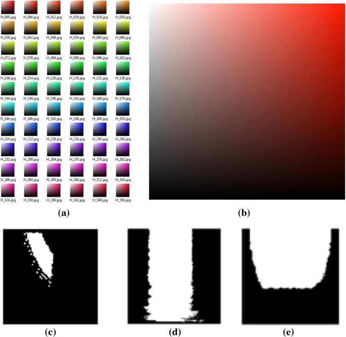

  

  Standard set of images used as a tool for evaluating different skin detection methods, proposed by Naji (2013); a The set of test images; b A test image used as input image to three methods shown in (c–e); c Skin detection results using Chen and Wang method (Chen and Wang 2007); d Skin detection results using Baskan’s method (Baskan et al. 2002); e Skin detection results using Solina’s method (Solina et al. 2002)

The performance of different skin detection methods is shown in Table 3.

Table 3 The performance of different skin detection methods

12 Conclusion

This study is an attempt to provide an up-to-date survey of research on skin detection methods that are described in over 150 research articles. Skin detection aims to segment the input image into regions in order to locate any exposed part of the human body. An improved human skin segmentation approach with higher detection rate enhances the performance of many computer vision applications. This stage is very important as image segmentation is considered to be the first step in image analysis and so, the overall success or failure of the whole system depends mainly on this step. Although in the last two decades a substantial progress has been made, there are many directions for future work. Researchers have to be aware that a robust skin detector should be effective against variation in: illumination conditions, different ethnic groups, image montage and reproduction, makeup, aging, and complex background.

A significant number of research articles have discussed the problem of color space selection and provided comparative studies and justifications for the optimality choice for the skin modeling and detection. It was noticed, however, that the HSV color space is superior in image segmentation due to its intuitive manner of specifying color as described in Sect. 8.

When available, we have reported the general performance of these methods. That being said, the methods in question appeared to use different raw datasets (i.e., training samples) which are collected manually by the researchers. The size and quality of raw data have a direct effect on the skin color clustering model even when various researchers use the same method. In other words, if new raw data of skin samples is collected from another database, the skin color cluster may change dramatically. Skin detection methods thus far have been largely subjective, leaving the researchers to decide the effectiveness of these methods because of the lack of uniformity on how to measure the correctness of a given clustering model and how these methods are evaluated. In general, most researchers perform their tests and experiments using their own datasets. Using different methods for modeling skin color clusters yields different classification boundaries (or clustering model) even with the same raw data. It is important to evaluate the feasibility of classification boundaries prior to any further testing steps. So, it is imprudent to decide which methods have the best detection performances. However, we have discussed the main strengths and limitations of each method in relation to critical issues such as simplicity, ease of adjustment, computational cost, memory requirements, size of training data, distribution shape, generality, and detection rates.

The way of processing and the final goals in these methods vary because they are intended to be used in different environments. Some methods are designed for a specific purpose in their approach and thus are inappropriate to be adapted for other applications without considering some underlying assumptions. Others have one or more tunable parameters which must be adjusted by the user rather than learned automatically from the image itself.

Exclude the illumination channel cannot help achieving better discrimination of skin regions when applied on complex images. Finally, the performance of skin detector depends on choosing the suitable color space in relation to certain environment.

There are a number of directions for future work. The deep learning techniques could be used to improve skin detection results. This may also allow the system to be trained with a smaller number of skin/non-skin examples than is currently used. Preprocessing steps are essential to exclude the background in order to avoid False Positives (FNs). Moving ahead, building a parallel processing implementation on GPUs hardware scheme to gain a substantial speed.

References

Adipranata R, Ballangan CG, Ongkodjojo RP (2008) Fast method for multiple human face segmentation in color image. In: Second international conference on future generation communication and networking, vol 2. Hainan Island, China, pp 158–161
Agathos A, Pratikakis I, Perantonis S, Sapidis N, Azariadis P (2007) 3D mesh segmentation methodologies for cad applications. Comput Aided Des Appl 4:827–841
Aghbari ZA, Al-Haj R (2006) Hill-manipulation: an effective algorithm for color image segmentation. Image Vis Comput 24:894–903
Ahlberg J, Ström J, Li H (1999) Extraction and coding of face model parameters. M.Sc. Thesis, Department of Electrical Engineering, Linköpings University, Sweden
Albiol A, Torres L, Bouman CA, Delp E (2000) A simple and efficient face detection algorithm for video database applications. In: International conference on image processing, vol 2. IEEE, Vancouver, BC, Canada, pp 239-242
Al-Mohair HK, Saleh J, Saundi S (2013) Impact of color space on human skin color detection using an intelligent system. In: 1st WSEAS international conference on image processing and pattern recognition (IPPR’13). pp 178–187, ISBN: 978-960-474-350-6
Al-Mohair H, Mohamad-Saleh J, Suandi SA (2014) Color space selection for human skin detection using color-texture features and neural networks. In: International conference on computer and information sciences (ICCOINS)
Amine A, Ghouzali S, Rziza M (2006) Face detection in still color images using skin color information. In: Proceedings of international symposium on communications, control, and signal processing (ISCCSP). pp 696–706
Barbu T (2014) Pedestrian detection and tracking using temporal differencing and HOG features. Comput Electr Eng 40:1072–1079
Baskan S, Bulut MM, Atalay V (2002) Projection based method for segmentation of human face and its evaluation. Pattern Recognit Lett 23:1623–1629
Bergasa LM, Mazo M, Gardel A, Sotelo MA, Boquete L (2000) Unsupervised and adaptive gaussian skin-color model. Image Vis Comput 18:987–1003
Brancati N, De Pietro G, Frucci M, Gallo L (2017) Human skin detection through correlation rules between the YCb and YCr subspaces based on dynamic color clustering. Comput Vis Image Underst 155:33–42
Bretzner L, Laptev I, Lindeberg T (2002) Hand gesture recognition using multi-scale colour features, hierarchical models and particle filtering. In: 2002 Proceedings of fifth IEEE international conference on automatic face and gesture recognition. IEEE, pp 423–428
Brown D, Craw I, Lewthwaite J (2001) A som based approach to skin detection with application in real time systems. In: Proceedings of the british machine vision conference. Citeseer, pp 491–500
Burdick HE (1997) Digital imaging: theory and applications. McGraw-Hill Inc, New York
Caetano TS, Olabarriaga SD, Barone DAC (2002) Performance evaluation of single and multiple-gaussian models for skin color modeling. In: Symposium on computer graphics and image. IEEE, pp 275–282
Cai J, Goshtasby A (1999) Detecting human faces in color images. Image Vis Comput 18:63–75
Carlsson A, Eriksson A, Isik M (2008) Automatic detection of images containing nudity. Master Thesis In intelligent systems design
Casati JPB, Moraes DR, Rodrigues ELL (2013) SFA: a human skin image database based on FERET and AR facial images. In: IX workshop de Visao computational. Rio de Janeiro
Chai D, Ngan KN (1999) Face segmentation using skin-color map in videophone applications. IEEE Trans Circ Syst Video Technol 9:551–564
Chai D, Phung SL, Bouzerdoum A (2001) Skin color detection for face localization in human-machine communications. In: Sixth international symposium on signal processing and its applications. IEEE, pp 343–346
Chai D, Phung S, Bouzerdoum A (2003) A Bayesian skin/non-skin color classifier using non-parametric density estimation. In: Proceedings of the international symposium on circuits and systems, vol 2. pp Ii-464–Ii-467
Chaichulee S, Villarroel M, Jorge J, Arteta C, Green G, Mccormick K, Zisserman A, Tarassenko L (2017) Multi-task convolutional neural network for patient detection and skin segmentation in continuous non-contact vital sign monitoring. In: 12th IEEE international conference on automatic face and gesture recognition (FG 2017)
Chauhan A, Farooqui Z (2016) An inventive approach for face detection with skin segmentation and multi-scale color restoration technique using genetic algorithm. Int J Res Comput Appl Robot 4(1):1–8
Chaves-González JM, Vega-Rodríguez MA, Gómez-Pulido JA, Sánchez-Pérez JM (2010) Detecting skin in face recognition systems: a colour spaces study. Digit Signal Process 20:806–823
Chen WC, Wang MS (2007) Region-based and content adaptive skin detection in color images. Int J Pattern Recognit Artif Intell 21:831
Chen Q, Wu H, Yachida M (1995) Face detection by fuzzy pattern matching. In: Fifth international conference on computer vision. IEEE
Chen F-S, Fu C-M, Huang C-L (2003) Hand gesture recognition using a real-time tracking method and hidden Markov models. Image Vis Comput 21:745–758
Cheng HD, Jiang X, Sun Y, Wang J (2001) Color image segmentation: advances and prospects. Pattern Recognit 34:2259–2281
Chin T (2008) Fuzzy skin detection. Thesis, Master of Science, Universiti Teknologi Malaysia
Cho KM, Jang JH, Hong KS (2001) Adaptive skin-color filter. Pattern Recognit 34:1067–1073
Dai Y, Nakano Y (1996) Face-texture model based on SGLD and its application in face detection in a color scene. Pattern Recognit 29:1007–1017
De Siqueira FR, Schwartz WR, Pedrini H (2013) Adaptive detection of human skin in color images. In: IX workshop de Visão Computacional (WVC). Rio de Janeiro-RJ, Brazil, pp 1–6
Do HC, You JY, Chien SI (2007) Skin color detection through estimation and conversion of illuminant color under various illuminations. IEEE Trans Consum Electron 53:1103–1108
Duan L, Cui G, Gao W, Zhang H (2002) Adult image detection method base-on skin color model and support vector machine. In: The 5th Asian conference on computer vision. pp 797–800
Duda RO, Hart PE, Stork DG (2001) Pattern classification. Hoboken, Willey
Dumitrescu CM, Dumitrache I (2016) Human skin detection using neural networks and block processing techniques. Univ Politeh Buchar Sci Bull Ser C Electr Eng Comput Sci 78:87–102
Efford N (2000) Digital image processing: a practical introduction using Java. Addison-Wesley Longman Publishing Co., Inc., New York
Fernandez A, Ortega M, Cancela B, Penedo M (2012) Human body parts contextual and skin color region information for locating human body parts. J Comput Inf Technol 1(1):1–16
Fleuret F, Geman D (2001) Coarse-to-fine face detection. Int J Comput Vis 41:85–107
Frisch AS, Vrschaeb R, Olanoc A (2007) Fuzzy fusion for skin detection. Fuzzy Sets Syst 158:325–336
Fu KS, Mui J (1981) A survey on image segmentation. Pattern Recognit 13:3–16
Garcia C, Tziritas G (1999) Face detection using quantized skin color regions merging and wavelet packet analysis. IEEE Trans Multimed 1:264–277
Gasparini F, Schettini R (2006) Skin segmentation using multiple thresholding. In: Proceedings of international imaging VII. pp 128–135
Gejguš P, Šperka M (2003) Face tracking in color video sequences. In: Proceedings of The 19th spring conference on computer graphics. ACM, pp 245–249
Ghazali KHB, Ma J, Xiao R (2012) An innovative face detection based on YCgCR color space. Phys Proc 25:2116–2124
Gomez G, Sanchez M, Sucar LE (2002) On selecting colour components for skin detection. In: 16th international conference on pattern recognition, vol 2. pp 961–964
Gonzalez RC, Woods RE (2002) Digital image processing. Prentice Hall Press, Englewood Cliffs
Gonzalez RC, Woods RE, Eddins SL (2007) Digital image processing using MATLAB. Prentice Hall Press, Englewood Cliffs
Greenspan H, Goldberger J, Eshet I (2001) Mixture model for face-color modeling and segmentation. Pattern Recognit Lett 22:1525–1536
Gupta A, Chaudhary A (2016) Robust skin segmentation using color space switching. Pattern Recognit Image Anal 26:61
Guru D, Sharath Y, Manjunath S (2010) Texture features and KNN in classification of flower images. IJCA Spec Issue RTIPPR 1:21–29
Habili N, Lim CC, Moini A (2004) Segmentation of the face and hands in sign language video sequences using color and motion cues. IEEE Trans Circ Syst Video Technol 14:1086–1097
Hai-Bo L (2012) A kind of human face region detection and recognition method based on chrominance information characteristics. In: 2012 International conference on control engineering and communication technology (ICCECT). IEEE, pp 469–472
Hajraoui A, Sabri M (2014) Face detection algorithm based on skin detection, watershed method and gabor filters. Int J Comput Appl 94:33–39
Han J, Awad G, Sutherland A (2009) Automatic skin segmentation and tracking in sign language recognition. Comput Vis IET 3:24–35
Hsieh C-C, Liou D-H, Lai W-R (2012) Enhanced face-based adaptive skin color model. 淡江理工學刊 15:167–176
Hsu RL, Abdel-Mottaleb M, Jain AK (2002) Face detection in color images. IEEE Trans Pattern Anal Mach Intell 24:696–706
Hua L, Abderrahim E, Jaral F, Su R (2003) An improved image segmentation approach based on level set and mathematical morphology. In: Third international symposium on multispectral image processing and pattern recognition. pp 851–854
Huang L, Xia T, Zhang Y, Lin S (2011) Human skin detection in images By MSER analysis. In: 2011 18th IEEE international conference on image processing (ICIP). IEEE, pp 1257–1260
Jain AK (1989) Fundamentals of digital image processing. Prentice-Hall, Inc., Englewood Cliffs
Jalab HA, Omer HK (2015) Human computer interface using hand gesture recognition based on neural network. In: 2015 5th national symposium on information technology: towards new smart world (NSITNSW). IEEE, pp 1–6
Jebara T, Russell K, Pentland A (1998) Mixtures of eigenfeatures for real-time structure from texture. In: Sixth international conference on computer vision. IEEE, pp 128–135
Jiang Z, Yao M, Jiang W (2007) Skin detection using color, texture and space information. In: Fourth international conference on fuzzy systems and knowledge discovery, 2007. FSKD 2007. IEEE, pp 366–370
Jones MJ, Rehg JM (2002) Statistical color models with application to skin detection. Int J Comput Vis 46(1):81–96
Juang CF, Shiu SJ (2008) Using self-organizing fuzzy network with support vector learning for face detection in color images. Neurocomputing 71:3409–3420
Kaabneh K (2014) Reliable skin detection using hybrid neural network model. Int J Adv Res Comput Commun Eng 3:5802–5805
Kakumanu P, Makrogiannis S, Bourbakis N (2007) A survey of skin-color modeling and detection methods. Pattern Recognit 40:1106–1122
Kawulok M, Kawulok J, Nalepa J (2014a) Spatial-based skin detection using discriminative skin-presence features. Pattern Recognit Lett 41:3–13
Kawulok M, Kawulok J, Nalepa J, Smolka B (2014b) Self-adaptive algorithm for segmenting skin regions. EURASIP J Adv Signal Process 2014:170
Khan R, Hanbury A, Stöttinger J, Bais A (2012) Color based skin classification. Pattern Recognit Lett 33:157–163
Khan R, Hanbury A, Sablatnig R, Stöttinger J, Khan FA, Khan FA (2014a) Systematic skin segmentation: merging spatial and non-spatial data. Multimed Tools Appl 69:717–741
Khan R, Hanbury A, Stöttinger J, Khan FA, Khattak AU, Ali A (2014b) Multiple color space channel fusion for skin detection. Multimed Tools Appl 72:1709–1730
Kim M, Park J, Joo Y (2005) New fuzzy skin model for face detection. Adv Artif Intell 3809:557–566
Kim C, You BJ, Jeong MH, Kim H (2008) Color segmentation robust to brightness variations by using B-spline curve modeling. Pattern Recognit 41:22–37
Kim Y, Hwang I, Cho NI (2017) Convolutional neural networks and training strategies for skin detection. In: 2017 IEEE international conference on image processing (ICIP). IEEE, pp 3919–3923
Kovac J, Peer P, Solina F (2003) Human skin colour clustering for face detection. In: The IEEE region 8 Eurocon 2003 computer as a tool, vol 2. pp 144–148
Kumar C, Bindu A (2006) An efficient skin illumination compensation model for efficient face detection. In: 32nd annual conference on IEEE industrial electronics. pp 3444–3449
Lee JY, Yoo SI (2002) An elliptical boundary model for skin color detection. In: Proceedings of the international conference on imaging science, systems, and technology
Lee JS, Kuo YM, Chung PC, Chen EL (2007) Naked image detection based on adaptive and extensible skin color model. Pattern Recognit 40:2261–2270
Li B, Xue X, Fan J (2007) A robust incremental learning framework for accurate skin region segmentation in color images. Pattern Recognit 40:3621–3632
Liu Z, Yang J, Peng NS (2005) An efficient face segmentation algorithm based on binary partition tree. Signal Process Image Commun 20:295–314
Ma Z, Leijon A (2010) Human skin color detection in RGB space with bayesian estimation of beta mixture models. In: 18th European signal processing conference (EUSIPCO-2010), Aalborg, Denmark
Ma W-Y, Zhang H (1999) Content-based image indexing and retrieval. In: Handbook of Multimedia Computing. CRC Press, pp 227–254
Mahmoodi MR (2017) High performance novel skin segmentation algorithm for images with complex background. arXiv:1701.05588
Martinkauppi B (2002) Face colour under varying illumination-analysis and application. Oulu University Library, Finland. Ebook: http://Herkules.Oulu.Fi/Isbn9514267885/, ISBN: 951-42-6788-5
MATLAB (2010) Version 7.11.0.584 (R2010b)
Mckenna SJ, Gong S, Raja Y (1998) Modelling facial colour and identity with Gaussian mixtures. Pattern Recognit 31:1883–1892
Medeiros R, Scharcanski J, Wong A (2013) Multi-scale stochastic color texture models for skin region segmentation and gesture detection. In: 2013 IEEE international conference on multimedia and expo workshops (ICMEW). IEEE, pp 1–4
Menser B, Wien M (2000) Segmentation and tracking of facial regions iIn color image sequences. In: Visual communications and image processing 2000. Perth, Australia, p 731
Moallem P, Mousavi BS, Monadjemi SA (2011) A novel fuzzy rule base system for pose independent faces detection. Appl Soft Comput 11:1801–1810
Moradi B, Ezoji M (2015) Skin detection based on contextual information. In: 2015 2nd international conference on pattern recognition and image analysis (IPRIA). IEEE, pp 1–6
Nadian-Ghomsheh A (2016) Pixel-based skin detection based on statistical models. J Telecommun Electron Comput Eng JTEC 8:7–14
Naji SA (2013) Human face detection from colour images based on multi-skin models, rule-based geometrical knowledge, and artificial neural network. Ph.D. Thesis, University Of Malaya, Malaysia
Naji S, Zainuddin R, Jalab H (2012) Skin segmentation based on multi pixel color clustering models. Digit Signal Process 22(2012):933–940
Oliver N, Pentland AP, Berard F (2000) LAFTER: A real-time face and lips tracker with facial expression recognition. Pattern Recognit 33:1369–1382
Osman MZ, Maarof MA, Rohani MF (2016) Towards integrating statistical color features for human skin detection. World Acad Sci Eng Technol Int J Comput Electr Autom Control Inf Eng 10:317–321
Pai Y-T, Lee L-T, Ruan S-J, Chen Y-H, Mohanty S, Kougianos E (2010) Honeycomb model based skin colour detector for face detection. Int J Comput Appl Technol 39:93–100
Peer P, Solina F (1999) An automatic human face detection method. In: Proceedings of computer vision winter workshop. pp 122–130
Perez M, Avila S, Moreira D, Moraes D, Testoni V, Valle E, Goldenstein S, Rocha A (2017) Video pornography detection through deep learning techniques and motion information. Neurocomputing 230:279–293
Phung SL, Chai D, Bouzerdoum A (2001) A universal and robust human skin color model using neural networks. In: International joint conference on neural networks, IJCNN 2001. Washington, DC. IEEE, pp 2844–2849
Phung SL, Bouzerdoum A, Chai D (2003) Skin segmentation using color and edge information. In: Seventh international symposium on signal processing and its applications, 2003. IEEE, Paris, France, pp 525–528
Phung SL, Bouzerdoum A, Chai D (2005) Skin segmentation using color pixel classification: analysis and comparison. IEEE Trans Pattern Anal Mach Intell 27(1):148–154
Pujol FA, Pujol M, Jimeno-Morenilla A, Pujol MJ (2017) Face detection based on skin color segmentation using fuzzy entropy. Entropy 19:26
Rahman MA, Purnama IKE, Purnomo MH (2014) Simple method of human skin detection using HSV and YCbCr color spaces. In: 2014 IEEE international conference on intelligent autonomous agents, networks and systems (INAGENTSYS). IEEE, pp 58–61
Rautaray SS, Agrawal A (2015) Vision based hand gesture recognition for human computer interaction: a survey. Artif Intell Rev 43:1–54
Razmjooy N, Mousavi BS, Soleymani F (2013) A hybrid neural network imperialist competitive algorithm for skin color segmentation. Math Comput Model 57:848–856
Roheda S (2017) A multi-scale approach to skin pixel detection. Electron Imaging 2017:18–23
Roth PM, Winter M (2008) Survey of appearance-based methods for object recognition. In: Inst. for computer graphics and vision, Graz University of Technology, Austria, technical report ICGTR0108 (ICG-TR-01/08)
Rowley HA, Jing Y, Baluja S (2006) Large scale image-based adult-content filtering. In: International conference on computer vision theory and applications 2006 Setúbal, Portugal, Citeseer
Ruijsscher B (2006) FPGA based accelerator for real-time skin segmentation, vol 4. Msc. Thesis, Delft University of Technology, Mekelweg
Russ JC (2007) The image processing handbook. CRC Press, Boca Raton
Sandeep K, Rajagopalan A (2002) Human face detection in cluttered color images using skin color and edge information. In: Indian conference on computer vision, graphics and image processing, 2002 ICVGIP 2002, Ahmadabad, India
Santos A, Pedrini H (2015) Improvements on human skin segmentation in digital images. M.Sc. Dissertation, Institute of Computing, University of Campinas, Brazil
Santos A, Paiva J, Toledo C, Pedrini H (2016) Improved human skin segmentation using fuzzy fusion based on optimized thresholds by genetic algorithms. In: Hybrid soft computing for image segmentation. Springer
Schmugge SJ, Jayaram S, Shin MC, Tsap LV (2007) Objective evaluation of approaches of skin detection using ROC analysis. Comput Vis Image Underst 108:41–51
Sebe N, Cohen I, Huang TS, Gevers T (2004) Skin detection: a bayesian network approach. In: Proceedings of the 17th international conference on pattern recognition. IEEE, Cambridge, UK, pp 903–906
Seow MJ, Valaparla D, Asari VK (2003) Neural network based skin color model for face detection. In: Proceedings of the 32nd applied imagery pattern recognition workshop (AIPR’03), Washington, DC, USA. IEEE, pp 141–145
Sevimli H, Esen E, Ateş TK, Ozan EC, Tekin M, Loğoğlu KB, Sevinç AM, Saracoğlu A, Yazıcı A, Alatan AA (2010) Adult image content classification using global features and skin region detection. In: Proceedings of the 25th international symposium on computer and information sciences. London, UK, pp 253–258
Shaik KB, Ganesan P, Kalist V, Sathish B, Jenitha JMM (2015) Comparative study of skin color detection and segmentation in HSV and YCbCR color space. Proc Comput Sci 57:41–48
Shapiro LG, Stockman G (2001) Computer vision. Prentice Hall, Englewood Cliffs
Shih FY, Cheng S, Chuang CF, Wang PSP (2008) Extracting faces and facial features from color images. Int J Pattern Recognit Artif Intell 22:515–534
Shin MC, Chang KI, Tsap LV (2002) Does colorspace transformation make any difference on skin detection? In: Sixth IEEE workshop on applications of computer vision (WACV 2002). IEEE, Orlando, Flordia, USA, pp 275–279
Siddiqui KTA, Wasif A (2015) Skin detection of animation characters. arXiv:1503.06275
Sigal L, Sclaroff S, Athitsos V (2000) Estimation and prediction of evolving color distributions for skin segmentation under varying illumination. In: Proceedings IEEE conference on computer vision and pattern recognition 2000, vol 2. IEEE, Hilton Head, SC, USA. pp 152–159
Sigal L, Sclaroff S, Athitsos V (2004) Skin color-based video segmentation under time-varying illumination. IEEE Trans Pattern Anal Mach Intell 26:862–877
Sobottka K, Pitas I (1998) A novel method for automatic face segmentation, facial feature extraction and tracking. Signal Process Image Commun 12:263–281
Solina F, Peer P, Batagelj B, Juvan S (2002) 15 seconds of fame-an interactive, computer-vision based art installation. In: 7th international conference on control, automation, robotics and vision, ICARCV 2002. IEEE, Singapore, pp 198–204
Sonka M, Hlavac V, Boyle R (2008) Image processing, analysis, and machine vision. Thomson Corporation, Stamford
Soriano M, Martinkauppi B, Huovinen S, Laaksonen M (2003) Adaptive skin color modeling using the skin locus for selecting training pixels. Pattern Recognit 36:681–690
Srisuk S, Kurutach W, Limpitikeat K (2001) A novel approach for robust, fast and accurate face detection. Int J Uncertain Fuzziness Knowl Based Syst 9:769–779
Storring M (2004) Computer vision and human skin colour. Ph.D. Thesis, Aalborg University, Denmark
Storring M, Kocka T, Andersen HJ, And Granum E (2003) Tracking regions of human skin through illumination changes. Pattern Recognit Lett 24(11):1715–1723
Sun H-M (2010) Skin detection for single images using dynamic skin color modeling. Pattern Recognit 43:1413–1420
Tan W, Chan C, Yogarajah P, Condell J (2012) A fusion approach for efficient human skin detection. In: IEEE transactions on industrial informatics. pp 1–1
Tao L (2014) An FPGA-based parallel architecture for face detection using mixed color models. arXiv:1405.7032
Taqa AY, Hamid J (2010) Increasing the reliability of fuzzy inference system-based skin detector. Am J Appl Sci 7:1129–1138
Taqa AY, Jalab H (2010) Increasing the reliability of skin detectors. Sci Res Essays 5:2480–2490
Terrillon JC, Shirazi MN, Fukamachi H, Akamatsu S (2000) Comparative performance of different skin chrominance models and chrominance spaces for the automatic detection of human faces in color images. In: Fourth IEEE international conference on automatic face and gesture recognition, 2000. IEEE, Grenoble, France, pp 54–61
Thakur S, Paul S, Mondal A, Das S, Abraham A (2011) Face detection using skin tone segmentation. In: 2011 world congress on information and communication technologies (WICT). IEEE, pp 53–60
Tomaz F, Candeias T, Shahbazkia H (2004) Fast and accurate skin segmentation in color images. In: First Canadian conference on computer and robot vision. IEEE, London, UK, Ontario, Canada, pp 180–187
Tsekeridou S, Pitas I (1998) Facial feature extraction in frontal views using biometric analogies. In: European association for signal processing EUSIPCO-98. Island of Rhodes, Greece, pp 315–318
Unnikrishnan R, Pantofaru C, Hebert M (2007) Toward objective evaluation of image segmentation algorithms. IEEE Trans Pattern Anal Mach Intell 29:929–944
Vadakkepat P, Lim P, De Silva LC, Jing L, Ling LL (2008) Multimodal approach to human-face detection and tracking. IEEE Trans Ind Electron 55:1385–1393
Varma SL, Behera V (2017) Human skin detection using histogram processing and gaussian mixture model based on color spaces. In: 2017 international conference on intelligent sustainable systems (ICISS). IEEE, pp 116–120
Verma A, Raj SA, Midya A, Chakraborty J (2014) Face detection using skin color modeling and geometric feature. In: 2014 International conference on informatics, electronics and vision (ICIEV). IEEE, pp 1–6
Vezhnevets V, Sazonov V, Andreeva A (2003) A survey on pixel-based skin color detection techniques. Graphicon 3:85–92
Wang Y, Yuan B (2001) A novel approach for human face detection from color images under complex background. Pattern Recognit 34:1983–1992
Wei G, Sethi IK (2000) Omni-face detection for video/image content description. In: The ACM workshops on multimedia. ACM, Los Angeles, CA, USA, pp 185–189
Xiaohua L, Lam KM, Lansun S, Jiliu Z (2009) Face detection using simplified gabor features and hierarchical regions in a cascade of classifiers. Pattern Recognit Lett 30:717–728
Yang MH (2000) Hand gesture recognition and face detection in images. Ph.D. Thesis, University Of Illinois, Urbana, Illinois
Yang MH, Ahuja N (1998) Detecting human faces in color images. In: IEEE international conference on image processing (ICIP-98). IEEE, Chicago, Illinois, USA, pp 127–130
Yang HM, Kriegman DJ, Ahuja N (2002) Detecting faces in images: a survey. IEEE Trans On Pattern Anal Mach Intell 24:34–58
Yoo T-W, Oh I-S (1999) A fast algorithm for tracking human faces based on chromatic histograms. Pattern Recognit Lett 20:967–978
Yuetao D, Nana Y (2011) Research of face detection in color image based on skin color. Energy Proc 13:9395–9401
Yusuf AA, Mohamad FS, Sufyanu Z (2017) Human face detection using skin color segmentation and watershed algorithm. Am J Artif Intell 1:29–35
Zafarifar B, Van Den Kerkhof T, De With PH (2012) Texture-adaptive skin detection for TV and its real-time implementation on DSP and FPGA. IEEE Trans Consum Electron 58:161–169
Zainuddin R, Naji S, Al-Jaafar J (2010) Suppressing false negatives in skin segmentation. In: Kim T, Lee Y, Knag B, Slezak D (eds) Lecture notes in computer science LNCS, vol 6485. Springer, Berlin, pp 136–144
Zaqout I, Zainuddin R, Baba S (2004) Human face detection in color images. Adv Complex Syst 7:369–383
Zarit BD, Super BJ, Quek FKH (1999) Comparison of five color models in skin pixel classification. In: International workshop on recognition, analysis, and tracking of faces and gestures in real-time systems ICCV ‘99. IEEE, sfdssf, Corfu, Greece, pp 58–63
Zhu Q, Wu C-T, Cheng K-T, Wu Y-L (2004) An adaptive skin model and its application to objectionable image filtering. In: Proceedings of the 12th annual ACM international conference on multimedia. ACM, pp 56–63
Zuo H, Fan H, Blasch E, Ling H (2017) Combining convolutional and recurrent neural networks for human skin detection. IEEE Signal Process Lett 24:289–293
Acknowledgements
The authors would like to thank Prof. Dr. Roziati Zaiuddin for her role as one of Sinan Naji’s Ph.D. supervisor and to the anonymous reviewers whose comments helped improve and clarify this manuscript.
Author information
Authors and Affiliations
Corresponding author
Ethics declarations
Conflict of interest
The authors declare that there is no conflict of interests regarding the publication of this article.
Rights and permissions
About this article
Cite this article
Naji, S., Jalab, H.A. & Kareem, S.A. A survey on skin detection in colored images. Artif Intell Rev 52, 1041–1087 (2019). https://doi.org/10.1007/s10462-018-9664-9
Published:
Issue Date:
DOI: https://doi.org/10.1007/s10462-018-9664-9