
Abstract
Dam-breaches that cause outburst floods may induce downstream hazards. Because landslide dams can breach soon after they are formed, it is critical to assess the stability quickly to enable prompt action. However, dam geometry, an essential component of hazard evaluation, is not available in most cases. Our research proposes a procedure that utilizes post-landslide orthorectified remote sensing images and the pre-landslide Digital Terrain Model in the Geographic Information System to estimate the geometry of a particular dam. The procedure includes the following three modules: (1) the selection of the reference points on the dam and lake boundaries, (2) the interpolation of the dam-crest elevation, and (3) the estimation of dam-geometry parameters (i.e., the height, length, and width), the catchment area, the volumes of barrier lake and landslides dam. This procedure is demonstrated through a case study of the Namasha Landslide Dam in Taiwan. It was shown the dam-surface elevation estimated from the proposed procedure can approximate the elevation derived from profile leveling after the formation of the landslide dam. Thus, it is feasible to assess the critical parameters required for the landslide dam hazard assessment rapidly once the ortho-photo data are available. The proposed procedure is useful for quick and efficient decision making regarding hazard mitigation.
Introduction
Landslides may block the river system and result in landslide dams. After the formation of a landslide dam, the natural lake always breached soon with an outburst flood that could induce disaster downstream. Based on a data set of 204 cases of dam failures, Peng and Zhang (2012) documented that half of the landslide dams failed within 1 week. Fan et al. (2012a, b) documented that 24 and 60 % of the landslide dams triggered by 2008 Wenchuan earthquake failed within 6 and 23 days, respectively. Catastrophic disasters caused by outburst floods and debris flows frequently occur soon after the formation of a barrier lake. It is, therefore, essential to assess the dam-breach hazards as rapid as possible (Schuster and Costa 1986).
The hazard due to the breach of a landslide dam can be expressed as the product of the probability of an outburst flood from the dammed lake (P(O/B)) and the probability of the downstream impact by an outburst flood (P(D/O)) (Korup 2005). The conditional probability P(O|B) is essentially a function of dam stability, whereas P(D/O) is the conditional probability of spatial impact by a landslide dam-break flood, given the failure of a landslide dam. Dam stability can be evaluated by using geotechnical and hydrogeological analyses. Physically based hydraulic models for breach analysis and the downstream propagation of outburst floods are able to predict the breach-outflow hydrograph, flood parameters (e.g., flood depth and velocity), and inundation area downstream of a landslide dam (e.g., Li et al. 2011). To build the numerical model and to collect the required input parameters, however, are both time consuming. In addition, the results of the analyses are sensitive to input properties of the dam materials, such as grain-size characteristics and the shear strength of the debris (Evans et al. 2011).
Empirically, the risk for landslide dams induced by the 2008 Wenchuan earthquake in China was classified, according to landslide dam height, lake capacity, and dam materials, into the following four risk levels: (1) extremely high, (2) high, (3) medium, and (4) low (Yin et al. 2009; Xu et al. 2009; Cui et al. 2009). This empirical approach is easy to use and is effective for decision making under emergency. However, the roles of the landslide dam failure and the impact (consequence) of the outburst flood from the dammed lake are not evaluated separately. It is possible to evaluate the related hazard by combining the estimations of the failure probability of a landslide dam and the impact of the outburst flood from a breached landslide dam (Dong et al. 2011a; Yang et al. 2012).
Currently, the geomorphic approach is widely used to correlate the landslide dam stability with the characteristics of the dam, river flow, and lake volume (Costa and Schuster 1988; Ermini and Casagli 2003; Korup 2004; Dong et al. 2009, 2011a) and to estimate the peak outflow discharge following a breach of the landslide dam (Costa 1985; Costa and Schuster 1988; Walder and O’Connor 1997; Peng and Zhang 2012). For example, the failure probability of a landslide dam can be calculated by a logistic regression model using the dam geometry parameters (e.g., the upper catchment area, the dam height, width, and length) (Dong et al. 2011a). Among the relevant factors, the peak discharge of the dam-breach flood is the most important factor dominating the impact of the dam-breach flood (Korup 2005). The peak discharge of a dam-breach flood can be estimated empirically or calculated numerically. Xu and Zhang (2009) pointed out the empirical formulae based on case studies are more preferable when a database of numerous well-documented dam failure cases is available. Peng and Zhang (2012) compiled and compared several empirical formulas for predicting the peak flood discharge based on a comprehensive dataset of landslide dams. Among others, lake volume and dam height have been used as effective indicators of peak discharge.
The aforementioned geometric characteristics of a landslide dam are critical factors relevant to hazard evaluation; they include upstream catchment area (A), dam height (H), dam length (L), dam width (W), dam volume (V d ), and lake volume (V l ). However, in most cases, it is very difficult to obtain these geomorphic characteristics within the first week after the formation of a landslide dam. Yet, 1 week may be too long because half of the historical cases failed within 1 week (Peng and Zhang 2012). Therefore, it is a critical issue in risk management and hazard mitigation to enable the rapid characterization and measurement of the geomorphometric parameters of the dam and the lake, even just for approximation.
In situations where the pre- and post-landslide digital terrain models (DTM) are available, dam geometry can be obtained from a Geographic Information System (GIS) platform, without much difficulty. However, only the pre-landslide topography is readily available for the rapid hazard assessment of a landslide dam, in most cases. High-resolution airborne LiDAR (Light Detection and Ranging) has been utilized successfully to evaluate the geomorphological characteristics of large landslides and their induced landslide dams (e.g., Chang et al. 2006; Chen et al. 2006). However, the production of a DTM from LiDAR is time consuming and is often impossible to complete in time to assess the hazards of a landslide dam-breach effectively. Dong et al. (2011b) utilized post-landslide ortho-images and pre- and post-landslide DTMs to evaluate the geometry of the partially breached Hsiaolin landslide dam. By integrating a hydrology analysis, laboratory work, and extensive field investigation results, they successfully reconstructed the dam’s geometry. However, field investigations at the sites of newly formed landslide dams are very often difficult and dangerous. The needs of such investigations raise the following three questions. First, is it possible to derive the geometry of the dam with an acceptable accuracy using only post-landslide remote sensing images and pre-landslide DTM? Second, to what extent will the resolution of remote sensing images and DTM affect the results of the dam-geometry evaluation? Finally, how much time is required to evaluate the hazards of a landslide dam to perform first-order estimation? This work aims to answer these questions and to propose a feasible procedure utilizing post-landslide orthorectified remote sensing images, pre-landslide DTM in order to extract the geometry of a landslide dam. To test the proposed procedure, a landslide dam case occurred in Taiwan is studied; the present work compares the estimated dam profiles with the actual cross-sections obtained by profile leveling after the formation of the landslide dam. Subsequently, the implications of the proposed procedure for rapid assessment of the hazards due to dam-breach floods are discussed. The influence of the resolutions of remote-sensing images and DTM data on the estimated dam geometry is also examined. Finally, the related uncertainty of the proposed procedure is assessed.
Procedure for evaluating the landslide dam geometry
A feasible procedure for the rapid estimation of dam geometry is developed in this research. Figure 1 illustrates the proposed procedure using the post-landslide orthorectified remote-sensing image and the pre-landslide DTM. The proposed procedure contains the following three main modules: (a) selecting the reference points (items 7–10); (b) interpolating the elevation of the dam crest (item 11); and (c) estimating the dam geometry, the dam volume, the lake storage volume, and the catchment area (items 14–15).

Proposed procedure for the evaluation of dam geometry, dam volume, lake volume, and catchment area
Selecting the reference points on the dam and lake boundaries
If a clear remote-sensing image is available, the image can be used to identify the location of a newly formed landslide dam and barrier lake. After interpreting the landslide, dam, and lake as polygons (Item 6), the elevation of points with proper interval along the boundaries of the dam- and lake-polygons could be determined sequentially based on the pre-landslide DTM (item 7). The interval of the selected boundary points should not be smaller than the resolution of the DTM. Three types of reference points can be identified from the points located on: (a) barrier lake boundary; (b) dam-lake boundary; (c) dam boundary (Fig. 2). The averaged elevation of the reference points along the barrier lake boundary (the triangles in Fig. 2) indicates the water level of the lake. Since the elevation of the dam crest along the dam-lake boundary should be identical to that water level, the elevations of the reference points along the dam-lake boundary (see the squares in Fig. 2) can be assigned with the value of determined water level (item 10). Other auxiliary approach can also be applied to derive the water level of the lake. Contours extracted from a pre-landslide DTM can be overlapped on the ortho-photo using a GIS platform. The elevation of the best-fitted contour to the barrier lake boundary indicates the water level of the lake; the water level of the lake may increase slightly to the upstream.

Illustration for the determination of the reference points on the dam and lake boundaries
The dam boundary is identifiable from the boundary of vegetated and bare land (see the circles in Fig. 2). Figure 2 illustrates the determination of the reference points on the dam surface. It is important to note that landslides and erosion on the riverbanks may seriously disturb the determination of the dam crest. Meanwhile, the dam boundary is vague in the shadow zones of the images. To minimize the errors for the determination of the reference points, it should be careful to exclude the points on the zones of landslides, erosion, and shadows on river banks (as illustrated in Fig. 2).
Interpolating the elevation of the dam surface
To determine the elevation of the landslide dam surface is the most important step for deriving the landslide geometry from a remote-sensing image. After the reference points of the dam surface (on the dam lake boundary and dam boundary) with assigned elevations are properly identified, the elevation of the dam surface can be interpolated using the interpolation function of GIS.
To estimate the upstream shape of the landslide dam that will eventually become submerged, it is better to obtain multi-temporal remote sensing images and to identify temporal reference points from the rising water level of the barrier lake. The most difficult challenge is to evaluate the elevations of the submerged dam surface when the multi-temporal remote sensing images are not available. One method for estimating the elevation of a submerged dam surface is to assume that shape of the submerged part of the dam is similar to its adjacent un-submerged part. Consequently, the elevation of the submerged dam can be extrapolated with the assumed slope of the dam surface. Alternatively, Kuo et al. (2011) proposed an empirical relationship that correlates the river slope and the dam slopes in both the downstream and the upstream directions. That type of empirical relation can also be adopted to estimate the upstream submerged dam shape. For the determination of the dam boundary in the downstream, the downstream reference points should be used to interpolate the dam shape. Generally, a slope-break point, where the steep downstream dam slope turns into a gentle slope close to the channel gradient, indicates the dam boundary in the downstream.
Determining the dam geometry, dam volume, lake storage volume, and catchment area
From the interpolated dam-crest elevation and the boundaries of the landslide dam and barrier lake, the required variables for hazard assessment, including height (H), transverse (cross-river) length (L), longitudinal (along-river) width (W) of the dam, the volume of the dam (V d ), and the lake storage volume (V l ), can be evaluated by following the steps together with a proper GIS platform (e.g., the ArcHYDRO).
-
Step 1
The height (H) and transverse length (L): H and L are measured from a cross-section (perpendicular to the river channel) passing through the overtopping point (Fig. 3a).
Fig. 3 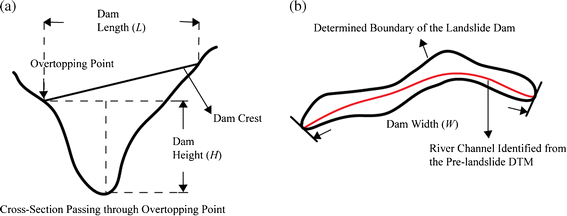
Definitions of the height, length, and width of a landslide dam
-
Step 2
The longitudinal width (W): W is measured from the identified boundary of the landslide dam along the river channel identified from the pre-landslide DTM (Fig. 3b).
-
Step 3
The volume of the dam (V d ): V d is calculated from the elevation differences of the pre-landslide DTM and the evaluated post-landslide DTM (deposition thicknesses).
-
Step 4
The volume of the lake storage (V l ): V l is calculated from the lake depths determined from the lake polygon, water level, pre-landslide DTM, and the evaluated post-landslide DTM (submerged part of the landslide dam). V l can be related to the water level of the dammed lake. The maximum volume of lake storage should be determined.
-
Step 5
The catchment area (A): A can be calculated from the pre-landslide DTM.

The determination of the dam height (H), cross-river dam length (L), and the upstream catchment area (A) is related to the overtopping point on the crest of the landslide dam. If satellite image was taken after the dam was overtopped, the location of the overtopping point could be identified easily from the image. However, if the satellite image was acquired before overtopping, it is practically difficult to determine the overtopping point from the image directly. In that situation, the contours of the landslide dam crest can be generated first (Fig. 1), then the overtopping point can be estimated preliminarily. The first step is to determine the highest point of the dam crest along the river. Secondly, draw a cross-section through the highest point perpendicular to flow direction. Finally, the lowest point of the cross-section can be regarded as the overtopping point. If possible, multi-temporal images may help to update the interpolated dam surface till the dam is overtopped (Fig. 2).
Temporal variation of the water level of a barrier lake is useful to estimate the inflow discharge from the upstream area; it can be determined from the multi-temporal remote-sensing images with identified elevations of the reference points on the barrier lake boundary (items 17–18). The water level of the barrier lake is one of the crucial data for determining lake volume. The variation in lake volume can be determined if multi-temporal remote-sensing images are available. Notably, if the landslide dam were already overtopped, the elevation of the dam crest at the overtopping (or breaching) point should be identical to the determined water level.
Validation of the proposed method for dam geometry evaluation
Namasha landslide dam
In 2009, Typhoon Morakot brought intense rainfall to southern Taiwan. The total rainfall 2,138 mm accumulated from Aug. 7 to 11 was recorded from the Jiashian 2 raingauge stations (Fig. 4). The peak hourly rainfall intensity was 95 mm/h, and the rainfall duration was 99 h. The heavy rainfall triggered 17 large landslides that resulted in the formation of landslides dams (Chen and Hsu 2009). Namasha Landslide Dam is one of them, located at Minshan Village, Southern Taiwan (Fig. 4; X: 120°44′39.44″ and Y: 23°19′39.49″). The source area of the Namasha landslide is approximately 0.6 km2. The debris that flowed down the creek and the resulting deposition fan dammed the Cishan River. Figure 5 shows the geologic map with a scale of 1:50,000 (Sung et al. 2000). Miocene Changchikeng Formation (Cc) outcrops are visible at the landslide site. Figure 6 shows the post-landslide ortho-image taken by the Aerial Survey Office, Forestry Bureau of Taiwan (ASOFB) near the Namasha Landslide Dam. The Namasha Landslide Dam and the barrier lake can be clearly identified in Fig. 6. Since overtopping occurred soon after its formation, multi-temporal images with different water level are unavailable.

The location of the Namasha Landslide and the landslide dam at Minshan Village, Southern Taiwan. The rectangular frame represents the area shown in Fig. 5

The 1:50,000-scale geologic map near the Namasha Landslide Dam site. The landslide source area is approximately 0.6 km2. The Miocene Changchikeng Formation (Cc) outcrops at the landslide site. The rectangular frame represents the area that is shown in Fig. 6

This aerophoto was taken on Aug. 24, 2009, approximately 2 weeks after the Typhoon Morakot, by the Aerial Survey Office, Forestry Bureau of Taiwan (ASOFB). The barrier lake boundary (yellow long dashed line), dam-lake boundary (pink solid line), and dam boundary (blue short dashed line) are marked. The rectangular frame represents the area that is shown in Figs. 7 and 10
Dam Geometry Evaluation for the Namasha Landslide Dam
The proposed method is applied in this subsection to determine the geometry of the Namasha Landslide Dam, then verified with the measured cross-sections in the following subsection. The post-landslide ortho-aerophoto (with a resolution less than 0.5 m) and the pre-landslide DTM (approximately 5 m per pixel) provided by ASOFB were used to evaluate the dam geometry.
The post-landslide image used was taken on Aug. 24, 2009, about 2 weeks after the dam formation. At that time, overtopping had already occurred; the overtopping point at E: 224034 and N: 2579895 (TWD97) can easily be identified in Fig. 6. The catchment area of the landslide dam (A) was determined to be 213 km2.
The boundaries of the dam- and lake-polygons are determined based on the post-landslide ortho-image. The selected boundary points are in 5-m interval which is compatible with the resolution of the 5-m DTM. Three types of reference points are selected from the boundary points on: (a) the barrier lake boundary; (b) the dam-lake boundary; and (3) the dam boundary (Fig. 6). These selected reference points are away from the influence areas of the landslide and erosion on the riverbanks, as well as the shadow zone. The elevation of the barrier lake boundary is determined first. Because the view direction of this image is toward the northwest, the vegetation obscures the observation of the barrier lake boundary on the southeastern bank of the barrier lake. Along the northwestern bank, the averaged elevation of the selected reference points (200 points) on the barrier lake boundary is 795.3 m with a standard deviation of 4.9 m. This averaged elevation of the reference points indicates the water level of the barrier lake. For the Namasha Landslide Dam already with overtopping, the dam-crest elevation at the overtopping point is identical to the determined water level. The averaged water level from the selected reference points (391 points) on the southeastern bank is 784.1 m. It appears that the water level will be underestimated if the reference points for the lake boundary on the southeastern bank are used; the standard deviation of the estimated elevation for the southeastern lake boundary is 10.9 m, which is roughly twice larger than that derived from the reference points on the northeastern bank. The effect of the view direction of the image will be discussed later. As discussed in ““Procedure for evaluating the landslide dam geometry” section, the elevation of the best-fitted contour to the lake boundary also indicates the water level of the lake. The best-fitted elevation of the water level is approximately 795 m, which is close to the determined water level from the reference points on the barrier lake boundary.
From the water-level elevation of the lake, the elevations of the reference points along the dam-lake boundary can be determined as 795.3 m (represented by red squares in Fig. 7). The reference points on the boundary of vegetated and bare land are also marked in Fig. 7 (blue circles). The linear interpolation function of ArcGIS is used to interpolate the dam surface contours. Figure 7 shows the result of interpolation using the reference points on the dam-lake boundary and the dam boundary. The contours of the upstream dam display the topography in a fan shape. This is understandable since the Namasha Landslide Dam is formed at the tip of a debris flow fan. The inclination angle of the deposition fan is about 6.4°. Based on field investigations in Taiwan, Shieh and Tsai (1997) reported that the slope of the deposition fan arisen from debris flow is generally within 6–10°.

The reference points and the interpolated contours of the dam surface. The purple lines represent the contours of the estimated dam surface
Because part of the upstream dam is submerged, we assume that the inclination angle of the submerged dam is also 6.4°. At this juncture, the elevation of the submerged dam can be extrapolated. Contours are created as concentric circles with a slope of 6.4°. The boundary of the submerged dam is determined accordingly; the elevations of the circles are identical to those of the contours interpolated from the pre-landslide 5-m DTM. The elevations of the dam surface are re-interpolated with those newly added reference points of submerged dam, again using GIS.
The channel bed of the Cishan River elevated more than 20 m after 2009 Typhoon Morakot; therefore, the downstream dam boundary is difficult to be determined precisely. A longitudinal profile is obtained from the interpolated dam surface. The slope-break point with the elevation of 747 m on the downstream interpolated dam surface can be identified where the steep slope of the downstream dam surface abruptly changed to a gentle one. Accordingly, the interpolated contour of 747 m is assumed as the downstream dam boundary. The contours of the whole dam surface can be produced (the purple lines in Fig. 7); consequently, the geomorphic parameters of the dam can be evaluated.
Verification of the proposed method
Following the formation of the Namasha Landslide Dam, the Forestry Bureau of Taiwan selected seven transverse profiles (A1–A7 in Fig. 7) to monitor elevation changes (Taiwan Forestry Bureau 2010). To verify the proposed method for the determination of dam geometry, the cross-sections measured approximately 2 months after the dam formation (Oct. 29, 2009) were compared with the results derived from the post-landslide remote sensing images and pre-landslide DTM. Figure 8 compares the measured cross-sections with those obtained from the proposed procedure. The differences are generally within 10 m; the dam shape evaluated by the proposed approach is consistent with the field measured results. The slightly lower elevation of the evaluated dam surface along the southeastern bank was likely owing to the viewing direction of the photo taken. The underestimation in the elevation of dam surface related to the images will be discussed later. Figure 9 shows the longitudinal profile of the Namasha Landslide Dam (vertical exaggeration by 2). The dam profile was obtained based on the contours produced using the proposed procedure. The evaluated profile is slightly lower than the field measured results as discussed above. Notably, the river bed downstream the dam was elevated about 30 m; we speculated that the river bed upstream the dam could also be elevated (the dash line in the upstream of the dam).

The evaluated dam crests and the measured cross-sections of the seven profiles of the Namasha Landslide Dam.

The longitude profile of the Namasha Landslide Dam with the dam crest determined by the proposed procedure
Based on the evaluated elevation of the dam crest, the dam height (H) was 55 m and the deepest deposit was about 60 m thick. The transverse length (L) passing through the overtopping point was 225 m. The longitudinal width (W) of the dam was 1,935 m. The volume of the landslide dam (V d ) can be calculated using the pre-landslide and interpolated post-landslide DEMs (sum of the elevation difference of each pixel of the dam multiple by the pixel area). Figure 10 shows the elevation difference (deposition thickness) between the pre-landslide and post-landslide DTM. The calculated volume of the landslide dam was approximately 8.7 × 10⁶ m3. The lake volume (V l , sum of the water depth of each pixel of the lake polygon multiple by the pixel area) was approximately 9.7 × 10⁶ m3 (the influence of sediments from the upstream region following Typhoon Morakot was not taken into account). Notably, the minus deposition depth (cold colors) can be observed near the erosion bank. These parts are excluded when calculating the dam volume. Accordingly, the dam volume will be underestimated.

The elevation difference (deposition thickness) between the pre-landslide and post-landslide DTM. The red line indicates the cross-section used to calculate the dam height and dam length
Discussion
Rapid assessment of the critical parameters related to landslide dam hazards
To evaluate the hazard related to the dam-breach flood, the failure probability of the dam and the impact of the breach flood are crucial as aforementioned. Dong et al. (2011a) proposed a logistic regression model to calculate the failure probability of landslide dams as follows:
where A(in meter squared), H (in meter), W (in meter), and L(in meter) are the catchment area upstream of the landslide dam and the dam height, dam width, and dam length, respectively. The logit, represented by L s , is the measure of the total contribution of all the variables (A, H, W, and L). The failure probability of a landslide dam can be calculated from L s using \( {{{{P_f}={e^{{-{L_S}}}}}} \left/ {{\left( {1+{e^{{-{L_S}}}}} \right)}} \right.} \). The condition L s = 0 corresponds to the condition that the probability of a landslide dam failure is 50 %. Dams with variables such that L s > 0 are classified as stable, and all other dams are classified as unstable. Using Eq. (1), the failure probability of the Namasha Landslide Dam was 88 % because the evaluated catchment area of the landslide dam (A) was 213 km2, dam height (H) was 55 m, the longitudinal width (W) of the dam was 1,935 m, and the transverse length (L) was 225 m.
The spatial impact of the dam-breach flood is related to peak discharge and downstream topography. The equation proposed by Costa (1985),
is utilized for illustration, where V i (in 106 m3) is the lake (storage) volume and H (in meter) is the dam height. As discussed above, the Namasha Landslide Dam impounded 9.7 × 10⁶ m3 water with a height of 55 m. Using Eq. (2), the estimated peak discharge is 2,690 m3/s. According to the management plan of the Water Resources Agency of Taiwan, the watershed in the upstream of the Yuemei Bridge (indicated in Fig. 4) on the Cishan River is approximately 533 km2 and the allowable discharge is 5,680 m3/s. The ratio of the peak discharge (specific discharge) at two cross-sections of a stream Q u /Q d (Q u and Q d denote the peak discharges at a upstream and a downstream cross-sections, respectively) can be estimated by \( {{{({A_u}}} \left/ {{{A_d}}} \right.}{)^n} \), where \( {A_u} \) and \( {A_d} \) are the catchment areas at the upstream and downstream cross-sections, respectively (Creager et al. 1950). With n = 0.98, calibrated through the peak discharges during two typhoon events near the study area, the allowable discharge of the stream section near Namasha is estimated to be 2,310 m3/s. Hence, the estimated peak discharge of the dam-breach flood exceeds the allowable discharge by 16 %.
It took less than eight man-hours (i.e., one researcher took 8 h) to derive the elevation of the dam crest and to obtain the relevant parameters for the downstream hazard for the Namasha case. Chen et al. (2005) reported that for a test site with an area of 3,600 km2, an ortho-photo from a SPOT5 image can be produced in 28 min by adopting an “adaptive patch projection” scheme. Accordingly, the critical parameters related to the dam-breach hazard may be assessed promptly after a clear aerial image is available. The demonstration reveals that the proposed procedure may be useful and feasible for a first-phase evaluation of the hazard related to the potential outburst from a landslide dam-breach.
Notable, Eqs (1) and (2) are derived from limited case histories. These prediction models can be substituted if other suitable models are available. Since the factors dominating the stability and breaching process of a landslide dam are highly related to the geomorphological, geological, and hydrogeological environment, proper and careful selection of the prediction models is strongly recommended.
Influence of the image and DTM resolution
An aerophoto is not always readily available after the formation of a landslide dam. FORMOSAT-2 has a relatively high spatial resolution (2-m panchromatic) and a high temporal resolution (1 day). This study used an ortho-photo from a FORMOSAT-2 satellite image acquired on Aug. 15, 2009 and a 40-m DTM to evaluate the influence of data resolution on the hazard evaluation results.
We first evaluate the influence of image and DTM resolutions and precisions on the determined water level of the barrier lake from the reference points of the lake boundary. Notably, the reference points on the barrier lake boundary are selected at an interval compatible to the resolutions of DTMs; 40-m interval of reference points are selected if a 40-m DTM is used. The 40-m resolution DTM is digitized from the 1/5,000–1/10,000 topography map with 5- to 10-m contours. Theoretically, the vertical precision is 2.5 to 5 m for the 40-m resolution DTM whereas the related errors are difficult to be evaluated. The vertical precision of the 5-m resolution DTM depends on the steepness of the topography and thickness of the vegetation. It should be noted the height of forest affects the precision. For a mountain area covered by dense forest with 10 m in height, the vertical precision of the used 5-m DTM is 2.9 m.
Table 1 shows the mean values and standard deviations of the reference points on the northwestern side of the barrier lake boundary derived from image and DTM with different resolution. From Table 1, it can be observed that the variation of the inferred water level (the mean elevation of the reference points on the barrier lake) determined from image and DTM with different resolution is within 10 m (the inferred water level ranges from 788.3 to 798.3 m). As expected, the elevation for reference points derived from the aerophoto and 5-m DTM has the lowest standard deviation (4.9 m). The elevations of the reference points derived from the FORMOSAT-2 image and 40-m DTM has the highest standard deviation (12.4 m). Without surprise, the standard deviation increases with decreasing resolutions of images and DTMs. The resolutions of the used images (shown in Table 1) are less than those of the used DTMs. It seems that the variation of the inferred water level is compatible to the resolution and vertical precision of the DTMs.
Using the post-landslide FORMOSAT-2 satellite image and pre-landslide 40-m DTM, the evaluated dam height, dam length, and dam width were 47, 240, and 2,000 m, respectively. Hence, the failure probability of the dam was 83 %, and the peak discharge of the outburst flow was 2,400 m3/s. Compared with the results generated using the ortho-aerophoto image and the 5-m DTM (i.e., failure probability = 88 % and peak discharge = 2,690 m3/s), the difference in the dam failure probability is approximately 6 %, and the difference in outburst flow is approximately 11 %. It can be found that there are insignificant differences on the dam width and length values determined from data with different resolution (Table 2) since the resolution of the FORMOSAT-2 image is high. DTM resolution only affects the dam height (H). It appears that the resolutions of the FORMOSAT-2 satellite image and the 40-m DTM are acceptable for the first-phase evaluation of a landslide dam-breach hazard. We also tried to use an image with 20-m resolution (SPOT 4) to identify the reference points. However, the resolution is not high enough to distinguish the lake and dam boundaries. It is suggested to use satellite image with its resolution less than 20 m for the application of the proposed procedure.
Uncertainty for the determination of the dam geometry from image and DTM
As illustrated in Fig. 11a, the view direction of the remote-sensing image will induce error for identifying the elevation of a reference point. This error cannot be eliminated with an orthorectified image. For the Namasha Landslide case, the determined water level from the reference points on the southeastern bank (on the slope with dip direction against to the view direction of the image) is 5 m less than that determined from the reference points on the northwestern bank. Also, it is notable the standard deviation of the elevations of the reference points on the southeastern bank (on the slope with dip direction against to the view direction of the image) is larger than that calculated from the reference points on the northwestern bank.

The error induced by a the view direction of images and b the shadow zone
Three factors dominate the induced error from the view direction of the remote sensing image. First, vegetation obscures the observation of the barrier lake boundary and dam boundary. Generally, the error of the estimation can be related to the width and height of the tree (Wt and Ht in the Fig. 11a). Second, this error tends to increase with increasing slope angle. Finally, the error of the estimated elevations of the reference points on the slope with dip direction against the view direction (error A) is smaller than that on the slope with dip direction along the view direction (error B).
For the Namasha case, the measured elevations of the dam crest are generally higher than the evaluated ones (Fig. 8). The cross-sections were measured by profile leveling 2 months after the dam formation; the evaluated ones were obtained using the images taken 2 weeks after the damming event. It is possible that the elevation differences in the profiles may be attributed to the erosion and sediment transport. As aforementioned, the water level determined from the lake boundary of the northwestern bank was 795.3 m whereas that determined from the southeastern side was 784.1 m. It appears that the elevations of the dam boundary determined from the reference points on the southeastern side of the dam could be underestimated. The related error was roughly estimated to be about 10 m in the Namasha case. Interestingly, the evaluated cross-sections are systematical lower than the measured results. If we added the error calibrated from the barrier lake boundary to the reference points on the southeastern side of the dam, the evaluated cross-sections will match the measured results perfectly (e.g., A2–A4 in Fig. 8). Development of a technology for correcting the error induced from the view direction of the image is in need.
The other uncertainty comes from the shadow zone (Fig. 11b). This research eliminated the points on the boundaries where large shadow zone existed. Therefore, the interpolation uncertainty would be higher near those shadow zones. Since the images of the Namasha case is taken in the morning, the shadow zone is mainly distributed on the northwestern slope. The effect also accounts for the large standard deviation in the elevations of the reference points on the barrier lake boundary along the northwestern bank. The interpolation uncertainty would be higher near the river bank where the erosion and landslides occurred. Errors could also be induced from the orthorectify and geocode process. Generally speaking, the error encountered in the orthorectified and geocoded image is less than tens of centimeter, which is minor comparing with the aforementioned uncertainty.
The extrapolation of the elevation of dam crest across the river may induce error since the dam shape is always irregular. Dam crest elevations are well constrained on the dam boundary. However, it is difficult to evaluate the dam crest elevations away from the riverbank only based on a post-landslide image and pre-landslide DTM. Interpolation of the reference points yields a smooth variation of the dam-surface elevations. The interpolation will yield a good result if the elevation of the dam surface varies linearly (Fig. 12a). For a curved dam surface (e.g., Fig. 12b), error in interpolation can be expected. The Hsiaolin landslide dam in Taiwan (Dong et al. 2011b) and the Tangjiashan landslide dam in China (Xu et al. 2009) were two examples of large, quick-moving landslides which formed a concaved upward dam surface. In fact, the shape of a landslide dam, in general, is far from the idealized one; the uncertainty nduced from the interpolation scheme is difficult to be evaluated. The landslide type, the transportation and deposition processes, and the morphology of the valley, all affect the shape of the landslide dam. This subject may deserve further study and will be helpful for the characterization of landslide dam morphology.

Schematic figure showing the dam shapes with a linear variation and b non-linear variation
Limitations of the proposed method
Landslide dams induced by heavy rainfall are frequently short-lived. For example, the Hsiaolin landslide dam in southern Taiwan failed within 1 h after its formation (Dong et al. 2011b). Unfortunately, clear images are not rapidly available after the occurrence of a landslide because the remote-sensing image may be blocked by clouds during and after a rainfall event. From the hazard-mitigation perspective, little can be achieved in the case of such rapidly breaching landslide dams. In general, an earthquake-induced landslide dam can usually be identified more rapidly than a rainfall-induced landslide dam. In addition, the elapsed time to overtop an earthquake-induced landslide dam is usually much longer than that for a rainfall-induced dam. Consequently, the former allows a longer time for the estimation of their geomorphic characteristics before overtopping. Small dams often breach soon before the mobilization of site investigation; larger dams usually can survive relatively longer. The proposed method to evaluate landslide dam geometry is more suitable for a landslide dam not promptly breached after its formation.
Conclusions
This research proposed a procedure that utilizes post-landslide remote sensing images and pre-landslide DTM to rapidly and accurately evaluate dam geometry. Based on the Namasha case, the error in the estimated elevation of the dam crest is generally less than 10 m when compared with the data from profile leveling. We demonstrated that the critical parameters relating to the hazards from a dam-breach may be assessed rapidly after a clear ortho-photo is available from remote sensing. In our case study, the failure probability of the dam is 88 % and the peak discharge of the outburst flow is 2,690 m3/s. For comparison, using the satellite image and 40-m DTM, the evaluated failure probability of the dam becomes 83 %, and the peak discharge of the outburst flow becomes 2,400 m3/s. For the two resolution combinations of images and DTM, the difference in the evaluated susceptibility of dam failure is 6 %, and the difference in the outburst flow is 11 %. This case demonstrates that the geomorphic characterization of a landslide dam using post-landslide images and pre-landslide DTM can be efficiently applied for the emergent assessment of the hazard associated with a landslide dam.
References
Chang KJ, Taboada A, Chan YC, Dominguez S (2006) Post-seismic surface processes in the Jiufengershan landslide area, 1999 Chi-Chi earthquake epicentral zone, Taiwan. Eng Geol 86:102–117
Chen SC, Hsu CL (2009) Landslide dams induced by Typhoon Morakot and its risk assessment. Sino–Geotechnics 122:77–86, in Chinese
Chen LC, Teo TA, Rau JY (2005) Adaptive patch projection for the generation of orthophotos from satellite images. Photogramm Eng Remote Sens 71(11):1321–1327
Chen RF, Chang KJ, Angelier J, Chan YC, Deffontaines B, Lee CT, Lin ML (2006) Topographical changes revealed by high-resolution airborne LiDAR data: The 1999 Tsaoling landslide induced by Chi-Chi earthquake. Eng Geol 88:160–172
Costa JE (1985) Floods from dam failures. US Geological Survey, Open-File Report 85–560:54
Costa JE, Schuster RL (1988) The formation and failure of natural dams. Geol Soc Am Bull 100(7):1054–1068
Creager WP, Justin JD, Hinds J (1950) Engineering for Dams. 4th printing. John Wiley & Sons, New York
Cui P, Zhu Y, Han Y, Chen X, Zhuang J (2009) The 12 May Wenchuan earthquake-induced landslide lakes: distribution and preliminary risk evaluation. Landslides 6(3):209–223
Dong JJ, Tung YH, Chen CC, Liao JJ, Pan YW (2009) Discriminant analysis of the geomorphic characteristics and stability of landslide dams. Geomorphology 110:162–171
Dong JJ, Tung YH, Chen CC, Liao JJ, Pan YW (2011a) Logistic regression model for predicting the failure probability of a landslide dam. Eng Geol 117:52–61
Dong JJ, Li YS, Kuo CY, Sung RT, Li MH, Lee CT, Chen CC, Li WR (2011b) The formation and breach of a short-lived landslide dam at Hsiaolin village, Taiwan—part I: post-event reconstruction of dam geometry. Eng Geol 123:40–59
Ermini L, Casagli N (2003) Prediction of the behaviour of landslide dams using a geomorphological dimensionless index. Earth Surf Process Landforms 28:31–47
Evans SG, Delaney KB, Hermanns RL, Strom A, Scarascia-Mugnozza G (2011) The formation and behaviour of natural and artificial rockslide dams: implications for engineering performance and hazard management. In: Evans SG, Hermanns RL, Strom A, Scarascia-Mugnozza G (eds) Natural and artificial rockslide dams: lecture notes in Earth Sciences, 133rd edn. Springer, Berlin. doi:10.1007/978-3-642-04764-0_1
Fan X, van Westen CJ, Korup O, Gorum T, Xu Q, Dai F, Huang R, Wang G (2012a) Transient water and sediment storage of the decaying landslide dams induced by the 2008 Wenchuan earthquake, China. Geomorphology 171:58–68
Fan X, van Westen CJ, Xu Q, Gorum T, Dai F (2012b) Analysis of landslide dams induced by the 2008 Wenchuan earthquake. J Asian Earth Sci 57:5–37
Korup O (2004) Geomorphometric characteristics of New Zealand landslide dams. Eng Geol 73:13–35
Korup O (2005) Geomorphic hazard assessment of landslide dams in South Westland, New Zealand: Fundamental problems and approaches. Geomorphology 66:167–188
Kuo YS, Tsang YC, Chen KT, Shieh CL (2011) Analysis of landslide dam geometries. J Mt Sci 8(4):544–550
Li MH, Sung RT, Dong JJ, Lee CT, Chen CC (2011) The formation and breaching of a short-lived landslide dam at Hsiaolin village, Taiwan—part II: simulation of debris flow with landslide dam breach. Eng Geol 123:60–71
Peng M, Zhang LM (2012) Breaching parameters of landslide dams. Landslides 9:13–31
Schuster RL, Costa JE (1986) A perspective on landslide dams. In: Schuster, R.L. (ed.) Landslide dam: processes risk and mitigation: ASCE Geotechnical Special Publication 3:1–20
Shieh CL, Tsai YF (1997) Experimental study on the configuration of debris-flow fan, Proc., the First International Conference on Debris-flow Hazards Mitigation: Mechanics, Prediction and Assessment. ASCE, New York, pp 133–142
Sung QC, Lin CW, Lin WH, Lin WC (2000) Explanatory text of the geologic map of Taiwan. Chiahsien sheet, scale 1/50,000. Central Geological Survey. Ministry of Economic Affairs, Taiwan, p 57
Taiwan Forestry Bureau (2010) Investigations and strategy for hazard mitigation of the Namasha and Shih-Wun landslide dam. Research report of Forestry Bureau, Taiwan
Walder JS, O’Connor JE (1997) Methods for predicting peak discharge of floods caused by failure of natural and constructed earthen dams. Water Resour Res 33(10):2337–2348
Xu Y, Zhang LM (2009) Breaching parameters of earth and rockfill dams. Journal of Geotechnical and Geoenvironmental Engineering 135(12):1957–1970
Xu Q, Fan XM, Huang RQ, Van Westen C (2009) Landslide dams triggered by the Wenchuan Earthquake, Sichuan Province, south west China. Bull Eng Geol Environ 68(3):373–386
Yang SH, Pan YW, Dong JJ, Yeh KC, Liao JJ (2012) A systematic approach for the assessment of flooding hazard and risk associated with a landslide dam. Nat Hazard 65:41–62
Yin Y, Wang F, Sun P (2009) Landslide hazards triggered by the 2008 Wenchuan earthquake, Sichuan, China. Landslides 6(2):139–152
Acknowledgement
This work was supported by the National Science Council of the Republic of China (Taiwan) under contract nos. NSC 99-2625-M-009-004-MY3 and NSC 99-2116-M-008-028. This support is gratefully acknowledged. The authors are grateful to editor and two reviewers for they provided very constructive comments.
Author information
Authors and Affiliations
Corresponding author
Rights and permissions
About this article
Cite this article
Dong, JJ., Lai, PJ., Chang, CP. et al. Deriving landslide dam geometry from remote sensing images for the rapid assessment of critical parameters related to dam-breach hazards. Landslides 11, 93–105 (2014). https://doi.org/10.1007/s10346-012-0375-z
Received:
Accepted:
Published:
Issue Date:
DOI: https://doi.org/10.1007/s10346-012-0375-z