AuRUS: explaining the validation of UML/OCL conceptual schemas

Abstract

The validation and the verification of conceptual schemas have attracted a lot of interest during the last years, and several tools have been developed to automate this process as much as possible. This is achieved, in general, by assessing whether the schema satisfies different kinds of desirable properties which ensure that the schema is correct. In this paper we describe AuRUS, a tool we have developed to analyze UML/OCL conceptual schemas and to explain their (in)correctness. When a property is satisfied, AuRUS provides a sample instantiation of the schema showing a particular situation where the property holds. When it is not, AuRUS provides an explanation for such unsatisfiability, i.e., a set of integrity constraints which is in contradiction with the property.

1 Introduction

Assessing the correctness of a conceptual schema is a very relevant task, since the mistakes made in the conceptual modeling phase are propagated throughout the whole software development cycle, thus affecting the quality and correctness of the final product. The correctness of a conceptual schema can be assessed from two different perspectives. On the one hand, the schema must be verified in order to check that its definition is correct according to a set of well-known properties. On the other hand, the schema must also be validated in order to assess that it complies with the requirements of the domain.

The Unified Modeling Language (UML) [23] has become a de facto standard in conceptual modeling. In UML, a conceptual schema is represented by means of a class diagram, with its graphical constraints, together with a set of user-defined constraints (i.e., textual constraints), which are usually specified in OCL [24].

Validation and verification of UML/OCL conceptual schemas have attracted a lot of interest during the last years, and several techniques have been proposed for this purpose (see [26] for a detailed comparison of the most relevant ones). Moreover, several tools have been developed for assisting the designer to perform this task (see for instance [6, 8, 11, 16]).

The following example illustrates the difficulty of manually checking the correctness of a UML/OCL conceptual schema, which in turn makes clear the need to provide the designer with a set of tools that assist him during this process.

The UML class diagram in Fig. 1 states information about hiking events. It consists of six classes (Hiking Event, TrailSection,Person, the association classes Registration and HikedSection and its subclass DangerousSection), together with their attributes, and five associations (HasSection, Organizes, HasCompanion and, again, Registration andHikedSection). This diagram allows specifying the information regarding hiking events, the trail sections they consist of, people organizing and registering at the events and the sections hiked by these people. Note that when a section hiked is a dangerous one, it must also have an accompanying registration for the sake of security.

Fig. 1

A UML schema for the domain of hiking events

The OCL constraints in Fig. 2 provide the class diagram with additional semantics. There are three primary key constraints (PersonKey, HikingEventKey and TrailSectionClass), one for each class. The constraint NoSectionEasierThanMinLevel states that the minimum level required by the hiking event is lower or equal than the difficulty of all its trail sections, and SomeSectionSuitableToAllParts states that there is at least one section whose difficulty is exactly the minimal level required by the hiking event. The constraint HikedSectionsBelongToEvent ensures that all sections hiked by each registration are part of the hiking event of the registration, while ParticipantLevelMustReachMinRequired states that the expertise level of the participant is higher than the minimum level required by the hiking event. The next constraint, DifficultSectionsAreDangerous, establishes that all hiked sections with a difficulty level higher than seven must be dangerous sections, while SectionDifficultyNoHigherThanHikerLevel guarantees that nobody hikes a section if he is not qualified to do it. Finally, there are four constraints restricting properties of dangerous sections: DangerousSectionMinDifficulty specifies that the minimum difficulty of a dangerous section is 7; CompanionMustHikeSameTrailSect guarantees that both the hiker and the companion are hiking the same section while CompanionCannotBeSelf states that they both are different people; and OneCannotAccompanyMoreThanOnePersonInSameTrailSection ensures that nobody can accompany two people at the same trail section.

Fig. 2

Textual integrity constraints of the schema in Fig. 1, expressed in OCL

The above UML/OCL conceptual schema contains plenty of classes and associations plus a lot of integrity constraints. So, How can we manually assess its correctness? How can we verify whether all classes and associations in the schema may contain at least one instance? How can we ensure that all constraints are strictly necessary? How can we validate that the schema is compliant with the requirements of the domain being modeled? It is important to know the answer to all these questions if we want to assess the quality of an information system before it is built.

The previous example clearly illustrates that we need to provide the designer with automatic tools that support him in this difficult and relevant task. This is, in fact, the main goal of this paper: to describe the AuRUS (Automated Reasoning on UML/OCL conceptual Schemas) tool. AuRUS is able both to verify and to validate a UML/OCL conceptual schema. Verification consists in determining whether the schema satisfies a set of well-known desirable properties such as class liveliness or non-redundancy of integrity constraints. Validation consists in allowing the user to perform queries about reachable states (non-standard properties) of the schema. Knowing whether a state is reachable will allow the designer to determine whether the schema satisfies the requirements or not.

The answer that AuRUS provides when checking both kinds of properties is not just whether or not a given property holds. If a property is satisfied, then it also provides a sample instantiation of the schema proving the property. If it is not, then AuRUS gives an explanation of why the tested property does not hold. An explanation is a set of constraints that makes impossible to satisfy the property.

The initial explanation provided by AuRUS is approximated in the sense that it may be not minimal, i.e., a subset of its constraints might also be an explanation. However, AuRUS may convert this initial explanation into a minimal one by removing some of its constraints. Moreover, all minimal explanations for a given test can be computed by AuRUS, if required by the designer.

The work reported here extends our previous work in several directions. The methodology we follow in AuRUS to assess the (in)correctness of a UML/OCL conceptual schema and some theoretical background were presented in [26]. We provide here, however, a complete and practical implementation of the approach, where additional properties have been taken into account, and which is able to validate schemas specified by means of ArgoUML, an open source CASE tool [2]. A preliminary version of the method used in AuRUS to check the properties and to compute the explanations was sketched in [29]. These ideas are further developed and formalized in this paper, with additional features as far as computing the explanations is concerned. Some initial ideas regarding the AuRUS tool were outlined in [25].

The rest of this paper is organized as follows. Section 2 describes the functionalities provided by AuRUS and its internal architecture. Section 3 presents the reasoning engine used by AuRUS, which provides an approximated explanation. Section 4 discusses how to refine the explanation provided by the reasoning engine, and how to find all the other possible explanations. Section 5 reviews current tools for checking the correctness of a UML/OCL conceptual schema and related work on computing explanations. Finally, Sect. 6 presents our conclusions and points out future work.

2 The AuRUS tool

Available at http://folre.essi.upc.edu/aurus.

AuRUS is a standalone application which allows verifying and validating UML/OCL conceptual schemas specified in ArgoUML. The current version of ArgoUML (0.34) is based directly on the UML 1.4 specification. Furthermore, it provides an extensive support for OCL and XMI (XML Model Interchange format). ArgoUML is available for free and can be used in commercial settings [2]. The communication between ArgoUML and AuRUS is performed through the .xmi file of the schema, automatically generated by ArgoUML, which is the input to be uploaded to AuRUS. AuRUS is publicly available as a web application at http://folre.essi.upc.edu.

Without loss of generality, the only graphical constraints we consider as such in the UML schema are cardinalities of associations and disjointness and covering constraints in hierarchies, due to their widespread use. We assume that other graphical constraints (such as subset or xor) are expressed textually, following the ideas in [15].

As far as OCL is concerned, the operations AuRUScan handle are: and, or, implies, includes, excludes, includesAll, excludesAll, isEmpty, notEmpty, oclIsTypeOf, oclAsType, exists, forAll, one, isUnique, select, reject, arithmetic comparisons and size (with an arithmetic comparison). Note that all these operations either evaluate to a Boolean value or can be expressed in terms of Boolean predicates. That is, the OCL constraints admitted by AuRUS can be defined by arbitrary OCL expressions built by combining the previous operations. This excludes operations such as sum, and also operations defined in classes, as well as datatypes. The reason for this syntactical limitation is the logic representation we use as a target for our reasoning engine and which will be explained in Sect. 3.2.

Once the schema is loaded in AuRUS, the user is presented with the main window (Fig. 3). The schema is represented hierarchically on the left, featuring all the information defined in the UML class diagram and the OCL constraints. When clicking on a class, for instance, its attributes appear below; for associations, the type and cardinality of their participants are shown; and for constraints, their corresponding OCL expressions appear (as it is shown in the figure).

Fig. 3

AuRUS main window, after loading the UML/OCL conceptual schema

As seen in the previous figure, AuRUS provides two different tabs to analyze the quality of the schema: Is the schema right? and Is it the right schema? The first one is related to verification of the schema while the second one is related to its validation. We explain the functionalities provided by AuRUS to perform these tasks in Sects. 2.1 and 2.2, respectively. The architecture of the tool is described in Sect. 2.3.

It is important to note that our tool does not check whether a particular instance, usually provided by the designer, satisfies a certain property as it happens with tools like [16] or [11]. On the contrary, AuRUS reasons directly from the schema alone. For this reason, the answers we get show whether a property is satisfied by at least one of the possible instances of the schema. The sample instance given as a result is automatically generated by AuRUS and shows that the property is satisfied with this particular content of the schema.

2.1 Verifying a UML/OCL conceptual schema with AuRUS

Verification is aimed at assessing whether the schema is right, mainly in the sense that it does not include contradictory information. AuRUS provides several properties for this purpose:

• Are all classes and associations lively? A class or association is lively if it can contain at least one non-empty instance that satisfies all the integrity constraints. Clearly, if a class is not lively, then the schema is not correct since it does not make sense to have a concept which will never contain information.

• Are all constraints non-redundant? A constraint is redundant if it is only violated when some other constraint is also violated. The presence of a redundant constraint in a schema does not necessarily entail that it is incorrect, but it is important to detect these situations in order to keep the schema simpler while preserving its semantics.

• Are minimum cardinalities correct? A minimum cardinality constraint is incorrect when all instances at the other end of the association where the cardinality is defined will always be associated to a greater number of instances than the ones stated by the lower bound. In this case, the constraint is not restricting anything in practice when taking the possible instantiations of the schema into account. This property entails that the schema is not correct in the sense that the cardinality constraint is not stating what is happening in practice.

• Are maximum cardinalities correct? Similarly, to the minimum cardinality constraints, it shows whether the upper bound of a cardinality constraint may be reached in practice.

• Are incomplete hierarchies correct? An incomplete hierarchy is incorrect when every instance of the superclass always belongs also to at least one of the subclasses. Again, the schema is incorrect when this happens since either something else is wrong or the hierarchy should have been defined as complete.

• Are overlapping hierarchies correct? An overlapping hierarchy is incorrect when no instance of the superclass may belong to more than one subclass simultaneously. The schema is also wrong in this case either because the hierarchy should have been restricted by a disjoint constraint or because some other constraint prevents overlapping instances.

We show in Fig. 4 the result of checking all these properties in our running example. As shown in the figure, all of them can be checked at once just by clicking on the corresponding button. The figure also shows that all classes of the schema are lively that minimum and maximum cardinalities are correct as well as incomplete and overlapping hierarchies. However, some redundant constraint has been found as stated by the No in red at the top right of the screen. The figure also shows that the nine tests required to check this redundancy have been performed in 8,547 ms, i.e., about eight seconds and a half.

Fig. 4

Verifying our running example

The tabs in the bottom part of the screen contain the results for each test. In particular, the selected “Non-redundancy” tab displays, for each constraint, whether it is redundant or not. In this example, we have that the constraint OneCannotAccompanyMoreThanOnePersonInSameTrailSection is redundant while the rest of the constraints are non-redundant. We can now further analyze these results by selecting one of the constraints and clicking the button Show result. If the chosen constraint is non-redundant, then AuRUS will provide us with a sample instantiation which shows how the constraint can be violated without violating any other constraint. Otherwise, the constraint is redundant, and we will obtain the set of constraints which cause the contradiction. The two kinds of feedback provided by AuRUS are shown in Fig. 5.

Fig. 5

Providing feedback to the designer

The left part of Fig. 5 displays the eleven instances required to prove that the constraint ConstraintCompanionCannotBeSelf is not redundant while the right part of the figure states that the constraint OneCannotAccompanyMoreThanOnePersonInSameTrailSection is redundant with the $0\ldots 1$ cardinality constraint of the role accompanies in the association HasCompanion. We say that this right part of Fig. 5 provides an explanation for the “failure” of the non-redundancy property.

We use the term explanation to refer to a set of integrity constraints that prevents the satisfaction of the tested property. An explanation is minimal if no proper subset is also an explanation. Note that AuRUS firstly provides an explanation that is not guaranteed to be minimal. The user can request a minimal explanation by pressing the button Compute a minimal explanation in the right part of Fig. 5. Since minimal explanations are not unique, AuRUS allows the user to request the computations of all the minimal explanations by pressing the button Compute all minimal explanations also shown in the right part of Fig. 5.

So, summarizing the verification, AuRUS has shown us that our UML/OCL schema is correct except for one constraint which is redundant. So, this constraint can be removed without changing the semantics of the schema.

2.2 Validating a UML/OCL conceptual schema with AuRUS

The goal of validation is determining whether the information represented by the schema corresponds to the requirements of the application being built. Two kinds of properties can be checked by AuRUS in order to validate a conceptual schema: predefined properties and interactive properties. Checking predefined validation properties is similar to verifying the schema. That is, we have identified some properties which illustrate common situations where the schema may not be compliant with the requirements. The intervention of the designer is required in all cases only to determine whether the schema is correct in light of the results of checking these properties. The properties considered are the following:

• Is some identifier missing? An important aspect of UML schemas is that primary keys of classes must be textually defined by means of OCL. So, the designer might easily forget defining one such constraint, especially when the schema has a huge number of classes. Note, however, that a class without a primary key may make sense in an object-oriented schema. Then, the fact that some identifier is missing does not necessarily mean that the schema is incorrect. The designer should confirm whether this is the case.

• Is some irreflexive constraint missing? Recursive associations often require the definition of a constraint to prevent linking an instance to itself.

• Is some path inclusion missing? Whenever we have more than one association linking the same two classes, it is required in many domains that the set of instances of one of the associations is included in the other. When this happens, a textual constraint must be specified to ensure it. So, it is important to check this property to guarantee that we have not forgotten one such constraint.

• Is some path exclusion missing? This property is analogous to the previous one, but is applicable to those cases where the instances of two associations must be disjoint.

Figure 6 shows the result of predefined validation for our schema. Note that there is no identifier or irreflexive constraint missing, but we need additional feedback from the designer to make sure if there are some path inclusion or exclusion constraints missing. Moreover, as shown at the bottom of the figure, no inclusion constraint has been defined among the associations Organizes and Registration. Clicking at the Path exclusion tab AuRUS would also show us that these two associations are not disjoint. The designer should decide whether this is correct according to the domain and add the appropriate constraints if necessary. These four tests have been performed in 1.5 s.

Fig. 6

Predefined validation

The Interactive validation tab allows the designer to freely check for all properties he may find relevant to assess compliance with the requirements. For instance, he might wonder whether the schema accepts a hiked section whose trail has a difficulty of 8 that does not have a companion, since this situation is clearly contradictory with the requirements of the domain. Intuitively, this property holds whether there is a sample instantiation of the schema that contains the instances HikedSection(hikedSection, reg, trailSection) and TrailSection(trailSection, sectionName, 8), but does not contain the instance HasCompanion(hikedSection, comp). AuRUS provides a means to query such kind of properties as shown in Fig. 7. Editing the instantiation of classes, association classes and associations, we may define the instance of the schema displayed at the bottom of the figure. Note that this is a generic instance, since hikedSection, reg, trailSection, sectionName and comp are variables which are later grounded to individuals by AuRUS when looking for particular instances satisfying the property.

Fig. 7

Defining ad-hoc properties of the schema

If we now click the button Execute, AuRUS will tell us whether this property is satisfied by the schema. In this example, this is not the case as shown in Fig. 8. We also display in the figure the explanation that prevents this situation. In fact, the integrity constraint DifficultSectionsAreDangerous and the minimum multiplicity 1 at the companion role of the association HasCompanion do not allow it. This explanation is already minimal since we obtain the same result if we press the button Compute a minimal explanation at the bottom right of Fig. 8.

Fig. 8

Checking an ad-hoc property

The designer might also want to know additional explanations of why this property is not satisfied. He could then press the button Compute all minimal explanations. The results obtained by AuRUS are shown in Fig. 9, and they state that there is another explanation which is provided by the constraints CompanionMustHikeSameTrailSection and DifficultSectionsAreDangerous. Less than one second has been required to obtain this information.

Fig. 9

Computing all minimal explanations

2.3 The AuRUS architecture

The architecture of AuRUS is shown in Fig. 10. The GUI component allows using AuRUS in an easy and intuitive way. To perform the different available tests, users go along the following interaction pattern:

• 1. Load a UML/OCL conceptual schema.

• 2. Select one of the available desirable property tests.

• 3. Enter the test parameters (if required).

• 4. Execute the test.

• 5. Obtain the test result and its feedback, which can be in the form of example schema instances, or in the form of an explanation stating which schema constraints are responsible for the test result.

  Fig. 10

  

  AuRUS architecture

The main goal of the UML-OCL Schema Loader is to load the XMI file containing the schema into a Java library [13] that implements the UML and OCL metamodels. Since a conceptual schema is an instance of these metamodels, the set of Java classes and primitives in this library allows creating and manipulating a model.

However, the AuRUS reasoning functions do not operate directly on that UML/OCL model, but on a semantically equivalent internal first-order-logic representation, the In-memory Logic Encoding. Consequently, a Logic translator is required to transform the loaded UML/OCL model into its corresponding internal logic representation.

It is well-known that the problem of automatically reasoning with integrity constraints in their full generality is undecidable. Since AuRUS admits arbitrary constraints for which decidability is not guaranteed a priori, the Termination Analyzer checks and informs the user whether the loaded schema satisfies certain sufficient conditions that, when fulfilled, assure that all the tests to be performed will terminate in finite time.

The Test Controller processes the commands provided by users through the GUI. It expresses the selected tests as an input for the $CQC_{E}$ Method Engine, and transfers back the obtained results.

The $CQC_{E}$ Method Engine is the core reasoning engine of AuRUS. It implements the automated reasoning we need to perform the tasks required by the tests demanded by the Test Controller. The $\mathrm{{CQC}}_\mathrm{E}$ method will be explained in detail in the next section.

Users, via the Test Controller, and depending on the tested property and on the test result, can obtain different feedbacks. Such a feedback can be in the form of sample synthetic schema instances, or in the form of an explanation. In this latter case, users may ask the Explanation Engine to check whether a given explanation provided by the $\mathrm{{CQC}}_\mathrm{E}$ Method Engine is minimal or not, and to find the other possible minimal explanations (if any). Explanations are translated to a natural-language representation and shown to the user through the GUI.

All the components of AuRUS have been implemented in Java, except for the $CQC_{E}$ Method Engine, which is implemented in C# using Microsoft Visual Studio as a development tool. The source input normally used in AuRUS, i.e., the conceptual schema to be evaluated, is a plain ArgoUML XMI export file. The current version of ArgoUML (0.32) is based directly on the UML 1.4 specification. Furthermore, it provides an extensive support for OCL and XMI (XML Model Interchange format). ArgoUML is available for free and can be used in commercial settings.

3 A reasoning engine that provides explanations: the $\mathrm{{CQC}}_\mathrm{E}$ method

AuRUS reformulates each test into a query satisfiability problem, which is then solved by an underlying reasoning engine. This engine, called the $\mathrm{{CQC}}_\mathrm{E}$ method, does not only return a Boolean answer indicating if the tested query is satisfiable, but also provides additional feedback to help understand the test’s result. This feedback has two possible forms:

• (1) An instance of the conceptual schema that exemplifies the satisfiability of the query, i.e., an instance in which the query has a non-empty answer.

• (2) A subset of the integrity constraints that is preventing the query from returning a non-empty answer (typically, due to a contradiction between these constraints and the query’s definition).

The $\mathrm{{CQC}}_\mathrm{E}$ extends the previous Constructive Query Containment (CQC) method [14] by adding the computation of explanations² [i.e., point (2) above]. That is the reason why in this paper we focus mainly on this kind of feedback.

It is necessary to remark that the subset of constraints pinpointed by the $\mathrm{{CQC}}_\mathrm{E}$ may not be minimal. Intuitively, the reason for this is that the $\mathrm{{CQC}}_\mathrm{E}$ returns the subset of constraints that led it to a contradiction when trying to find a solution, which may not be the shortest possible path. It is also worth noting that additional explanations to the one returned may exist, i.e., there may be more than one subset of constraints that causes the query to be unsatisfiable. Actually, in the general case, there may be an exponential number of explanations for a single query satisfiability test. The reason why the $\mathrm{{CQC}}_\mathrm{E}$ returns only one is that the reasoning ends as soon as it finds a contradiction. In a sense, the explanation that is found “hides” the other explanations. If the user requires a more precise explanation or wants all the possible explanations, he can ask the AuRUS tool for them. AuRUS implements the techniques for minimizing an explanation and for finding all the additional ones that are described in [28]. We will explain these techniques in Sect. 4 and show how they can be combined with the $\mathrm{{CQC}}_\mathrm{E}$.

The $\mathrm{{CQC}}_\mathrm{E}$ method reasons on a first-order logic representation of the conceptual schema. This representation encodes both the graphical constraints of the UML schema and the textual OCL constraints, and we refer to it as logic schema. Each test is encoded as a query to be checked for satisfiability over this logic schema.

To solve a query satisfiability test, the $\mathrm{{CQC}}_\mathrm{E}$ follows a constructive approach. That is, it tries to build an instance in which the query has a non-empty answer and that, at the same time, satisfies all the integrity constraints on the schema.

In the next subsections, we introduce the basic concepts of logic schemas and query satisfiability, comment on the first-logic encoding of the conceptual schema and reformulation of the tests, and detail how the $\mathrm{{CQC}}_\mathrm{E}$ method computes an explanation.

3.1 Logic schemas and query satisfiability

In this section, we summarize some basic concepts and notation of logic programming and databases that we will use in the paper (see [1] and [34] for more details on these topics).

Throughout the paper, $\mathrm{{a}}, \mathrm{{b}}, \mathrm{{c}}{\ldots }$ (lower-case terms) are constants. The symbols $X, Y, Z{\ldots }$(upper-case terms) denote variables. Lists of constants are denoted by $\bar{{\mathrm{a}}},\bar{{\mathrm{b}}},\bar{{\mathrm{c}}}\ldots$ and $\bar{{X}},\bar{{Y}},\bar{{Z}}\ldots$ denote lists of variables. Predicate symbols are $p, q, r{\ldots }$ A term is either a variable or a constant. If $p$ is a n-ary predicate and $T_{1},{\ldots },T_{n}$ are terms, then $p(T_{1},{\ldots },T_{n})$ is an atom, which can also be written as $p(\bar{{T}})$ when $n$ is known from the context. An atom is ground if every $T_i$ is a constant. An ordinary literal is defined as either an atom or a negated atom, i.e., $\lnot p \left( {\bar{{T}}} \right)$. A built-in literal has the form of $A_{1} \,\omega \, A_{2}$, where $A_{1}$ and $A_{2}$ are terms. Operator $\omega$ is either $<,\le , >, \ge , =,$ or $\ne$.

A normal clause has the form

$$\begin{aligned} A\leftarrow L_1 \wedge \cdots \wedge L_m \quad \text{ with } m\ge 0 \end{aligned}$$

where $A$ is an atom and each $L_{i}$ is a literal, either ordinary or built-in. All the variables occurring in $A$, as well as in each $L_{i}$, are assumed to be universally quantified over the whole formula. $A$ is the head and $L_{1 }\wedge {\cdots }\wedge L_{m}$ is the body of the clause. A normal clause is safe [34] if each variable in the head appears in some positive ordinary literal in the body and each variable in a negative ordinary literal appears in a positive ordinary literal. Depending on its form, a normal clause can correspond to a fact, a deductive rule or a condition, which are defined as follows.

A fact is a normal clause of the form: $p(\bar{\mathrm{a}}) \leftarrow$ (or, simply, $p(\bar{\mathrm{a}}))$, where $p(\bar{\mathrm{a}})$ is a ground atom.

A deductive rule is a normal clause of the form:

$$\begin{aligned} p(\bar{{T}})\leftarrow L_1 \wedge \cdots \wedge L_m \quad \text{ with }\,\, m\ge 1 \end{aligned}$$

where $p$ is the derived predicate defined by the deductive rule. The definition of a predicate symbol $p$ is the set of all the deductive rules that have $p$ in their head. We refer to predicates that are not derived as base predicates. We refer to literals whose predicate is base/derived as base/derived literals.

An integrity constraint is a formula of the (denial) form:

$$\begin{aligned} \leftarrow L_1 \wedge \cdots \wedge L_m \quad \text{ with } \, m\ge 1 \end{aligned}$$

which states a situation that cannot hold. More general conditions can be transformed into denial form in a finite number of steps by using the procedure described by Lloyd and Topor [20].

A logic schema $S$ is a tuple (DR, IC) where DR is a finite set of deductive rules, and IC is a finite set of integrity constraints. Literals occurring in the body of deductive rules and integrity constraints in $S$ are either ordinary or built-in.

For a schema $S = (DR, IC)$, an instance D is a set of ground facts about base predicates. $DR(E)$ denotes the whole set of ground facts about base and derived predicates that are inferred from an instance $D$, i.e., it corresponds to the fix-point model of $DR \bigcup D$. We use $IDB(D)$ to denote the set of facts about derived predicates in $DR(D)$. We say that an instance $D$ of schema $S = (DR, IC)$ is consistent if $D$ satisfies all integrity constraints in IC.

A query $Q$ is a set of deductive rules with a same predicate $q$ in its head. The answer to a query $Q$ on an instance $D$, denoted $A_Q(D)$, is the set of facts about predicate $q$ that are inferred from $D$, i.e., $A_Q\left( D \right) =\{q\left( {\bar{a}} \right) \in IDB\left( D \right) \}$. Query $Q$ is satisfiable on schema $S$ if and only if exists a consistent instance $D$ of $S$ such that $A_Q\left( D \right) \ne \varnothing$.

A set $E$ of integrity constraints—$E \subseteq IC$—is an explanation for the unsatisfiability of a query $Q$ on schema $S = (DR, IC)$ if $Q$ is unsatisfiable on the schema $(DR, E)$. Explanation $E$ is minimal if no proper subset of $E$ is an explanation.

A substitution $\uptheta$ is a set of the form $\{X_1 \mapsto t_1 ,\ldots ,X_n \mapsto t_n \}$, where $X_{1}, {\ldots }, X_{n}$ are distinct variables, and $t_{1}, {\ldots }, t_{n}$ are terms. A substitution is said to be ground when $t_{1}, {\ldots }, t_{n}$ are constants. The result of the application of a substitution $\uptheta$ to a first-order logic expression $E$, denoted $E\uptheta$, is the expression obtained from $E$ by simultaneously replacing each occurrence of each variable $X_{i}$ by the corresponding term $t_{i}$. A unifier of two expressions $E_{1}$ and $E_{2}$ is a substitution $\upsigma$ such that $E_{1}\upsigma =E_{2}\upsigma$. Substitution $\upsigma$ is a most general unifier for $E_{1}$ and $E_{2}$ if for all other unifier $\upsigma ^\prime$ there is a substitution $\uptheta$ such that $\upsigma ^\prime =\upsigma \uptheta$ (i.e., $\upsigma ^\prime$ is the composition of $\upsigma$ and $\uptheta$).

For the sake of uniformity when dealing with deductive rules and constraints, we associate an inconsistency predicate $Ic_{i}$ to each integrity constraint. Then, an instance violates a constraint

$$\begin{aligned} Ic_i \leftarrow L_1 \wedge \cdots \wedge L_k \end{aligned}$$

if predicate $Ic_{i}$ is true in that instance, i.e., if there is some ground substitution $\upsigma$ that makes $(L_{1} \wedge \cdots \wedge L_{k})\upsigma$ true.

3.2 First-order logic encoding of conceptual schemas and tests

We translate the given UML/OCL conceptual schema and each test into a logic schema using the encoding specified in [26]. In this section, we briefly review the main ideas of this encoding, which is automatically performed by AuRUS for both the UML class diagram and the OCL constraints.

3.2.1 Encoding of the conceptual schema

Each class, association and association class in the conceptual schema is encoded as a base predicate. A class $C$ is encoded as predicate $C(oid)$. An association Assoc between classes C1 and C2 is encoded as predicate Assoc(oidC1, oidC2). An association class AC is encoded in the same way as an association with an additional oidAC attribute, denoting the oid of the association class. For instance, in our running example, we get the following predicates:

• HikingEvent (oidHE)

• Person (oidP)

• TrailSection (oidTS)

• HasSection (oiHE, oidTS)

• Organizes (oidP, oidHE)

• Registration (oidR, oidP, oidHE)

• HikedSection (oidHS, oidR, oidTS)

• DangerousSection (oidDS)

• HasCompanion (oidDS, oidP)

The attributes of a class are encoded as binary associations that relate the oid of an object of that class with the value of the attribute. In our example

• HikingEventName (oidHE, name)

• HikingEventMinLevelRequired (oidHE, minLevel Required)

• PersonName (oidP, name)

• PersonExpertiseLevel (oidP, espertiseLevel)

• TrailSectionName (oidTS, name)

• TrailSectionDifficulty (oidTS, difficulty),

both graphical and textual constraints are encoded as denial constraints in the logic schema. For example, the maximum and minim cardinality constraints in the Person’s end of association Organizes are encoded into the denials:

$$\begin{aligned}&\leftarrow Organizes\left( {oidP_1 ,oidHE} \right) \\&\quad \wedge Organizes\left( {oidP_2 ,oidHE} \right) \wedge oidP_1 \ne oidP_2 \\&\leftarrow HikingEvent\left( {oidHE} \right) \\&\quad \wedge \lnot \exists oidP\,Organizes\left( {oidP,oidHE} \right) \end{aligned}$$

which state that a hiking event cannot have two different organizers and that a hiking event must have an organizer, respectively. In order to keep the logic expressions safe with respect to negation (see Sect. 3.1), we fold the negated literal above into an auxiliary derived predicate:

$$\begin{aligned} \leftarrow HikingEvent\left( {oidHE} \right) \wedge \lnot has Organizer\left( {oidHE} \right) \end{aligned}$$

where

$$\begin{aligned} hasOrganizer\left( {oidHE} \right) \leftarrow Organizes\left( {oidP,oidHE} \right) \end{aligned}$$

As an example of the encoding of a textual OCL constraint, PersonKey is encoded into the denial:

$$\begin{aligned}&\leftarrow Person\left( {oidP_1 } \right) \wedge Person\left( {oidP_2 } \right) \wedge oidP_1 \ne oidP_2 \\&\quad \wedge PersonName\left( {oidP_1 ,name} \right) \\&\quad \wedge PersonName\left( {oidP_2 ,name} \right) \end{aligned}$$

which states that there cannot be two different Person objects with the same value on attribute name.

In addition to graphical and textual constraints, the logic schema also encodes implicit constraints of UML schemas, such as the following:

$$\begin{aligned}&\leftarrow Organizes\left( {oidP,oidHE} \right) \\&\quad \wedge \lnot HikingEvent\left( {oidHE} \right) \end{aligned}$$

which states that whenever association Organizes relates oids oidP and oidHE, then oidHE must be the oid of a HikingEvent object. There is an implicit constraint like the one above for each association end in the schema.

3.2.2 Encoding of the tests

Each test is encoded as a query to be checked for satisfiability on the logic schema resulting from the encoding of the conceptual schema.

As an example, assume we want to verify whether class Person is lively. We reformulate this property in terms of query satisfiability by defining a query isPersonLively with the following deductive rule:

$$\begin{aligned} isPersonLively\left( {oidP} \right) \leftarrow Person\left( {oidP} \right) \end{aligned}$$

It is easy to see that isPersonLively is satisfiable if and only if exists some instance of the schema in which class Person has at least one object.

As a second example, assume that now we want to test whether OCL constraint

is redundant with respect to the other OCL constraints. We reformulate this test by defining a query that intends to return those persons that accompany more than one other person, i.e., the query returns those objects that violate the constraint, and by checking the satisfiability of this query on a copy of the logic schema that does not include the tested OCL constraint. The deductive rule of this query is the following:

Note that the body of the above deductive rule corresponds to the negation of the OCL constraint. Recall that query satisfiability implies the existence of a consistent instance; therefore, if a consistent instance can be found in which the query has a non-empty answer, which means it is possible to violate the tested constraint while satisfying the other constraints, i.e., the tested constraint is not redundant. In other words, the OCL constraint is redundant if and only if the query is not satisfiable.

We will not detail here the encoding of each test and refer the interested reader to [26] for a detailed description.

3.3 Computing explanations with the $\mathrm{{CQC}}_\mathrm{E}$ method

The $\mathrm{{CQC}}_\mathrm{E}$ is a constructive method, which means that it tries to construct an instance that exemplifies the satisfiability of the tested query. Since the number of consistent instances for a given schema is infinite, the $\mathrm{{CQC}}_\mathrm{E}$ reduces the search to a finite set of canonical instances. Intuitively, each canonical instance represents a fraction of the infinite space of instances, in the sense that the query will provide an empty answer on the canonical instance if and only if it provides an empty answer on all the instances in that fraction of the space. Therefore, the tested query will be satisfiable if and only of there is at least one canonical instance on which it has a non-empty answer.

The $\mathrm{{CQC}}_\mathrm{E}$ method explores a tree-shaped solution space in which each branch either constructs a canonical instance or reaches a contradiction. We refer to this tree as the $CQC_{E}-tree$ and to each branch as a $CQC_{E}$ -derivation.

Each node in the $\mathrm{{CQC}}_\mathrm{E}$-tree is a tuple $(G_{i}, D_{i}, F_{i}, C_{i}, K_{i})$, where:

• $G_{i}$ is a conjunction of literals, which represent the goal to attain;

• $D_{i}$ is the instance under construction;

• $F_{i}$ is a set of constraints to enforce, which contains constraints that are to be checked on $D_{i}$;

• $C_{i}$ is the set of constraints to maintain, which keeps record of all the constraints that may need to be checked in the future; and

• $K_{i}$ is the set of constants used so far during the construction of $D_{i}$.

Assuming that we want to check the satisfiability of query $Q$ on schema $S = (DR, IC)$, the root of the $\mathrm{{CQC}}_\mathrm{E}$-tree is the node $(G_{0}, D_{0}, F_{0}, C_{0}, K_{0})$, where

• $G_{0}=q(\bar{{X}})$, being $q$ the derived predicate of $Q$;

• $D_{0}=\varnothing$ , since we have not yet started the construction of any canonical instance;

• $F_{0}=\varnothing$, since there is no need to check any constraint on the empty instance;

• $C_{0}$ = IC; and

• $K_{i}$ contains the constants that appear in the deductive rule(s) of $Q$, in the constraints in IC, or in the deductive rules in DR.

A $\mathrm{{CQC}}_\mathrm{E}$-derivation is successful if it reaches a node $(G_{s}, D_{s}, F_{s}, C_{s}, K_{s})$, where

• $G_{s}$ is the empty conjunction of literals, meaning that there is no further goal to attain (we have already reached the solution);

• $F_{s}$ is empty; and

• $D_{s}$ satisfies the constraints in $C_{s}$.

In this case, $D_{n}$ is a canonical instance that exemplifies the satisfiability of query $Q$.

A $\mathrm{{CQC}}_\mathrm{E}$-derivation is failed if it reaches a node $(G_{f}, D_{f}, F_{f}, C_{f}, K_{f})$, where

• $D_{f}$ contains a constraint $Ic_{i}$ that is violated by $D_{f}$ and that cannot be repaired by means of adding new tuples to $D_{f}$ (i.e., $Ic_{i}$ has no negated literal in its body).

In this case, instance $D_{f}$ is not a consistent instance and cannot be turned into one.

The tested query $Q$ is satisfiable if and only if there is at least one successful $\mathrm{{CQC}}_\mathrm{E}$-derivation. Whenever the query is satisfiable, the $\mathrm{{CQC}}_\mathrm{E}$ returns $D_{s}$ as feedback. When $Q$ is unsatisfiable, then the $\mathrm{{CQC}}_\mathrm{E}$ returns the explanation for the failure of the $\mathrm{{CQC}}_\mathrm{E}$-tree which, roughly speaking, is the union of explanations for the failure of each $\mathrm{{CQC}}_\mathrm{E}$-derivation.

Intuitively, the explanation for the failure of a particular $\mathrm{{CQC}}_\mathrm{E}$-derivation is the set of constraints that were violated at some point during the construction of the corresponding $D_{f}$. Note that this includes the constraints that were repaired and that ultimately led the $\mathrm{{CQC}}_\mathrm{E}$ to an irreparable violation.

To illustrate this, assume that we want to check the satisfiability of the following query on the logic schema that results from the encoding of our running example—let us refer to it as $S$ = (DR, IC); the query asks for TrailSection objects with a difficulty of 8 and no companions:

$$\begin{aligned}&noComp\left( {ts} \right) \leftarrow TrailSection\left( {ts} \right) \\&\quad \wedge TrailSectionDifficulty\left( {ts,8} \right) \\&\quad \wedge HikedSection\left( {hs,r,ts} \right) \wedge \lnot aux\left( {hs} \right) \end{aligned}$$

where

$$\begin{aligned} aux\left( {hs} \right) \leftarrow HasCompanion\left( {hs,p} \right) \end{aligned}$$

A $\mathrm{{CQC}}_\mathrm{E}$-derivation for the satisfiability check of query noComp would be as follows. First, we start with the root node.

• $Node$ 0 $(root)$

• $G_0 =noComp\left( {ts} \right)$

• $D_0 =\varnothing ;F_0 =\varnothing ;C_0 =IC;K_0 =\left\{ 8 \right\}$

We want to reach the goal, i.e., construct an instance in which $G_{0}$ is true. In this case, $G_{0}$ has only one literal which is derived. The first step is thus to unfold the derived literal with its definition. This results in a new node, namely node 1, which is a child of node 0 (below, we omit the node’s components that remain unchanged). Note that the new literals are decorated with the node responsible for its addition³ (shown as a superscript). We will need this information later for computing the explanations.

• $Node$ 1 (unfold derived literal)

• $G_1 =TrailSection\left( {ts} \right) ^{0}\wedge TrailSectionDifficulty\left( {ts,8} \right) ^{0}\wedge HikedSection\left( {hs,r,ts} \right) ^{0}\wedge \lnot aux\left( {hs} \right) ^{0}$

It is worth noting that, in this example, the derived predicate noComp has only one deductive rule. In the general case, however, a derived predicate may have many deductive rules. In that case, since there is more than one way of unfolding the derived literal, the current derivation would choose one and produce the corresponding child node for node 0. Other derivations would choose other unfoldings, resulting in several branches going out from the root (recall that the solution space explored by the $\mathrm{{CQC}}_\mathrm{E}$ is tree-shaped).

Continuing with the example, since now the literals in the goal are base, we can make them true by instantiating their variables and adding the resultant facts to the instance under construction. We do this in several steps. Instantiating a variable takes one step. Adding a fact to the instance takes another step. Each step produces a new child node. Let us illustrate the first two steps.

• $Node$ 2 (instantiate variable ts with fresh constant, e.g., 0)

• $G_2 =TrailSection\left( {0^{1}} \right) ^{0}\wedge TrailSectionDifficulty\left( {0^{1},8} \right) ^{0}\wedge HikedSection\left( {hs,r,0^{1}} \right) ^{0}\wedge \lnot aux\left( {hs} \right) ^{0} K_2 \!=\left\{ {8,0} \right\}$

In this case, the current derivation instantiates variable ts with a fresh constant. Another possibility would be to reuse a constant from $K_{1}$. The different possible instantiations are determined by the application of a Variable Instantiation Pattern (VIP). A few VIPs were defined by the original CQC method in [14], but the most common one consists in trying to instantiate a variable with either a fresh constant or a previously used constant. The application of one VIP or another depends on the syntactic properties of the logic expressions. The advantage of the VIPs is that they guarantee that if one explores the finite set of possible ways of instantiating the variables with the corresponding VIP and does find a solution for the query satisfiability check, then it means than no solution exists.

While the current derivation chooses to instantiate ts with a fresh constant, another derivation branching from node 2 would choose to reuse a constant; in that way, the $\mathrm{{CQC}}_\mathrm{E}$-tree explores all the instantiations provided by the VIPs.

Note that the new occurrences of the constant used to instantiate the variable are decorated with the parent node (the responsible of the appearance of these new occurrences).

Now that the goal has ground literals, we can make them true by adding them to the instance under construction (one at a time).

• $Node$ 3 (add fact to the instance under construction)

• $G_{3} = TrailSectionDifficulty(0^{1}, 8)^{0} \wedge HikedSection(hs, r, 0^{1})^{0} \wedge \lnot aux(hs)^{0}$

• $D_{3 }= \{TrailSection(0^{1})^{2}\}$

• $F_{3}$ = all the integrity constrains involving TrailSection

Note that, when we add a new fact to the instance, we may be causing the violation of some integrity constraints. We must therefore add to the set of constraints to enforce all the constraints that may be violated, so they can be checked later. Note also that the new fact is decorated with the parent node.

The derivation continues adding a new fact for TrailSectionDifficulty, instantiating variable hs (with another fresh constant, e.g., 1), instantiating variable $r$ (fresh constant 2) and adding a new fact for HikedSection.

• $Node$ 7

• $G_{7} = \lnot aux(1^{4})^{0}$

• $D_{7} = \{TrailSection(0^{1})^{2}, TrailSectionDifficulty(0^{1}, 8)^{3}, HikedSection(1^{4}, 2^{5}, 0^{1})^{6}\}$

• $F_{7}=F_{3} \cup$ all the constraints involving TrailSectionDifficulty

• $\cup$ all the constraints involving HikedSection

• $K_{7} = \{8, 0, 1, 2\}$

At this point, the goal contains one negated ground literal. The semantics here are that our goal is to prevent aux $(1^{4})$ from being true. The way the $\mathrm{{CQC}}_\mathrm{E}$ deals with this is by introducing a new integrity constraint $Ic_{a}^{7} \leftarrow aux(1^{4})$. Note that the $\mathrm{{CQC}}_\mathrm{E}$ handles integrity constraints as if they were deductive rules with an inconsistency predicate in its head (see Sect. 3.1). Note also that the new constraint is decorated with the node responsible for its introduction (shown as a superscript of the inconsistency predicate).

The new constraint is added both to the set of constraints to maintain (it may have to be rechecked in the future) and to the set of constraints to enforce (we must check that we are not already violating it).

• $Node$ 8 (negated literal turned into integrity constraint)

• $G_{8}$ = true

• $F_{8}=F_{7} \cup \{Ic_{a}^{7} \leftarrow aux(1^{4})\}$

• $C_{8}=C_{0} \cup \{Ic_{a}^{7} \leftarrow aux(1^{4})\}$

The current derivation has already reached the goal, but it still has to check whether the instance constructed is consistent, i.e., it has to check the constraints to enforce. If $D_{8}$ were to satisfy all the constraints in $F_{8}$, we would be done, and $D_{8}$ would be an example for the satisfiability of noComp. However, that is not the case here. The derivation must choose one of the violations and try to repair it. In particular, the current derivation selects the following violation of the OCL constraint Difficult-SectionsAreDangerous.

$$\begin{aligned}&Ic_{DifficultSectionsAreDangerous} \leftarrow TrailSection(0^{1})^{2} \\&\quad \wedge HikedSection(1^{4}, 2^{5}, 0^{1})^{6}\\&\wedge TrailSectionDifficulty(0^{1}, 8)^{3} \\&\quad \wedge 8 > 7 \wedge \lnot DangerousSection(1^{4}) \end{aligned}$$

The selected violation is repairable, since it has a negated literal. That is, we can avoid its violation by making DangerousSection $(1^{4})$ true. This will make the negated literal false and prevent the inconsistency predicate $Ic_{DifficultSectionsAreDangerous}$ from being true. The way the $\mathrm{{CQC}}_\mathrm{E}$ handles this situation is by adding the literal that we want to make true to the goal. The selected violation is then removed from the constraints to enforce (as it has already been dealt with).

• $Node$ 9 (repaired DifficultSectionsAreDangerous)

• $G_{9}= DangerousSection(1^{4})^{8}$

• $F_{9}=F_{8} - \{Ic_{DifficultSectionsAreDangerous} \leftarrow \ldots \}$

• $Node$ 10 (add fact to the instance under construction)

• $G_{10}$ = true

• $D_{10}=D_{7} \bigcup \{DangerousSection(1^{4})^{9}\}$

• $F_{10}=F_{9} \bigcup$ all constraints that involve DangerousSection

A new violation is selected:

$$\begin{aligned}&Ic_{MinCardinalityOfRoleCompanion}\\&\quad \leftarrow DangerousSection(1^{4})^{9} \\&\quad \wedge \lnot auxHasCompanion(1^{4}) \end{aligned}$$

where

$$\begin{aligned} auxHasCompanion(ds) \leftarrow { HasCompanion}( ds, p) \end{aligned}$$

• $Node$ 11 ($repaired min cardinality of role companion$)

• $G_{11} = auxHasCompanion(1^{4})^{10}$

• $F_{11}=F_{10} - \{Ic_{MinCardinalityOfRoleCompanion} \leftarrow \ldots \}$

The derived literal is unfolded, variable $p$ is instantiated with fresh constant 3, and the fact is added to the instance under construction.

• $Node$ 14

• $G_{14}$ = true

• $D_{14}=D_{10} \bigcup \{HasCompanion(1^{4}, 3^{12})^{13}\}$

• $F_{14}=F_{11} \bigcup$ all constraints that involve HasCompanion

• $K_{14}=K_{7} \bigcup \{3\}$

The constraint added in node 8 is now violated:

$$\begin{aligned} Ic_{a}^{7} \leftarrow HasCompanion(1^{4}, 3^{12})^{13} \end{aligned}$$

Since the violated constraint has no negated literals, it cannot be repaired by adding new tuples. Therefore, the current derivation fails.

The explanation for the failure of this derivation consists of the irreparable constraint $Ic_{a}$ and all those other constraints that have been previously repaired in the derivation: min cardinality of role companion and DifficultSections AreDangerous. Note that the repair of these two constraints led the derivation to the irreparable violation. If we translate the explanation back in terms of the conceptual schema, we see that the failure of the derivation was due to a contradiction among (1) the tested query $Q$, which requires that no companion exists for the selected trail section of difficulty 8, (2) the OCL constraint DifficultSectionsAreDangerous, which states that trail sections with difficulty greater than 7 are dangerous sections, and (3) the minimum cardinality of role companion, which requires that each dangerous section has a companion.

However, in the general case, an explanation that includes all constraints previously repaired during the derivation is an explanation with many unnecessary constraints, for an arbitrary derivation may not necessarily choose the path that leads directly to the contradiction. For instance, let us consider an alternative derivation that makes the same choices as the one above until node 10, i.e., this alternative derivation is like the one above until node 10 (inclusive), but then chooses a different violation to be repaired in node 11. For the sake of clarity, we will number the new nodes of this alternative derivation as $15, 16,\ldots$ so node 15 takes the place of node 11 in this alternative derivation. Let us assume that this node 15 repairs the violation of the minimum cardinality of role event, which requires that a trail section must be part of a hiking event. That will cause the addition of a HasSection fact. Assume that it then repairs the cardinality of role companion and finds the contradiction. If we compute now the explanation for this alternative derivation in the way explained above, we get that it consists of {constraint $Ic_{a}$, min cardinality of role companion, min cardinality of role event and DifficultSectionsAreDangerous}. Obviously, min cardinality of role event is unnecessary.

The same technique can be applied repeatedly to show that it is possible to have derivations with a large number of unnecessary constraints in its explanation (if the explanation is computed in the way explained above). To address this, the $\mathrm{{CQC}}_\mathrm{E}$ analyses the contradiction that caused the failure of the derivation and, using the decorations added to the literals, constant occurrences and constraints, determines which of the constraints repaired during the derivation are really necessary to reach the contradiction. The explanation for the failure of the derivation consists of these necessary constraints.

The analysis begins with the irreparable violation. In our alternative derivation (where nodes 19–22 are equivalent to nodes 11–14 from the first derivation), that is,

$$\begin{aligned} Ic_a ^{7}\leftarrow HasCompanion\left( {1^{4},3^{20}} \right) ^{21} \end{aligned}$$

which corresponds to the constraint

$$\begin{aligned}&Ic_a ^{7}\leftarrow aux\left( {1^{4}} \right) \\&aux\left( {hs} \right) \leftarrow HasCompanion\left( {hs,p} \right) \end{aligned}$$

In order to determine which repaired constraints are responsible for reaching this violation, we have to consider all the possible choices where the derivation could have deviated avoiding to reach this point. We do that by looking at the decorations.

We could think of choosing a different value for the first attribute of HasCompanion (the oid of the HikedSection object) in node 4 (recall that the decoration in constant occurrence $1^{4}$ points to the node in which the choice of instantiating this attribute with constant 1 was made). In that way, the fact about HasCompanion could not be unified with the constraint, which requires a HikedSection’s oid of 1. However, as we notice that both occurrences of constant 1—the one in the violation and the one in the constraint—have the same decoration, i.e., 4, we realize that they are not two different occurrences of the same constant, but the same occurrence that was propagated from node 4 both to the constraint and to the violation. Therefore, changing its value from 1 to any other value would not avoid the unification, since it would change on both the violation and the constraint.

Another possibility would be to try to avoid the addition of the HasCompanion fact entirely. The decoration 21 on the fact indicates that node 21 was the responsible for this insertion.

• $Node$ 21

• $G_{21} = HasCompanion(1^{4}, 3^{20})^{19}$

By looking at node 21, we see that it added the fact in order to satisfy its goal. The only way to avoid that would be that the HasCompanion literal in $G_{21}$ would not be there. The decoration 19 in this literal indicates that it appeared as a result of the unfolding of a derived literal in node 19. Therefore, we could avoid the appearance of the literal by choosing a different unfolding (if there is any).

• $Node$ 19 (repaired min cardinality of role companion)

• $G_{19} = auxHasCompanion(1^{4})^{18}$

Unfortunately, node 19 was unfolding derived predicate auxHasCompanion, which has only one deductive rule, so no alternative unfolding can be chosen. By transitivity, we could avoid the appearance of the HasCompanion literal in node 21 by avoiding the appearance of literal auxHasCompanion in node 19. Again, the decoration 18 in the latter literal tells us that node 18 was the responsible for its appearance.

• $Node$ 18

• $G_{18}$ = true

• $F_{18} = \{Ic_{MinCardinalityOfRoleCompanion} \leftarrow DangerousSection(1^{4})^{9} \wedge \lnot auxHasCompanion(1^{4}),\ldots \}$

where the violation in $F_{18}$ corresponds to the constraint

$$\begin{aligned}&Ic_{MinCardinalityOfRoleCompanion}\\&\quad \leftarrow DangerousSection(ds)\\&\quad \wedge \lnot auxHasCompanion( ds)\\&auxHasCompanion(ds) \leftarrow HasCompanion(ds, p) \end{aligned}$$

The only way we could avoid the repair of min cardinality of role companion is by avoiding the addition of the fact DangerousSection $(1^{4})^{9}$. The decoration tells us that it was added by node 9.

• $Node$ 9 (repaired DifficultSectionsAreDangerous)

• $G_{9} = DangerousSection(1^{4})^{8}$

Again, to avoid the addition of the fact, we must avoid the appearance of the literal in $G_{9}$. The decoration points us to node 8.

• $Node$ 8

• $G_{8}$ = true

• $F_{8} = \{Ic_{DifficultSectionsAreDangerous} \leftarrow TrailSection(0^{1})^{2} \wedge HikedSection(1^{4}, 2^{5}, 0^{1})^{6}$

• $\wedge TrailSectionDifficulty(0^{1}, 8)^{3} \wedge 8 > 7 \wedge \lnot DangerousSection(1^{4}),\ldots \}$

where the violation in $F_{8}$ corresponds to the constraint

$$\begin{aligned}&Ic_{DifficultSectionsAreDangerous} \leftarrow TrailSection(ts) \\&\quad \wedge HikedSection(hs, r, ts)\\&\quad \wedge TrailSectionDifficulty(ts, d) \\&\quad \wedge d > 7 \wedge \lnot DangerousSection(hs) \end{aligned}$$

Since constant occurrence 8 has no decoration, it means that it is not the result of any choice made during the derivation, so we cannot avoid the satisfaction of the comparison that way. We can, however, try to avoid the addition of any of the three facts required to trigger the constraint. In all three cases, the result of the analysis will be the same: the facts were added due to some literals in the goal that all appeared due to the unfolding of the tested query, which has only one deductive rule, so no alternative unfolding is possible. The conclusion is thus that the HasCompanion fact in node 21 that we wanted to avoid (because it triggered the irreparable violation of $\text{ Ic }_\mathrm{a})$ is unavoidable, and that the chain of constraints that causes its addition is the one we have been tracing back during the analysis: DifficultSectionsAreDangerous and min cardinality of role companion.

The analysis of the violation is not over yet. Going back to the irreparable violation

$$\begin{aligned} Ic_{a}^{7} \leftarrow HasCompanion(1^{4}, 3^{20})^{21}, \end{aligned}$$

we could still try a final way of avoiding it: preventing constraint $Ic_{a}$ from being created during the derivation. The decoration 7 in the inconsistency predicate reveals that the constraint was created by node 7, which did that in order to deal with the negated literal in the body of the tested query, which as we have already discussed has no alternative unfolding that would avoid the presence of this negated literal. Therefore, the creation of $Ic_{a}$ cannot be avoided. Note that, in this case, the analysis does not pinpoint any additional constraint as required in order to reach the irreparable violation, but tells us that $Ic_{a}$ is not really a constraint from the schema but a constraint induced by the goal. This means that $Ic_{a}$ has no real translation back in terms of the conceptual schema, other than the simple indication that the goal of the test contradicts the integrity constraints (which is always true when a test fails).

The final result of the analysis is thus that the explanation for the failure of the alternative derivation is the set of constraints {DifficultSectionsAreDangerous, min cardinality of role companion}.

By applying this analysis to each branch in a failed $\mathrm{{CQC}}_\mathrm{E}$-tree, we get the explanation for the failure of each of these branches. Intuitively, the entire tree fails because all its branches fail; therefore, the explanation for the failure of the entire tree will be the union of the explanations of the branches.

In the next subsection, we provide a more detailed description of the violation analysis and of the $\mathrm{{CQC}}_\mathrm{E}$ method in general.

3.3.1 Detailed description of the $CQC_{E}$ method

Let $S = (DR, IC)$ be a database schema, $G_{0}=L_{1} \wedge {\cdots } \wedge L_{n}$ a goal, and $F_{0} \subseteq$ IC a set of constraints to enforce, where $G_{0}$ and $F_{0}$ characterize a certain query satisfiability test. A $\mathrm{{CQC}}_\mathrm{E}$-node is a 5-tuple of the form $(G_{i}, F_{i}, D_{i}, C_{i}, K_{i})$, where $G_{i}$ is a goal to attain; $F_{i}$ is a set of conditions to enforce; $D_{i}$ is a set of facts, i.e., an instance under construction; $C_{i}$ is the whole set of conditions that must be maintained; and $K_{i}$ is the set of constants appearing in $DR, G_{0}, F_{0}$ and $D_{i}$.

A $\mathrm{{CQC}}_\mathrm{E}$-tree is inductively defined as follows:

• 1. The tree consisting of the single $\mathrm{{CQC}}_\mathrm{E}$-node $(G_{0}, F_{0},\varnothing ,F_{0}, K)$ is a $\mathrm{{CQC}}_\mathrm{E}$-tree.

• 2. Let $T$ be a $\mathrm{{CQC}}_\mathrm{E}$-tree, and ($G_{n}, F_{n}, D_{n}, C_{n}, K_{n})$ a leaf $\mathrm{{CQC}}_\mathrm{E}$-node of $T$ such that $G_{n} \ne$ [] or $F_{n} \ne \varnothing$. Then, the tree obtained from $T$ by appending one or more descendant $\mathrm{{CQC}}_\mathrm{E}$-nodes according to a $\mathrm{{CQC}}_\mathrm{E}$-expansion rule applicable to $(G_{n}, F_{n}, D_{n}, C_{n}, K_{n})$ is again a $\mathrm{{CQC}}_\mathrm{E}$-tree.

It may happen that the application of a $\mathrm{{CQC}}_\mathrm{E}$-expansion rule on a leaf $\mathrm{{CQC}}_\mathrm{E}$-node $(G_{n}, F_{n}, D_{n}, C_{n}, K_{n})$ does not obtain any new descendant $\mathrm{{CQC}}_\mathrm{E}$-node to be appended to the $\mathrm{{CQC}}_\mathrm{E}$-tree because some necessary constraint defined on the $\mathrm{{CQC}}_\mathrm{E}$-expansion rule is not satisfied. In such a case, we say that $(G_{n}, F_{n}, D_{n}, C_{n}, K_{n})$ is a failed $\mathrm{{CQC}}_\mathrm{E}$-node. Each branch in a $\mathrm{{CQC}}_\mathrm{E}$-tree is a $\mathrm{{CQC}}_\mathrm{E}$-derivation consisting of a (finite or infinite) sequence $(G_{0}, F_{0}, D_{0}, C_{0}, K_{0}), (G_{1}, F_{1}, D_{1}, C_{1}, K_{1}), {\ldots }$ of $\mathrm{{CQC}}_\mathrm{E}$-nodes. A $\mathrm{{CQC}}_\mathrm{E}$-derivation is successful if it is finite, and its last (leaf) $\mathrm{{CQC}}_\mathrm{E}$-node has the form $([\!\,], \varnothing , D_{n}, C_{n}, K_{n})$. A $\mathrm{{CQC}}_\mathrm{E}$-derivation is failed if it is finite, and its last (leaf) $\mathrm{{CQC}}_\mathrm{E}$-node is failed. A $\mathrm{{CQC}}_\mathrm{E}$-tree is successful when at least one of its branches is a successful $\mathrm{{CQC}}_\mathrm{E}$-derivation. A $\mathrm{{CQC}}_\mathrm{E}$-tree is finitely failed when each one of its branches is a failed $\mathrm{{CQC}}_\mathrm{E}$-derivation.

Figure 11 shows the formalization of the $\mathrm{{CQC}}_\mathrm{E}$-tree exploration process. ExpandNode $(T, N)$ is the main algorithm, which generates and explores the subtree of $T$ that is rooted at $N$. The $\mathrm{{CQC}}_\mathrm{E}$ method starts with a call to ExpandNode $(T, N_{root})$ where $T$ contains only the initial node $N_{root} = (G_{0}, F_{0}, \varnothing , F_{0}, K)$. If the $\mathrm{{CQC}}_\mathrm{E}$ method constructs a successful derivation, ExpandNode $(T, N_{root})$ returns “trueA” and solution $(T)$ pinpoints its leaf $\mathrm{{CQC}}_\mathrm{E}$-node. On the contrary, if the $\mathrm{{CQC}}_\mathrm{E}$-tree is finitely failed, ExpandNode $(T, N_{root})$ returns “false” and explanations $(N_{root}) \subseteq F_{0}$ is an explanation for the unsatisfiability of the tested query.

Fig. 11

$\mathrm{{CQC}}_\mathrm{E}$-tree exploration process

Regarding notation, we use explanation($N$) and repairs($N$) to denote the explanation and the set of repairs attached to $\mathrm{{CQC}}_\mathrm{E}$-node $N$. We assume that every $\mathrm{{CQC}}_\mathrm{E}$-node has a unique identifier. When it is necessary, we write $(G_{i}, F_{i}, D_{i}, C_{i}, K_{i})^{id}$ to indicate that id is the identifier of the node. Similarly, constants, literals and constraints may have labels attached to them. We write $I^{ label}$ when we need to refer the label of $I$. The expansion rules attach these labels. Constants, literals and constraints in the initial $\mathrm{{CQC}}_\mathrm{E}$-node $N_{root}$ are unlabeled.

We assume the bodies of the constraints in $N_{root}$ are normalized. We say that a conjunction of literals is normalized if it satisfies the following syntactic requirements: (1) there is no constant appearing in a positive ordinary literal, (2) there are no repeated variables in the positive ordinary literals and (3) there is no variable appearing in more than one positive ordinary literal. We consider normalized constraints because that simplifies the violation analysis process.

Figure 12 shows the $\mathrm{{CQC}}_\mathrm{E}$-expansion rules used by ExpandNode. The Variable Instantiation Patterns (VIPs) used by expansion rule A2.1 are those defined in [14]. The Normalize function used by rules A3 and B1 returns the normalized version of the given conjunction of literals.

Fig. 12

$\mathrm{{CQC}}_\mathrm{E}$-expansion rules

The application of a $\mathrm{{CQC}}_\mathrm{E}$-expansion rule to a given $\mathrm{{CQC}}_\mathrm{E}$-node $(G_{i}, F_{i}, D_{i}, C_{i}, K_{i})$ may result in none, one or several alternative (branching) descendant $\mathrm{{CQC}}_\mathrm{E}$-nodes depending on the selected literal $L$, which can be either from the goal $G_{i}$ or from any of the conditions in $F_{i}$. Literal $L$ is selected according to a safe computation rule, which selects negative and built-in literals only when they are fully grounded. If the selected literal is a ground negative literal from a condition, we assume all positive literals in the body of the condition have already been selected along the $\mathrm{{CQC}}_\mathrm{E}$-derivation.

In each $\mathrm{{CQC}}_\mathrm{E}$-expansion rule, the part above the horizontal line presents the $\mathrm{{CQC}}_\mathrm{E}$-node to which the rule is applied. Below the horizontal line is the description of the resulting descendant $\mathrm{{CQC}}_\mathrm{E}$-nodes. Vertical bars separate alternatives corresponding to different descendants. Some rules such as A4, B2 and B4 include also an “only if” condition that constrains the circumstances under which the expansion is possible. If such a condition is evaluated false, the $\mathrm{{CQC}}_\mathrm{E}$-node to which the rule is applied becomes a failed $\mathrm{{CQC}}_\mathrm{E}$-node. In other words, the $\mathrm{{CQC}}_\mathrm{E}$-derivation fails because either a built-in literal in the goal or a constraint in the set of conditions to enforce is violated.

Figure 13 shows the formalization of the violation analysis process, which is aimed to determine the set of repairs for a failed $\mathrm{{CQC}}_\mathrm{E}$-node. A repair denotes a $\mathrm{{CQC}}_\mathrm{E}$-node that is relevant for the violation. RepairsOfGoalComparison and RepairsOfIc return the corresponding set of repairs for the case in which the violation is in the goal and in a condition to enforce, respectively. AvoidLiteral (AvoidIc) returns the nodes that are responsible for the presence of the given literal (constraint) in the goal (set of conditions to maintain). Finally, ChangeConstants returns the nodes in which the labeled constants that appear in the given comparison were used to instantiate certain variables.

Fig. 13

Violation analysis process

4 Minimizing an explanation and finding all minimal explanations

The $\mathrm{{CQC}}_\mathrm{E}$ returns an explanation that, in general, may not be minimal. That is, the explanation may include integrity constraints that are not actually involved in the contradiction that caused the failure of the query satisfiability check. This is due to the fact that (1) the explanation provided by the $\mathrm{{CQC}}_\mathrm{E}$ is the union of the explanations for the failure of the branches in the $\mathrm{{CQC}}_\mathrm{E}$-tree and (2) not all branches fail due to an actual contradiction between the query’s definition and the integrity constraints; some fail due to a bad choice made during the derivation, e.g., choosing at some point to instantiate an object’s attribute with constant 5 and later realizing that this causes the violation of an OCL constraint which states that the attribute should have a value greater than 5.

Even though the approximated explanation provided by the $\mathrm{{CQC}}_\mathrm{E}$ may be enough in many cases to understand the problem and fix it, the user may want to know the exact (i.e., minimal) explanation (minimal in the sense that no proper subset of it is also an explanation) or, even more, the user may want to know all the other possible minimal explanations (recall that a single query satisfiability test may have many possible minimal explanations, which essentially indicate that the query is unsatisfiable due to a number of different causes).

We combine the techniques presented in [28] with the $\mathrm{{CQC}}_\mathrm{E}$ to minimize the approximated explanation returned by the method and find all the additional minimal explanations (if any).

4.1 Minimizing an explanation

Given the approximated explanation returned by the $\mathrm{{CQC}}_\mathrm{E}$, the aim of this technique is to remove from the explanation those constraints that are not involved in the contradiction. We say that a constraint is involved in the contradiction if the removal of this constraint from the schema causes the tested query to become satisfiable. The resulting explanation is minimal in the sense that it has no unnecessary constraints, i.e., no proper subset of it is also an explanation.

The minimization algorithm iteratively removes one instance from the approximated explanation. After the removal, it checks the satisfiability of the tested query $Q$ on the subset of the schema that contains only the integrity constraints that are still left in the approximated explanation. If $Q$ is now satisfiable, this means the constraint that we just removed was involved in the contradiction, i.e., it is not an unnecessary constraint. In this case, the minimization algorithm inserts back the constraint and tries to remove the next. Otherwise, when $Q$ is still unsatisfiable after the removal of the constraint, this means the constraint is indeed unnecessary and needed to be removed. In this case, the minimization algorithm simply moves on to removing the next constraint. The process ends once it has tried to remove each of the constraints in the approximated explanation. The minimal explanation resulting from this process is the set of constraints that have been inserted back during the minimization.

Note that the minimization requires performing a number of executions of the $\mathrm{{CQC}}_\mathrm{E}$ that is linear with respect to the size of the approximated explanation.

We can sketch the algorithm’s proof as follows. We want to show that the resulting set of constraints is an explanation and that it is minimal. The algorithm starts with a set of constraints that causes the tested property to fail, and only removes from this set those constraints that do not change that fact. Therefore, at the end of the process, we are left with a (smaller) set of constraints that still causes the property to fail, i.e., we are left with an explanation. We also know that, if we remove any of the remaining constraints, the tested property does no longer fail. That means no proper subset of the explanation computed by the minimization algorithm is also an explanation, i.e., the computed explanation is indeed minimal.

The minimization algorithm can be run on top of any query satisfiability method. However, since the $\mathrm{{CQC}}_\mathrm{E}$ returns an approximated explanation for each failed execution, we can slightly modify the minimization algorithm to take advantage of this and reduce the number of iterations (note that each iteration makes a query satisfiability test which has an exponential cost). The pseudo-code for the algorithm is shown in Fig. 14. The idea is that when we remove a constraint from the approximated explanation—let us refer to it as $E$—and make a query satisfiability check, if the check fails, the $\mathrm{{CQC}}_\mathrm{E}$ returns a new approximated explanation—namely $E^{\prime }$—that is a subset of the one we already have—$E^{\prime } \subseteq E$. Therefore, we can safely remove from $E$ all those constraints that are not in $E^{\prime }$. For example, assume $E = \{Ic_{1}, Ic_{2}, Ic_{3}, Ic_{4}\}$ and that we remove $Ic_{1}$. We run the $\mathrm{{CQC}}_\mathrm{E}$ on $\{Ic_{2},Ic_{3}, Ic_{4}\}$ and it returns $\{E^{\prime } = Ic_{3}, Ic_{4}\}$. We do not insert $Ic_{1}$ back to $E$, but also remove $Ic_{2}$. Then, a new iteration of the minimization algorithm begins, which tries to remove $Ic_{3}$.

Fig. 14

Algorithm for minimizing an explanation

4.2 Finding all minimal explanations

The $\mathrm{{CQC}}_\mathrm{E}$ fails due to the existence of a contradiction between the tested query and the integrity constraints. However, the unsatisfiability of the tested query may have more than one cause, that is, there may be more than one contradiction. Intuitively, the reason why the $\mathrm{{CQC}}_\mathrm{E}$ returns only one explanation is because it fails as soon as it finds one of these contradictions; so, in a sense, the explanation found by the $\mathrm{{CQC}}_\mathrm{E}$ is “hiding” the other explanations. In order to be able to find these other explanations, we need to “disable” the explanation we have already found and repeat the query satisfiability check. This will allow us to find a second explanation. If we want to find a third explanation, we have to disable the two that we have and do the query satisfiability check again and so on. Note that disabling an explanation E means removing from the schema $n \ge$ 1 constraints $Ic_{1},\ldots ,Ic_{n} \subseteq E$. Note also that we have to try all the possible ways of disabling the explanation, i.e., we have to try and remove each subset of $E$. In order to disable multiple explanations, we have to try all the combinations of the different ways of disabling each explanation.

The algorithm for finding all explanations can take advantage of the minimization algorithm from the previous section, as shown in [28], and can also take advantage of the approximated explanation returned by the $\mathrm{{CQC}}_\mathrm{E}$. The idea is to minimize the approximated explanation provided by the $\mathrm{{CQC}}_\mathrm{E}$ and then obtain the remaining minimal explanations in two stages. In the first stage, we obtain all those explanations that are disjoint to each other and to the one we already have. Then, in the second stage, we obtain the remaining explanations, which overlap with the ones we have found so far. The advantage of doing the computation in these two stages is that, while the entire process requires an exponential number of query satisfiability tests, the first stage does only a linear number of them (linear with respect to the number of integrity constraints in the schema). The user can thus decide whether suffices to obtain a maximal set of non-overlapping explanations or whether he also wants all the possible explanations. In latter case, the computation has an exponential cost (recall that, in the worst case, there is an exponential number of explanations for a single query satisfiability test).

The first stage begins after we have minimized the approximated explanation returned by the $\mathrm{{CQC}}_\mathrm{E}$. The process is as follows (the pseudo-code is shown in Fig. 15). We remove from the schema all the integrity constraints in the minimal explanation and repeat the query satisfiability test. If the query is now satisfiable, this means there is no disjoint explanation and we can, therefore, move on to the second stage. Otherwise, we minimize the approximated explanation returned by the latter execution of the $\mathrm{{CQC}}_\mathrm{E}$, which gives us a minimal explanation that is disjoint with the one we have. Then, we remove the constraints of this new explanation from the schema and repeat the satisfiability test again. The first stage repeats this process iteratively until no new disjoint explanation is found. At the second stage, we have to explore all the possible ways of disabling the disjoint explanations we have. The pseudo-code is shown in Fig. 16. For example, assume we have the disjoint explanations:

$$\begin{aligned} E_{1}&= \{Ic_{1}, Ic_{2}\}\\ E_{2}&= \{Ic_{3}, Ic_{4}, Ic_{5}\}\\ E_{3}&= \{Ic_{6}, Ic_{7}\} \end{aligned}$$

There are 24 possible ways of disabling these explanations:

• Remove $Ic_{1}, Ic_{3}, Ic_{6}$

  Fig. 15

  

  Algorithm for computing disjoint minimal explanations

  Fig. 16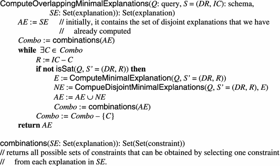

  

  Algorithm for computing overlapping minimal explanations

• Remove $Ic_{1}, Ic_{3}, Ic_{7}$

• Remove $Ic_{1}, Ic_{4}, Ic_{6}$

• $\ldots$

• Remove $Ic_{2}, Ic_{5}, Ic_{7}$

• Remove $Ic_{1}, Ic_{3}, Ic_{4}, Ic_{6}$

• Remove $Ic_{1}, Ic_{3}, Ic_{4}, Ic_{7}$

• Remove $Ic_{2}, Ic_{3}, Ic_{4}, Ic_{6}$

• Remove $Ic_{2}, Ic_{3}, Ic_{4}, Ic_{7}$

• Remove $Ic_{1}, Ic_{3}, Ic_{5}, Ic_{6}$

• $\ldots$

• Remove $Ic_{2}, Ic_{4}, Ic_{5}, Ic_{7}$

For each of these combinations, we repeat the query satisfiability check on the remaining constraints. If the query is now satisfiable, then the current combination does not lead us to finding any new explanation, and we simply try the next one. Otherwise, we minimize the approximated explanation retuned by the $\mathrm{{CQC}}_\mathrm{E}$, and we get a new minimal explanation that overlaps with the ones we already have. Then, we extend the set of combinations above with the constraints in the new explanation and repeat the process. The second stage ends when all the combinations have been explored.

5 Related work

In this section, we review current tools for checking the correctness of a UML/OCL conceptual schema and related work on computing explanations.

5.1 Tools for checking the correctness of a UML/OCL conceptual schema

There exist several tools for checking the correctness of a UML/OCL conceptual schema. We review the most relevant ones in this section. It is worth mentioning that none of these tools is able to provide the kind of explanations that we do.

One of the best-known tools to validate UML/OCL conceptual schemas is USE [16]. This tool allows the designer to provide an instantiation of the schema and to check whether it satisfies the OCL constraints. USE may also trace and debug the validity of an expected theorem (i.e., an OCL constraint) within a given instantiation provided by the designer [7], but it does not tell the user whether there are other causes (i.e., explanations) for the same problem as AuRUS does. USE behaves as model checking since it may determine whether a constraint is violated, but it is not able to invent new instances that could complement the given test case to make it valid if it is not. Note that, although a scripting language for snapshot generation (i.e., instance generation) is defined in [16], the actual generation of schema instances requires that the user writes a program using this language; a program that, when executed, produces a schema instance. This differs from our approach in the sense that AuRUS is able to automatically generate instances given only the schema and the property to be tested, without the user having to provide them neither manually nor via a script program. Regarding the supported language, AuRUS restricts the subset of OCL to expressions built using the operators indicated in Sect. 2. USE does not have this restriction and supports full OCL.

A similar functionality is provided by the ITP/OCL tool [11], which supports automatic validation of UML class diagrams with respect to OCL constraints. This tool is also able to check whether a given instantiation satisfies the OCL constraints, but it is not able to invent new instances when it does not. The implementation of ITP/OCL is directly based on the equational implementation of UML/OCL class diagrams. This tool does not restrict the supported OCLlanguage.

The UMLtoCSP tool [8] is aimed at the formal verification of UML/OCL schemas using constraint programming. This tool is able to verify typical properties such as satisfiability, class liveliness or non-redundancy of integrity constraints. These properties are similar to some of the checks performed by AuRUS in the sense that they are based on the properties defined in [12]. A major difference between UMLtoCSP and AuRUS is that the former does not provide any kind of explanation when the tested property does not hold (in the case when the property holds, both tools provide an instance of the schema that illustrates that fact). Moreover, completeness is not always guaranteed by UMLtoCSP since it restricts the domains of the variables in order to guarantee decidability and this may imply failing to find an existing solution. Regarding the supported OCL operators, UMLtoCSP is less restrictive than AuRUS; in particular, it supports arithmetic operations and comparisons while AuRUS supports only comparisons.

The HOL-OCL system [6] is an interactive proof environment for UML and OCL. It provides several derived proof calculi that allow the formal derivations establishing the validity of UML/OCL formulas. This system allows the user to reason over the schema; however, it is the user who has to guide the construction of the corresponding proofs, while AuRUS performs its checks automatically. It is not clear, however, how some checks that AuRUS is able to perform can be done in HOL-OCL. In particular, we do not see an easy way to simulate AuRUS’ interactive validation check. This check is parameterized by the user with particular data, in such a way that the existence of a consistent instance of the schema that includes this data is tested; however, proofs in HOL-OCL refer to elements of the schema and not data. The output produced by the two systems is entirely different; while HOL-OCL produces a formal proof for the tested property, AuRUS provides either an instance of the schema that exemplifies the satisfaction of the property or highlights the constraints responsible for its failure. Also, it is worth noting that a formal proof that shows the failure of a property may not be pinpointing all the possible causes of the problem, whereas AuRUS feature of computing all minimal explanations does. HOL-OCL does, however, support all standard OCL operators, while AuRUS restricts them to a particular subset.

The OCLE environment [10] is a tool for checking the consistency of UML models. The checks provided by this tool allow ensuring the consistency of UML models as defined by means of well-formedness rules specified in OCL. This kind of validation is complementary to the one we propose in this paper since we assume that the model to validate already satisfies such well-formedness rules.

Wahler et al. [35] propose consistency checking rules for constraints patterns. A constraint pattern is a parameterized constraint expression that can be instantiated to produce specific constraints. The check is syntax-based, and it can thus be done in polynomial time. The user gets pairs of pattern instances that can potentially contradict each other, but an alternative approach is required to check whether they are really contradictory. Wahler et al. also survey different notions of consistency for UML/OCL schemas. AuRUS’ test that checks if all classes are lively corresponds to the notion of class consistency in [35].

5.2 Computing explanations

Our notion of explanation is related to that of Minimal Unsatisfiable Subformula (MUS) in the propositional SAT field [17] and to that of axiom pinpointing in Description Logics [30]. In the next subsections, we review the most relevant works in these areas. We also review the relevant works that deal with explanations in the field of UML/OCL conceptual schemas.

5.2.1 Explanations in propositional SAT

The explanation of contradictions inside sets of propositional clauses has received a lot of attention during the last years. A survey of existing approaches to this problem can be found in [17]. The majority of these techniques rely on the concept of MUS in order to explain the source of infeasibility. A set of propositional clauses $U$ is said to be a MUS of a CNF (Conjunctive Normal Form) formula $F$ if (1) $U \subseteq F$, (2) $U$ is unsatisfiable and (3) $U$ cannot be made smaller without becoming satisfiable. Notice that what we call an explanation is basically the same as a MUS; the difference is that instead of propositional clauses we have schema constraints and mapping assertions.

It is well known that there may be more than one MUS for a single CNF formula. The most efficient methods for the computation of all MUSes are those that follow the hitting set dualization approach—see the algorithm [3] and the algorithms [18, 19]. The hitting set dualization approach is based on a relationship that exists between MUSes and CoMSSes, where a CoMSS is the complementary set of a MSS, and a MSS is a Maximal Satisfiable Subformula defined as follows. A set of clauses $S$ is a MSS of a formula $F$ if (1) $S \subseteq F$, (2) $S$ is satisfiable and (3) no clause from $F$ can be added to $S$ without making it unsatisfiable. The relationship between MUSes and CoMSSes is that they are “hitting set duals” of one another, that is, each MUS has at least one clause in common with all CoMSSes (and is minimal in this sense), and vice versa. For example, assume that F is an unsatisfiable CNF formula with 6 clauses (denoted c1–c6) and that it has the following set of MSSes and CoMSSes (example taken from [17]):

$$\begin{aligned} \begin{array}{l} \mathrm{{MSSes}}: \{\mathrm{{c}}1, \mathrm{{c}}2, \mathrm{{c}}3, \mathrm{{c}}5, \mathrm{{c}}6\}, \{\mathrm{{c}}2, \mathrm{{c}}3, \mathrm{{c}}4, \mathrm{{c}}6\}, \{\mathrm{{c}}3, \mathrm{{c}}4, \mathrm{{c}}5\},\\ \quad \{\mathrm{{c}}2, \mathrm{{c}}4, \mathrm{{c}}5\}\\ \mathrm{{CoMSSes}}: \{\mathrm{{c}}4\}, \{\mathrm{{c}}1, \mathrm{{c}}5\}, \{\mathrm{{c}}1, \mathrm{{c}}2, \mathrm{{c}}6\}, \{\mathrm{{c}}1, \mathrm{{c}}3, \mathrm{{c}}6\}\\ \end{array} \end{aligned}$$

The corresponding set of MUSes would be the following:

$$\begin{aligned} \begin{array}{llll} \mathrm{{MUSes}}:&\{\mathrm{{c}}2, \mathrm{{c}}3, \mathrm{{c}}4, \mathrm{{c}}5\},&\{\mathrm{{c}}1, \mathrm{{c}}4\},&\{\mathrm{{c}}4, \mathrm{{c}}5, \mathrm{{c}}6\} \end{array} \end{aligned}$$

Notice that each MUS has indeed an element in common with each CoMSS, and that removing any element from a MUS would invalidate this property.

In order to find all MUSes, the algorithms that follow the hitting set dualization approach start by finding all MSSes, then compute the CoMSSes, and finally find the minimal hitting sets of these CoMSSes. The intuition of why this approach is more efficient than finding the MUSes directly is the fact that, in propositional SAT, finding a satisfiable subformula can be done in a more efficient way than finding an unsatisfiable one, mainly thanks to the use of incremental SAT solvers. Moreover, the problem of finding the minimal hitting sets is equivalent to computing all minimal transversals of a hypergraph; a well-known problem for which many algorithms have been developed.

The problem of applying hitting set dualization in our context is that, to our knowledge, there is no incremental method for query satisfiability checking, and, in particular, it is not clear how to make the CQC method incremental (that could be a topic for further research). Therefore, there is no advantage in going through the intermediate step of finding the MSSes, and finding the MUSes directly becomes the more efficient solution. This intuition is confirmed by the experiments we have conducted [27] to compare the techniques discussed in Sect. 4 with the algorithm of Bailey and Stuckey [3].

Since in the worst case the number of MUSes may be exponential w.r.t. the size of the formula, computing all MUSes may be costly, especially when the number of clauses is large. In order to combat this intractability, Liffiton and Sakallah [19] propose a variation of their hitting set dualization algorithm that does not compute all CoMSSes neither all MUSes, but a subset of them. This goes on the same direction that the first stage of the algorithm for finding all minimal explanation from Sect. 4.2, which is more than a mere intermediate step in the process of finding all explanations. It provides a maximal set of minimal explanations with only a linear number of calls to the $\mathrm{{CQC}}_\mathrm{E}$ method. The idea is to relax completeness so the user can obtain more than one explanation without the exponential cost of finding all of them.

Also because of this intractability, many approaches to explain infeasibility of Boolean clauses focus on the easier task of finding one single MUS. The two main approaches are the constructive [32] and the destructive [4]. The constructive approach considers an initial empty set of clauses $F^{\prime }$. It keeps adding clauses from the given formula $F$ to the set $F^{\prime }$ while $F^{\prime }$ is satisfiable. When $F^{\prime }$ becomes unsatisfiable, the last added clause $c$ is identified as part of the MUS. The process is iterated with $F^{\prime }-\{c\}$ as the new formula $F$ and $\{c\}$ as the new set $F^{\prime }$. The process ends when $F^{\prime }$ is already unsatisfiable at the beginning of an iteration, which means that $F^{\prime }$ is a MUS.

The destructive approach considers the whole given formula and keeps removing clauses until the formula becomes satisfiable. When that happens, the last removed clause is identified as part of the MUS. The process is iterated with the identified and remaining clauses as the new initial formula. The process ends when no new clause is identified.

The computation of one MUS relates with the algorithm for minimizing an explanation from Sect. 4.1, which is aimed at computing one minimal explanation (from the approximated explanation provided by the $\mathrm{{CQC}}_\mathrm{E})$. The minimization algorithm applies the destructive approach to our context and combines it with the $\mathrm{{CQC}}_\mathrm{E}$ method. The idea is to take advantage of the fact that the $\mathrm{{CQC}}_\mathrm{E}$ does not only check whether a given query is satisfiable, but also provides an approximated explanation (i.e., not necessarily minimal) when is not. The destructive approach is the one that is best combined with the $\mathrm{{CQC}}_\mathrm{E}$ since it is expected to perform a lot of satisfiability tests with negative result. Each time a constraint is removed, and the tested query is still unsatisfiable w.r.t. the remaining constraints, the $\mathrm{{CQC}}_\mathrm{E}$ will provide an approximated explanation in such a way that in the next iteration of the destructive approach we will be able to remove all remaining constraints that do not belong to the approximated explanation. This way, the number of calls that the minimization algorithm makes to the $\mathrm{{CQC}}_\mathrm{E}$ decreases significantly. Moreover, since the minimization algorithm is reused by the algorithm that finds all minimal explanations (Sect. 4.2), we can benefit from this combination of the minimization algorithm and $\mathrm{{CQC}}_\mathrm{E}$ not only when we are interested in computing one explanation, but also when computing either a maximal set of disjoint explanations or all the possible explanations.

Given that computing one single MUS still requires multiple calls to the underlying satisfiability method, some approaches consider the approximation of a MUS a quicker way of providing the user with some useful insight into the source of infeasibility of the formula. Zhang and Malik [37] propose a glass-box approach that makes use of a resolution graph that is built during the execution of the SAT solver. The resolution graph is a directed acyclic graph in which each node represents a clause and the edges represent a resolution step. An edge from a node A to a node B indicates that A is one of the source clauses used to infer B via resolution. The root nodes are the initial clauses, and the internal nodes are the clauses obtained via resolution. In order to obtain an approximated MUS, the root nodes that are ancestors of the empty clause are considered. Such a MUS is approximated since it is not guaranteed to be minimal. The drawback of this approach is the size of the resolution graph, which may be very large; actually, in most cases, the resolution graph is stored in a file on disk. Besides the storage problems, the additional step that is required to obtain the approximated MUS from the resolution graph may also introduce a significant cost given the necessity of exploring the file in a reverse order.

5.2.2 Explanations in description logics

Axiom pinpointing is a technique introduced by Schlobach and Cornet [30] as a non-standard reasoning service for the debugging of Description Logic terminologies. The idea is to identify those axioms in a given DL terminology that are responsible for the unsatisfiability of its concepts, which is similar to the concept of MUSes in the SAT field and to our notion of explanations. They define a MUPS (Minimal Unsatisfiability-Preserving Sub-TBox) as a subset $T^{\prime }$ of a terminology $T$ such that a concept $C$ from $T$ is unsatisfiable in $T^{\prime }$, and removing any axiom from $T^{\prime }$ makes $C$ satisfiable.

Schlobach and Cornet propose a glass-box approach to calculate all the MUPSes for a given concept with respect to a given terminology. The algorithm works for unfoldable ALC terminologies [22] (i.e., ALC terminologies whose axioms are in the form of $C \sqsubseteq D$, where $C$ is an atomic concept and $D$ contains no direct or indirect reference to $C$), although it has been extended to general ALC terminologies in [21]. The idea is to extend the standard tableau-like procedure for concept satisfiability checking, and decorate the constructed tableau with the axioms that are relevant for the closure of each branch. After the tableau has been constructed and the tested concept found unsatisfiable, an additional step is performed, which applies a minimization function on the tableau (it can also be applied during the construction of the tableau) and uses its result (a Boolean formula) to obtain the MUPSes. The MUPSes will be the prime implicants of the minimization function result, i.e., the smallest conjunctions of literals that imply the resulting formula. Comparing with the $\mathrm{{CQC}}_\mathrm{E}$, the main difference is that the two approaches have different goals; while our method is aimed at providing one approximated explanation without increasing the running time, the algorithm of Schlobach and Cornet provides all the exact MUPS, but that requires and additional exponential cost.

A black-box approach to the computation of MUPSes is presented in [31]. Since it makes use of an external DL reasoner, it can deal with any class of terminology for which a reasoner exists. The algorithm uses a selection function to heuristically choose subsets of axioms of increasing size from the given terminology. The satisfiability of the target concept is checked against each one of these subsets. The approach is sound, but, however, not complete, i.e., it does not guarantee that all MUPSes are found. In this sense, it is similar to the first stage of the algorithm for finding all minimal explanations from Sect. 4.2, which produces an incomplete but sound set of minimal explanations.

Another way of explaining the result of the different reasoning tasks in Description Logics is explored by Borgida et al. [5]. Their notion of explanation is different from ours in the sense that they consider an explanation to be a formal proof, which can be presented to the user following some presentation strategy (e.g., tree-shaped proofs). They propose a set of inference rules for each reasoning task commonly performed in DL-Lite [9]. Then, a proof can be constructed from the premises by means of using the corresponding set of inference rules. As future research, it would be interesting to study how these proof-like explanations can be combined with ours. The motivation would be that highlighting the constraints responsible for the result of the test may not be enough to fully understand what the problem is, i.e., it may not be clear what the precise interaction between the highlighted elements is, especially if the constraints are complex. In this situation, providing some kind of proof that illustrates how these elements relate might be very useful.

5.2.3 Explanations in UML/OCL schemas

Wille et al. presented in [36] an approach for automatically checking the consistency of an UML/OCL model (i.e., a conceptual schema) and determining contradiction candidates. This concept of contradiction candidate is related to our notion of explanation since it pinpoints a small subset of the original schema which explains the conflict. They compute the contradiction candidates in two phases. First, they focus on the UML part of the schema. If a contradiction is found, they provide the corresponding contradiction candidates. Otherwise, the OCL part of the schema is examined, and its contradiction candidates computed. They use two different solvers, one for each phase: a Linear Integer Arithmetic solver for the UML phase and a Bit-Vector Logic solver for the OCL phase. Comparing with our approach, the main difference is that we reason over the UML and OCL parts at the same time. This makes a difference, since it allows us to provide explanations that relate both parts of the schema, i.e., it may be that a test fails because of a contradiction that involves not only UML elements or only OCL elements but both of them.

Soeken et al. introduce in [33] at bit-vector encoding for OCL data types, including sets and bags, which enables the verification of UML/OCL models using a SAT solver. In particular, they address the verification of two properties: consistency of the schema (i.e., whether there is a consistent instance of the schema), and reachability of an OCL expression (i.e., whether there is an instance in which the OCL expression is true or returns a non-empty result), but they restrict the number of objects in the instance of the schema to be a particular number. From the point of view of explanations, their approach provides a witness that exemplifies the satisfaction of the tested property, but they do not provide any kind of explanation for the negative case (i.e., when the tested property does not hold). In this sense, their notion of witness corresponds to our notion of (counter)example provided by the AuRUS tool, but not to our notion of explanation.

6 Conclusions and further work

The AuRUS tool is able to check the (in)correctness of a UML/OCL conceptual schema by providing the designer with several properties both to verify and to validate the schema. AuRUS reasons directly from the schema and is able to determine whether each one of these properties is satisfied by at least one of the possible instances of the schema.

The conceptual schema can be specified in ArgoUML, an open source CASE tool, since the XMI file of the schema automatically generated by ArgoUML can be directly uploaded to AuRUS to perform the analysis. AuRUS is available as a web application at folre.essi.upc.edu.

Verification properties include classical properties such as class liveliness or non-redundancy of a constraint, but also additional properties such as correctness of minimum and maximum cardinalities or correctness of incomplete or overlapping hierarchies. AuRUS incorporates also some predefined properties for validation such as missing identifiers, missing irreflexive constraints or missing inclusion or exclusion path constraints. Validation may also be achieved by allowing the designer to freely check for all properties he may find relevant to assess compliance with the requirements. To our knowledge, no other tool allows for such a wide spectrum of verification and validation properties.

When a property is satisfied, AuRUS also provides a sample instantiation proving the property. When it is not, AuRUS delivers an explanation for such unsatisfiability, i.e., a set of integrity constraints which is in contradiction with the property. This feedback is very relevant for the designer to be able to assess whether the schema actually complies with the requirements and to fix the errors encountered during the analysis of the schema.

Despite the theoretically high computational cost of performing such kind of analysis in UML/OCL conceptual schemas (due to the high expressivity of both languages), our experience shows that AuRUS behaves quite efficiently for conceptual schemas like the one considered in this paper, where the maximum time we have required to check some property is 8.5 s.

As further work, we plan to extend our techniques to validate not only the structural part of the schema but also its behavioral part, i.e., the set of operations that can be applied to the schema and that are gathered as a result of the requirements engineering phase.

References

Abiteboul, S., Hull, R., Vianu, V.: Foundations of Databases, vol. 8. Addison-Wesley, Reading (1995)
ArgoUML: http://argouml.tigris.org/ (2012)
Bailey, J., Stuckey, P.J.: Discovery of minimal unsatisfiable subsets of constraints using hitting set dualization. Practical Aspects of Declarative Languages. Lecture Notes in Computer Science, vol. 3350, pp. 174–186 (2005)
Bakker, R.R., Dikker, F., Tempelman, F., Wognum, P.M.: Diagnosing and solving over-determined constraint satisfaction problems. Int. Joint Conf. Artif. Intell. 13, 276–276 (1993)
Borgida, A., Calvanese, D., Rodriguez-Muro, M.: Explanation in the dl-lite family of description logics. On the Move to Meaningful Internet Systems: OTM 2008. Lecture Notes in Computer Science, vol. 5332, pp. 1440–1457 (2008)
Brucker, A. D., Wolff, B.: HOL-OCL: A formal proof environment for UML/OCL. In: Fiadeiro, J.L., Inverardi, P. (eds.) Fundamental Approaches to Software Engineering. Lecture Notes in Computer Science, vol. 4961, pp. 97–100. Springer, Berlin, Heidelberg (2008)
Brüning, J., Gogolla, M., Hamann, L., Kuhlmann, M.: Evaluating and debugging OCL expressions in UML models. In: Brucker, A.D., Julliand, J. (eds.) Tests and Proofs, vol. 7305, pp. 156–162. Springer, Berlin (2012)
Cabot, J., Clarisó, R., Riera, D.: UMLtoCSP: a tool for the formal verification of UML/OCL models using constraint programming. In: Proceedings of the Twenty-Second IEEE/ACM International Conference on Automated Software Engineering, ASE ’07, pp. 547–548. New York, NY, USA (2007)
Calvanese, D., De Giacomo, G., Lembo, D., Lenzerini, M., Rosati, R.: Tractable reasoning and efficient query answering in description logics: the DL-Lite family. J. Autom. Reason. 39(3), 385–429 (2007)
Chiorean, D., Pasca, M., Cârcu, A., Botiza, C., Moldovan, S.: Ensuring UML models consistency using the OCL environment. Electron. Notes Theor. Comput. Sci. 102(November), 99–110 (2004)
Clavel, M., Egea, M.: ITP/OCL: a rewriting-based validation tool for UML+OCL static class diagrams. In: Johnson, M., Vene, V. (eds.) Algebraic Methodology and Software Technology, vol. 4019, pp. 368–373. Springer, Berlin (2006)
Decker, H., Teniente, E., Urpí, T.: How to tackle schema validation by view updating. In: Proceeding of the 5th International Conference on Extending Database Technology (EDBT), pp. 535–549 (1996)
EinaGMC Project: http://guifre.lsi.upc.edu/eina_GMC/ (2011)
Farré, C., Teniente, E., Urpí, T.: Checking query containment with the CQC method. Data Knowl. Eng. 53(2), 163–223 (2005)
Gogolla, M., Richters, M.: Expressing UML class diagrams properties with OCL. In: Object Modeling with OCL, Lecture Notes in Computer Science, vol. 2263, pp. 85–114 (2002)
Gogolla, M., Bohling, J., Richters, M.: Validating UML and OCL models in USE by automatic snapshot generation. Softw. Syst. Model. 4(4), 386–398 (2005)
Grégoire, É., Mazure, B., Piette, C: On approaches to explaining infeasibility of sets of Boolean clauses. In: 20th IEEE International Conference on Tools with Artificial Intelligence, 2008. ICTAI’08 vol. 1, pp. 74–83 (2008)
Liffiton, M.H., Sakallah, K.A.: On finding all minimally unsatisfiable subformulas. In: Theory and Applications of Satisfiability Testing, Lectur Notes in Computer Science, vol. 3569, pp. 173–186 (2005)
Liffiton, M.H., Sakallah, K.A.: Algorithms for computing minimal unsatisfiable subsets of constraints. J. Autom. Reason. 40(1), 1–33 (2008)
Lloyd, J.W., Topor, R.W.: Making prolog more expressive. J. Logic Program. 1(3), 225–240 (1984)
Meyer, T., Lee, K., Booth, R., Pan, J.Z.: Finding maximally satisfiable terminologies for the description logic ALC. In: Proceedings of the National Conference on Artificial Intelligence, vol. 21, p. 269 (2006)
Nebel, B.: Terminological reasoning is inherently intractable. Artif. Intell. 43(2), 235–249 (1990)
OMG: (2011a). http://www.omg.org/spec/UML/
OMG: 2011b OCL http://www.omg.org/spec/OCL/
Queralt, A., Rull, G., Teniente, E., Farré, C., Urpí, T.: AuRUS: automated reasoning on UML/OCL schemas. In: Conceptual Modeling—ER 2010. http://www.springerlink.com/content/x15v9q081x602204/ (2010)
Queralt, A., Teniente, E.: Verification and validation of UML conceptual schemas with OCL constraints. ACM Trans. Softw. Eng. Methodol. 21(2), 13 (2012)
Rull, G.: Validation of mappings between data schemas. PhD Thesis. Universitat Politècnica de Catalunya (2011). http://hdl.handle.net/10803/22679
Rull, G., Farré, C., Teniente, E., Urpí, T.: Computing explanations for unlively queries in databases. In: Proceedings of the Sixteenth ACM Conference on Conference on Information and, Knowledge Management, pp. 955–958 (2007)
Rull, G., Farré, C., Teniente, E., Urpí, T.: Providing explanations for database schema validation. In: Database and Expert Systems Applications, pp. 660–667 (2008)
Schlobach, S., Cornet, R.: Non-standard reasoning services for the debugging of description logic terminologies. In: International Joint Conference on Artificial Intelligence vol. 18, pp. 355–362 (2003)
Schlobach, S., Huang, Z., Cornet, R., van Harmelen, F.: Debugging incoherent terminologies. J. Autom. Reason. 39(3), 317–349 (2007)
De Siqueira, J.L., Puget, J.F.: Explanation-based generalisation of failures. In: Proceedings of ECAI vol. 88, pp. 339–344 (1988)
Soeken, M., Wille, R., Drechsler, R.: Encoding OCL data types for SAT-based verification of UML/OCL models. In: Proceedings of the 5th International Conference on Tests and Proofs, TAP’11. pp. 152–170. Springer-Verlag, Berlin, Heidelberg (2011)
Ullman, J.D.: Principles of Database and Knowledge-Base Systems, vol. 2. Computer Science Press, New York (1989)
Wahler, M., Basin, D.A., Brucker, A.D., Koehler, J.: Efficient analysis of pattern-based constraint specifications. Softw. Syst. Model. 9(2), 225–255 (2010)
Wille, R., Soeken, M., Drechsler, R.: Debugging of inconsistent UML/OCL models. In: Design, Automation Test in Europe Conference Exhibition (DATE) 2012, pp. 1078–1083 (2012)
Zhang, L., Malik, S.: Validating SAT solvers using an independent resolution-based checker: practical implementations and other applications. In: Design, Automation and Test in Europe (DATE). pp. 10880–10885 (2003)
Acknowledgments
Our thanks to Lluís Munguía and Xavier Oriol, for their valuable help in the development of this tool. This work has been partly supported by Ministerio de Ciencia and Tecnología under TIN2011-24747, TIN2008-00444, Grupo Consolidado, and the FEDER funds.
Author information
Authors and Affiliations
Corresponding author
Additional information
Communicated by Prof. Tony Clark.
Rights and permissions
About this article
Cite this article
Rull, G., Farré, C., Queralt, A. et al. AuRUS: explaining the validation of UML/OCL conceptual schemas. Softw Syst Model 14, 953–980 (2015). https://doi.org/10.1007/s10270-013-0350-8
Received:
Revised:
Accepted:
Published:
Issue Date:
DOI: https://doi.org/10.1007/s10270-013-0350-8