
Abstract
In this paper, we use the unstructured grid model SCHISM to simulate the thermohydrodynamics in a chain of baroclinic, interconnected basins. The model shows a good skill in simulating the horizontal circulation and vertical profiles of temperature, salinity, and currents. The magnitude and phases of the seasonal changes of circulation are consistent with earlier observations. Among the mesoscale and subbasin-scale circulation features that are realistically simulated are the anticyclonic coastal eddies, the Sebastopol and Batumi eddies, the Marmara Sea outflow around the southern coast of the Limnos Island, and the pathway of the cold water originating from the shelf. The superiority of the simulations compared to earlier numerical studies is demonstrated with the example of model capabilities to resolve the strait dynamics, gravity currents originating from the straits, high-salinity bottom layer on the shallow shelf, as well as the multiple intrusions from the Bosporus Strait down to 700 m depth. The warm temperature intrusions from the strait produce the warm water mass in the intermediate layers of the Black Sea. One novel result is that the seasonal intensification of circulation affects the interbasin exchange, thus allowing us to formulate the concept of circulation-controlled interbasin exchange. To the best of our knowledge, the present numerical simulations, for the first time, suggest that the sea level in the interior part of the Black Sea can be lower than the sea level in the Marmara Sea and even in some parts of the Aegean Sea. The comparison with observations shows that the timings and magnitude of exchange flows are also realistically simulated, along with the blocking events. The short-term variability of the strait transports is largely controlled by the anomalies of wind. The simulations demonstrate the crucial role of the narrow and shallow strait of Bosporus in separating the two pairs of basins: Aegean-Marmara Seas from one side and Azov-Black Seas from the other side. The straits of Kerch and Dardanelles provide sufficient interbasin connectivity that prevents large phase lags of the sea levels in the neighboring basins. The two-layer flows in the three straits considered here show different dependencies upon the net transport, and the spatial variability of this dependence is also quite pronounced. We show that the blocking of the surface flow can occur at different net transports, thus casting doubt on a previous approach of using simple relationships to prescribe (steady) outflow and inflow. Specific attention is paid to the role of synoptic atmospheric forcing for the basin-wide circulation and redistribution of mass in the Black Sea. An important controlling process is the propagation of coastal waves. One major conclusion from this research is that modeling the individual basins separately could result in large inaccuracies because of the critical importance of the cascading character of these interconnected basins.
1 Introduction
Straits like the Denmark Strait (~200 m deep and ~300 km wide) and the Strait of Gibraltar (~300 m deep and ~15 km wide) provide connections between large water bodies with different thermohaline characteristics, substantially impacting the dynamics of the Atlantic Ocean. The impact of narrower straits on the dynamics of interconnected basins is still insufficiently quantified. This is the case with many European straits, e.g., the Bosporus, the Great Belt, and others, which are from one to several kilometers wide. The water exchange in these straits is limited by the shallow depths (~30 m at places), and thus, they keep the hydrological characteristics of adjacent basins very different.
The limited knowledge of the straits’ role in the dynamics of the European seas is largely due to the incapability of existing structured grid models to accurately resolve the processes in narrow straits and in the connected basins at the same time. One possibility to overcome this difficulty is to use unstructured grid models. Although most of these models are used for 2D applications or for estuarine studies, recent developments demonstrate good performance of unstructured grid models in addressing ocean and coastal scales (Lermusiaux et al. 2013; Danilov 2013; Scholz et al. 2013). With the present research, we aim to make a first step forward in simulating the water exchange in a cascade of semi-enclosed basins of Azov Sea-Black Sea-Marmara Sea-Aegean Sea.
Among the European semi-enclosed basins, only the Mediterranean Sea belongs to the group of concentration basins, where the sum of precipitation and river runoff is smaller than the evaporation. The Black Sea and the Baltic Sea are the largest representatives of the European estuarine seas. The Baltic Sea is connected to the North Sea via three straits (the Little Belt, the Great Belt, and the Sound), while three straits (the Kerch, the Bosporus, and the Dardanelles) connect the Southern European estuarine seas to the Mediterranean (Stanev and Lu 2013), thus building a large natural cascade (Fig. 1). In these straits, as well as in some other similar small ocean straits, the net long-term mean transport is largely driven by the river runoff but is also modulated by wind and atmospheric pressure. A two-layer exchange, which is similar to the transport in tidal estuaries, dominates the straits’ dynamics, with upper-layer transport from the less to more saline basins and bottom-layer transport in the opposite direction. For many thousands years, this cascade continued up to the Aral Sea via the Caspian Sea (Georgievski and Stanev 2006), but this upper part of the cascade was one-layer flow (similar to the ones between mountain lakes).

Model area and bathymetry in log scale (2 means 102 m). Black boxes are the areas around Kerch, Bosporus, and Dardanelles Straits, which are magnified in Fig. 2. Geographic names, locations, and transect lines where analyses of model simulations are discussed are also given. White line shows the transect analyzed in Fig. 4c, d, and the red one shows the transect analyzed in Fig. 10. Symbol “A” overlays the start and end position of these two section lines. The latter section is seen with more details in Fig. 2b. One zonal and one meridional transects north of Bosporus used for analysis are shown with the black lines. Part of the trajectory of the float WMO-7900592 is shown with the purple line. The following notations have been used: LI Limnos Island, V Varna station, S Synop. The mouths of the following rivers are shown with numbers: 1 Sakarya, 2 Kizilirmak, 3 Rioni, 4 Kuban, 5 Don, 6 Dnieper, 7 Dniester, 8 Danube. The position of the Black Sea is shown as an inset in the upper-left corner
The water properties in the interconnected estuarine basins studied here are very different from each other. Salinity in the Azov Sea is about 10–12; in the Black Sea, it ranges from 17–18 at sea surface (river plumes excluded) to ~22.3 at the bottom; in the Marmara Sea, salinity increases from ~22 at the surface to more than 38 within only ~50-m-thick layer below the surface and changes very little further down the depths; and in the Aegean Sea, the vertical salinity gradient is much smaller. The huge salinity contrast between the individual basins is dynamically controlled by the interbasin exchange; the latter is responsible also for the sharp vertical thermohaline and chemical-biological stratification in the individual basins.
There are a number of observational and numerical modeling studies of the individual basins addressed here: Azov Sea (Matishov et al. 2008), Black Sea (Stanev 1990), and Marmara Sea (Beşiktepe et al. 1994; Chiggiato et al. 2012; Sannino et al. 2017). Observations and modeling in the straits have also been widely addressed in the literature, and the following references give just some examples: Kerch Strait (Ivanov et al. 2014), Bosporus (Oğuz and Sur 1989; Özsoy et al. 1998; Oğuz 2005; Jarosz et al. 2011; Ilıcak et al. 2009; Sözer and Özsoy 2017), and Dardanelles (Stashchuk and Hutter 2001; Kanarska and Maderich 2008; Jarosz et al. 2012, 2013). So far, there has been no effort to address the dynamics of these interconnected basins from the Azov Sea to the Aegean Sea in a single study using 3D numerical models. An attempt to simulate the circulation in the Azov Sea, Black Sea, and Marmara in a single model setup has been done by Stanev (2005); however, the horizontal resolution in this study was too coarse to realistically resolve the Bosporus; the Strait of Dardanelles was closed. Recently, Maderich et al. (2015) analyzed the seasonal and interannual variability of the water exchange in this strait system using a chain of linked two-layer hydraulic models.
The increase of available computational power and the improved realism of 3D baroclinic unstructured grid models (Zhang et al. 2016b) make the simulations of cascading basins feasible. In a recent study by Bajo et al. (2014), a finite-element baroclinic model has been set up (to our knowledge for the first time) for the Black Sea with a mesh resolution varying from 1.5 km near the coasts to ~10 km in the central Black Sea. This model had only 43,823 nodes and 83,938 triangular elements. Open boundaries at rivers and at the Bosporus were prescribed from monthly data, along with a relatively simple boundary condition for salinity. This study addressed the performance of the model only in a very small area around the Danube Delta. To the best of the authors’ knowledge, the second published application of an unstructured grid model for the Black Sea was by Zhang et al. (2016b). However, in their paper, only an illustration was given on the capabilities of the model to resolve the baroclinic instability in the Black Sea.
In the present study, we will describe the setup and demonstrate the performance of an unstructured grid model (Semi-implicit Cross-scale Hydroscience Integrated System Model (SCHISM), Zhang et al. 2016b) for the chain of cascading basins from the Azov to the Aegean Sea. It is not possible to address in one study all interesting physical aspects studied in the past that were published in several dozens of papers. Therefore, we will focus our analysis on processes that were inadequately or insufficiently addressed in the previous modeling work. Dynamics studied earlier will be presented in more general terms just to demonstrate the consistency of the present numerical simulations with the previous studies.
The paper is structured as follows. We present in Section 2 the physical characteristics of the studied region. The numerical model is presented in Section 3. Section 4 describes the results of numerical simulations with a focus on horizontal and vertical thermohaline patterns and circulation. Sections 5 and 6 describe the sea levels in the cascading basins and straits dynamics, respectively. The paper ends with a brief conclusion in Section 7.
2 Model area
2.1 Overall characteristics
The three cascading (estuarine) seas are very different from each other and unique in their own ways: the Sea of Azov is the world’s shallowest sea (shallower than the Ekman depth), the Black Sea is the world’s largest anoxic basin, and the Sea of Marmara, unlike the Black Sea, is ventilated down to the bottom by the denser inflow from the Aegean Sea, and therefore, it is oxic in the entire water column.
The Sea of Azov is a small (40,000 km3) basin with a very flat bottom. Its average depth is ~8 m and the maximum depth is 14.5 m. The largest rivers that flow into the Sea of Azov are the Kuban River and the Don River (4 and 5 in Fig. 1) with an annual runoff of ~40 km3/year. The sea level varies greatly, depending on the wind and the influx from rivers. The interannual range of the Azov Sea level is as large as 30 cm. Short-period oscillations may exceed 1 m. Wind waves combined with currents flowing counterclockwise along the coasts lead to the formation of complex coastal-morphological forms. Results from numerical simulations of the Azov Sea are documented by Ivanov and Shapiro (2004).
The main focus of this paper is the Black Sea, which is the largest basin in the studied cascade and has an area of 436,400 km2, a maximum depth of 2212 m, and a mean depth of ~1250 m. The net outflow of water of ~300 km3 per year through the Bosporus almost equals the river runoff because the evaporation and precipitation tend to cancel out each other. The Danube River (8 in Fig. 1) provides ~60% of this amount. The Marmara Sea water intrudes along the bottom of the Bosporus Strait and mixes with the Black Sea water on the shelf. Because of the large mixing before reaching the continental slope, this water mass does not sink deeper than 600–700 m (Özsoy et al. 1993; Stanev et al. 2004). The decrease of oxygen flux carried by the mixed Marmara Sea water into the Black Sea with increasing depth and its vanishing below the ultimate sinking depth facilitate the formation of the Black Sea anoxic layer below 100–150 m. The outflow (here and further in this paper, we use the terms outflow and inflow when the water leaves or enters the Black Sea, respectively) in the Bosporus is a mixture of Black Sea surface water and water from the cold intermediate layer (CIL) that entrains Marmara Sea water. Because of its very low salinity, this water mass flows on the top of the more saline Mediterranean inflow. The numerical modeling of the Black Sea is reviewed by Stanev (2005) where an extensive list of publications can be found.
The Sea of Marmara is an inland sea connected to the Black Sea via the Bosporus Strait and to the Aegean Sea via the Dardanelles Strait. It has an area of 11,350 km2 with the greatest depth reaching 1370 m. The river runoff into this sea is relatively small so the net flows in Bosporus and Dardanelles do not differ much. The Sea of Marmara can be considered as a mixing zone between the Black Sea and the Mediterranean. There the surface water properties resemble those of the Black Sea surface water; the deep layers are filled with Aegean Sea water. A sharp salinity interface (reaching ~1 per meter) at ~20 m separates these distinct water types. The mean upper-layer circulation which is largely driven by the southward flowing Bosporus jet is anticyclonic. The hydrography of the Marmara Sea has been reviewed by Beşiktepe et al. (1994) where an extensive list of publications has been provided. Chiggiato et al. (2012) presented the status of numerical modeling in the Marmara Sea.
2.2 The transports in the straits
Since at the heart of the present study is the numerical simulation of strait exchanges, a brief characterization of the Straits of Kerch, Bosporus, and Dardanelles is given below. The Strait of Kerch separates the Caucasian coast from the Crimea Peninsula (Fig. 2a). Its narrowest section is ~4 km wide between the Crimea Peninsula and the Island Tuzla. This is a very shallow strait, in particular in its eastern part (Taman Bay), which is separated from the navigation channel by Chushka Spit and Island Tuzla. The navigational Kerch-Yeni Kale channel is ~30 km long and only 120 m wide at its narrowest point; its shallowest depth is ~8 m. Altman (1991) described some concepts about the current system in the Kerch Strait based on observations from 1926 to 1980. Unlike the other two straits discussed in this paper, Kerch Strait had been relatively wide with several islands and spits inside, thus supporting pronounced horizontal circulation. This changed after 2003, in particular in the region of Taman Bay, when a spit (see Fig. 2a) was built. Since then, most of the exchange between the Azov Sea and the Black Sea is along the navigational channel. Analysis of numerical simulations of Fomin and Ivanov (2007) quantified the large difference between the two types of exchange before and after the spit was built. Observations analyzed by Ivanov et al. (2014) demonstrated that salinity in the strait varies between 12 and 18 depending on the direction of current. Upper layers are dominated by mixed Azov Sea water, while salinity in the deeper layers is closer to that of the Black Sea. Often a salinity front is observed in the middle of the navigation channel.

Bathymetry and numerical grid in the straits of Kerch (a), Bosporus (b), and Dardanelles (c). See the boxes in Fig. 1 for the location of the straits. The insets show the model grid in parts of the Bosporus Straits and Dardanelles. Some geographical names used in the text are also given. The transects where analyses of transport are shown are as follows: KSS and KSN in the Kerch Strait; BSN, BSC, and BSS in the Bosporus; and DA in the Dardanelles. Points used for other analyses are shown with pink dots
The Bosporus Strait (Fig. 2b) is about 30 km long, 0.6–3 km wide, and 28–110 m deep. The basic topographic forms that impact the current system are the constriction ~8 km north of Marmara exit and two sills (one at the southern exit and another one near the Black Sea exit). The mean sea-level difference between the two ends of the Bosporus is ~30 cm (Beşiktepe et al. 1994). The upper (low salinity) layer thickness is about 39 m near its northern end and about 14 m near its southern end but also exhibits large temporal variability. This variability is closely associated with the variability in the atmospheric forcing (Yuksel et al. 2008; Aydogan et al. 2010).
Ünlüata et al. (1990), Oğuz et al. (1990), and Oğuz (2005) supported the idea of a “maximal exchange” (Farmer and Armi 1986) and claimed that the hydraulic controls were caused by the mid-strait constriction (with a hydraulic jump south of it) and the sills. Gregg et al. (1999) claimed that the two-layer flow was subcritical, while in a more recent publication, Gregg and Özsoy (2002) emphasized on the role of friction. In addition, the flow in the Bosporus is also modulated by atmospheric forcing that may lead to flow blockages and reversals (Ünlüata et al. 1990; Özsoy et al. 1998; Yuksel et al. 2008). These controls could have a very fundamental role because they determine the basic characteristics of the exchange between the adjacent basins. Jarosz et al. (2011) presented a comprehensive analysis of data from bottom-mounted acoustic Doppler current profilers and temperature, conductivity, and pressure profiles over 5 months. These data reveal large temporal variations, which are more pronounced in the lower layer in the northern exit of Bosporus and in the upper layer in its southern part.
The Strait of Dardanelles (Fig. 2c) is about 61 km long and 1.2–7 km wide (Ünlüata et al. 1990) and its averaged depth is ~55 m (Jarosz et al. 2012). The two-layer exchange in this strait consists of a low-salinity outflow (mixed Black Sea water) in the surface layer and high-salinity Mediterranean water in the bottom layer flowing in from the Aegean Sea to the Sea of Marmara. The thickness of the upper layer decreases from the Marmara to the Aegean Sea, and water becomes more saline because of interfacial mixing (Ünlüata et al. 1990) and resultant recirculation back to the Aegean Sea. Oğuz and Sur (1989) reported a rapid transition of the interface depth south of the Nara Pass indicative of a hydraulic control. The lower layer flow is considered to be subcritical. These concepts are supported by the 2D modeling by Stashchuk and Hutter (2001). The long-term observations presented recently by Jarosz et al. (2012, 2013) indicated that on longer time scales (monthly or longer), the two layers showed little variability, but on synoptic time scales, the variations in both layers were pronounced with episodic flow reversals. These authors also reported a three-layer flow structure observed during short periods in the southern part of the straits.
3 The numerical model
3.1 Model description
SCHISM is a derivative product of the original semi-implicit Eulerian-Lagrangian finite-element (SELFE) model (Zhang and Baptista 2008), with many improvements described in Zhang et al. (2016b) and freely distributed under an open-source Apache v2 license (http://www.schism.wiki; last accessed January 2017). The model solves Reynolds-averaged Navier-Stokes equations along with transport of heat and salt. The model uses a hybrid finite-element and finite-volume approach. Its efficiency and robustness is mostly attributed to the implicit treatment of all terms that place stringent stability constraints (e.g., CFL) and the use of Eulerian-Lagrangian method for the momentum advection.
The version used in this study is hydrostatic with Boussinesq approximation. New development documented by Zhang et al. (2016b) includes a new advection scheme for the momentum equation, which uses an iterative smoother to reduce excess mass produced by higher-order kriging method; a viscosity formulation that works robustly for generic unstructured grids, filtering out spurious modes without introducing excessive numerical dissipation; and a higher-order, implicit, monotone transport solver (TVD2). The model uses mixed triangular-quadrangular elements in the horizontal dimension, as evidenced in the Bosporus and Dardanelles (Fig. 2b, c). The flexible vertical grid system LSC2 proposed in Zhang et al. (2015) enables model polymorphism and makes it possible to unify in a single model grid 1D/2DH/2DV/3D cells. As demonstrated by Zhang et al. (2016a), the vertical grid system is capable of maintaining sharp stratification in estuarine basins (e.g., the Baltic Sea). A key novelty of the model described by Zhang et al. (2016b) is that it resolves well the baroclinic instability, which makes it possible to use this model for oceanic areas where eddying processes play a dominant role. As it will be shown in the present study, the model is capable of simulating cross-scale processes (from straits scales to basin scales) in a seamless fashion.
The main digital elevation model (DEM) source we used is from the General Bathymetric Chart of the Oceans (GEBCO) Digital Atlas (IOC et al. 2003) with a resolution of 30 arcsec. Additionally, published data from Gökaşan et al. (2005, 2008), Oğuz et al. (1990), Özsoy et al. (2001, 2002), Ryabtsev (2005), Ilıcak et al. (2009), Ivanov et al. (2014), and Chiggiato et al. (2012) have been compared and digitized to construct bathymetry in the Azov Sea and Marmara Sea and in the straits, where the GEBCO data are too coarse. Finally, multiple data sources have been merged into a single unstructured DEM. The computational grid we generated has ~104K nodes and ~178K triangles/quadrangles with a minimum grid side length of ~80 m in the narrow areas of the Bosporus and Dardanelles Straits and ~400 m in the wider Kerch Straits (Fig. 2). An essentially uniform resolution of 3 km is used in the Black Sea in order to avoid possible distortion of eddies, which may affect processes associated with the baroclinic instability. The transition from the fine resolution in the straits to basin-scale resolution occurs mostly in the corresponding shelf zones. The vertical LSC2 grid consists of up to 53 levels in the deepest parts of the Black Sea, with an average number of 31.65 levels in the whole model domain. As indicated in Zhang et al. (2016b), no bathymetry smoothing is applied in spite of the very steep shelf breaks in the Black Sea; the flexibility of LSC2 grid allows a very faithful representation of the steep breaks.
The specification of bottom roughness is a general problem in ocean modeling due to lack of site-specific data for bottom sediment sizes over the entire model area. Therefore, bottom roughness is set to a constant value of 0.5 mm. This can be refined in future studies if respective data are available. The biharmonic viscosity is used as described by Zhang et al. (2016b). No explicit horizontal diffusivity is used as the higher-order solver is monotone by design and the vertical viscosity and diffusivity are calculated from the generic length-scale model (Umlauf and Burchard 2003) with a k-kl configuration.
3.2 Model integration
3.2.1 Initialization and forcing
Monthly climatological data of salinity and temperature are used to initialize the model in the Black Sea and Aegean Sea (http://marine.copernicus.eu/services-portfolio/access-to-products/; last accessed January 2017). The Marmara Sea is initialized with the hydrological data kindly provided by Chiggiato et al. (2012). Data from the atlas of Matishov et al. (2008) were used to initialize the Azov Sea. We consider these data as the best available estimates to initiate the model and so a dynamic equilibrium is established quickly. Straits are initialized as in lock exchange experiments: each half of the strait is filled with water from the closest basin. The adjustment in the straits to the forcing at their both sides is a very rapid process because of their low mechanical and thermohaline inertia due to shallow depths. Thus, the quasi-equilibrium model state is basically controlled by fluxes at the ocean surface, river runoff, and transport in the strait.
For atmospheric forcing, we use 6-hourly wind, atmospheric pressure, air temperature, and dew point temperature from the 0.2° ECMWF product. The 6-hourly 36-km CFSR product (http://rda.ucar.edu/datasets/ds093.1/; last accessed 23 March 2016) is used for downward long-wave and short-wave heat fluxes and precipitation. From these data, the wind shear stress and fluxes of sensible and latent heat are computed using bulk aerodynamic formulas. Freshwater fluxes from eight largest rivers, Danube, Dniepr, Rioni, Dniester, Sakarya, and Kizilirmak (discharging into the Black Sea) and Kuban and Don (discharging into the Azov Sea) are derived from monthly mean data (Kara et al. 2008). The locations of the river mouths are shown in Fig. 1.
The model has only one open boundary in the Aegean Sea. As shown by Volkov et al. (2016), this boundary is of utmost importance as a driver of exchange processes in the straits. We use the most adequate data available at this boundary such as daily mean values of elevation, horizontal velocity, salinity, and temperature taken from the Copernicus product (http://marine.copernicus.eu/; last accessed in January 2017), which are then interpolated at each time step onto the model grid. These data are considered as the best possible boundary conditions for our study because (1) they provide all the needed variables (including the ones down to the bottom) originating from one source, that is the data are dynamically consistent; (2) the used data product is based on assimilation of altimeter and profiling float data which guarantees the consistence with the observations; and (3) the product has been validated extensively.
In the paper, model validation is not organized as a separate section. Rather, analysis on consistency of model results is presented in different sections where individual processes have been addressed. In the Supplementary Material (SM1) section, a list for the model validation literature sources has been given along with an explanation to which variables these references are relevant.
3.2.2 Computational performance
After several sensitivity runs, a time step of 90 s was chosen. The frequency of output data was usually daily, but for specific analyses, 6-hourly outputs were also generated. On JURECA supercomputer in Julich, the model setup described above runs ~54 times faster than the real time when 144 MPI tasks are used. The results presented in the following cover a 2-year integration period starting in June 2008 after additional 2 years of spinup. According to the analysis of simulations, this spinup period is long enough to ensure a reasonable adjustment of model fields and realistic oceanographic conditions driving the straits exchange, which is central to this study. The specific model integration period was so chosen because extensive observations are available during this period to validate the model. The integration duration is sufficiently long to provide enough data to analyze variability from synoptic (atmosphere) to seasonal scales. Long-term climatic simulations are not subject of this study, as we focus mostly on the important physical processes and not on the long-term evolution of the cascading system. With the current model and computational resources available to us, it is not yet efficient enough to conduct such long-term experiments.
4 The numerically simulated circulation
4.1 Sea level and velocities
The simulated sea level in the Black Sea (Fig. 3a, d, g) agrees reasonably well with earlier analyses based on in situ observations (Oğuz et al. 1994; Oğuz and Besiktepe 1999; Zhurbas et al. 2004), satellite data (Korotaev et al. 2003), and numerical simulations (see Stanev 2005 for a review). The three snapshots used to illustrate the simulations reveal a pronounced slope of the sea level reaching ~0.3 m/50 km (e.g., on 08 October 2008, Fig. 3a). The magnitude of the Rim Current at sea surface is between 0.3 and 0.6 m/s, reaching in some areas values as high as 0.8 m/s. With increasing depth, velocities decrease showing a very good agreement with the results presented by Korotaev et al. (2006). The current at 200 m depth averaged over 1 year along the 1000-m isobaths is 6.9 cm/s. At the same depth, the average speed of the Rim Current reported by Korotaev et al. (2006) was 7 cm/s. The observed average speed of the Rim Current at 750 m was estimated by the same authors as 4.0 cm/s. The current simulated at 750 m averaged along the 1000-m isobaths and over 1 year is 5 cm/s. Considering the possible differences in the methods used in the above estimates, the relatively low signal-to-noise ratio, as well as the different periods of averaging, the comparison gives a proof that the model captures the basic vertical structure of the geostrophic current. We therefore conclude that the vertical gradient of geostrophic currents, which is proportional to the horizontal density gradient (thermal wind relationship), is accurately represented in the model. This guarantees a reasonable representation of the baroclinicity.

Sea level (a, d, g), SST (b, e, h) and relative vorticity at sea surface normalized by the Coriolis parameter (c, f, i). a–c Corresponds to 08 October 2008, d–f to 12 November 2008, and g–i to 22 January 2009. Note that the SST color bars have different ranges
The seasonal variations in the intensity of circulation (weak circulation in summer and more intense in winter) are very pronounced in the Black Sea and were attributed to the increase of the wind stress curl during winter (Stanev et al. 2000). In this work, the intensity of circulation is measured by the slope of sea level between the coastal and open-ocean areas. From the simulated data, we computed the averaged sea levels in the areas shallower than 500 m (i.e., coastal zone) and in the areas deeper than 2000 m (i.e., deep ocean). The difference between the intensities of winter and summer circulation (proportional to the coastal to open-ocean sea-level difference in the two seasons) measures the seasonal variability (1) of the geostrophic currents at sea surface. The annually averaged intensity (e.g., the annual mean surface geostrophic currents) is proportional to the annual mean coastal to open-ocean sea-level difference (2). The former (1) is about three times smaller than the latter (2), which is consistent with earlier analyses of Peneva et al. (2001), Stanev and Peneva (2002), and Stanev et al. (2003), and explains the relatively large role of the seasonal cycle in the Black Sea.
The higher position of sea surface in the coastal zone is accompanied by an anticyclonic circulation between the Rim Current and the coast (Fig. 3c, f, i) and is very well pronounced along the southern coast (e.g., Fig. 3c). The relative vorticity there is close to the planetary rotation.
The coastal and the subbasin eddies have been successfully simulated in earlier modeling studies (Staneva et al. 2001; Zhou et al. 2014). However, it was a priori not clear whether or not the unstructured grid models could simulate mesoscale dynamics. As demonstrated by Zhang et al. (2016b), the eddy-resolving capabilities of the model were only possible after a careful parameterization of the subgrid processes and appropriate numerics have been implemented. As mentioned in the model description, a uniform resolution of ~3 km is used in the Black Sea in order to avoid possible numerical distortion. This resolution is sufficient to resolve the mesoscale variability because the baroclinic Rossby radius in the Black Sea is ~15–20 km (Blokhina and Afanasyev 2003).
The major subbasin-scale features shown in Fig. 3 are the eddy in front of the Caucasian coast, which propagates into the direction of the Kerch Strait. This eddy has been reported earlier in the analyses of remote sensing and in situ data (Zatsepin et al. 2003, see their Fig. 5). Other prominent subbasin scale eddies are the Crimea and Batumi eddies (Fig. 3a, c, d, f). Note that because of their small scales and insufficient color resolution of sea-level maps, these mesoscale and subbasin features are sometimes better seen in the SST or in the vorticity plots; one example is the chain of coastal anticyclones along the southern coast in Fig. 3c (compare with Fig. 4.6 of Karimova 2011).
The dynamics of sea level is largely triggered by the changes in the atmospheric forcing; the response of the shallow Azov Sea gives one good example. The patterns in Fig. 3a, d are reminiscent of consequent surges with opposing sea levels at the two ends of this shallow sea. Another similar example is the positive sea-level anomaly in the western Black Sea in Fig. 3d, which is a short-lasting perturbation caused by changes of atmospheric pressure and wind. It propagates along the coast with a speed of up to ~2 m/s, eventually reaching the eastern Black Sea (see also Fig. 11 of Stanev and Beckers 1999 for the analysis of propagation of coastal waves in the Black Sea).
Since the present paper deals with several cascading basins, a major question arises as to what the approximate drop of sea levels along the chain Azov Sea-Black Sea-Marmara Sea-Aegean Sea is. Later in the text, the temporal dynamics of the basin mean sea levels will be analyzed in detail. Here we will only mention that during the time of integration, the mean drop of sea levels along the straits connecting adjacent basins is 1 cm (Kerch), 18 cm (Bosporus), and 10 cm (Dardanelles). The corresponding drops in the basin mean sea levels are 4 cm between the Azov Sea and Black Sea, 10–11 cm between the Black Sea and Marmara Sea, and 9–10 cm between the Marmara Sea and Aegean Sea.
The basin mean sea levels (and its standard deviations) in the Azov Sea, Black Sea, Marmara Sea, and Aegean Sea are 8.2 (10.4), 4.4 (9.2), −6.6 (10.7), and −15.5 (10.8) cm, respectively. The corresponding standard deviations estimated from the daily sea-level anomalies (MSLA) of SSALTO/DUACS as distributed by Aviso (www.aviso.oceanobs.com; last accessed in January 2017) are 8.6 cm (the Black Sea) and 8.1 cm (the Aegean Sea), which roughly support our model estimates. For the smaller basins of Azov and Marmara Seas, the altimeter data are not precise enough to allow such estimations. The differences between the basin mean sea levels of individual basins and the sea-level differences at the two ends of the respective straits are large, in particular for the case of the Black Sea and Marmara Sea. The dynamical role of this effect will be addressed later.
The standard deviations reported above are relatively small compared to the variability of the sea-level drops at the two ends of the individual straits (for the locations see the red points in Fig. 2a, c and locations A and Y in Fig. 2b). The corresponding numbers (rms) are 5–6 cm (Kerch Strait), 20–21 cm (Bosporus), and 10–11 cm (Dardanelles). These numbers are comparable to the mean values of the drops, thus demonstrating a vigorous variability triggered by external forcing and the response of individual basins to it. One has to also keep in mind that estimates of different authors vary largely in the literature. For the Dardanelles, the sea-level differences are 30–40 cm by Ünlüata et al. (1990) and Alpar and Yüce (1998), 7–8 cm by Möller (1928), and ~15 cm by Kanarska and Maderich (2008). An evidence for the correctness of our estimates is the comparison with Ssalto/Duacs data (www.aviso.oceanobs.com; last accessed in January 2017); both model and data show ~15-cm decrease in the Black Sea level during April 01, 2009–October 15, 2009, and ~15-cm increase in the Aegean Sea level during the same period.
The above estimates of sea-level differences between the individual basins and the respective changes of sea level in the straits give an overall presentation of the cascading in the considered interconnected system of seas. In order to understand the basic idea behind the analyses in the following sections, a comparison of the spatial contrasts of sea level inside each basin would be instructive. We take the Black Sea as the most important example, where the difference between the sea levels in the coastal and open-ocean areas is about 20–30 cm. This is comparable to the difference between the mean sea levels in the Black Sea and Marmara Sea and suggests that the sea level in the interior part of the Black Sea can be lower than the sea level in the Marmara Sea and even in some parts of the Aegean Sea (Fig. 3). Thus, a fundamental question arises: what is more important for the transport through the Bosporus, the sea-level difference associated with the estuarine character of the Black Sea (higher sea level in the basin with lower salinity), or the mechanical forcing (wind and atmospheric pressure driving the Black Sea circulation resulting in higher position of sea level in the coastal zone)? While it is well known that the wind can enhance or block the transport in the strait, depending on its direction and speed, it is still not clear whether the basin-wide circulation driven by wind (higher position of the sea level in the coastal zone, which is very pronounced in winter) could substantially affect the interbasin exchange. To the best of the authors’ knowledge, the impact of circulation and the associated higher sea level in the coastal zone on the exchange in the straits is novel and will be considered later in more detail.
4.2 Sea surface temperature
The SST patterns reveal a number of mesoscale elements of surface dynamics (Fig. 3b, e, h). The Caucasian water shows a westward propagation along the coast, reaching up to the Crimea Peninsula, where it is entrapped by the Sebastopol eddy (Fig. 3b). Such a propagation pattern is typical, as illustrated by the remote sensing observations of Zatsepin et al. (2003), see their Fig. 14) and Karimova (2011), see her Fig. 4.6). The comparison between Fig. 3b and c in the eastern part of the southern coast (between 36 E and 38 E) reveals several pairs of cyclonic and anticyclonic eddies, which have pronounced signatures in the small-scale SST pattern. The SST plots reveal more clearly than SSH plots the anticyclonic coastal eddies, as well as the system of currents and countercurrents along the western coast (Fig. 3b, e), which is also known from the in situ observations and analysis of numerical simulations (Trukhchev et al. 1985). The winter pattern (Fig. 3h) illustrates the extent and the propagation pathway of the cold water originating from the shelf, along with cold water intrusions into the open ocean. The simulated meanders and eddies in the frontal areas in the western Black Sea and south of the Kerch Strait are supported by the satellite data (e.g., Karimova 2011, Figs. 4.2 and 4.5; Zhou et al. 2014, Fig. 2).
The numerical simulations are also illustrative for the propagation patterns of surface water into the neighboring basins. As seen in Fig. 3e, the cooler water exiting into the Aegean Sea turns around the southern coast of the Limnos Island, similar to the Terra MODIS images acquired on July 11, 2003 (see http://eoimages.gsfc.nasa.gov/images/imagerecords/67000/67303/Turkey.A2003192.0900.1km.jpg; last accessed in January 2017). Because of the very shallow depth and thus low thermal capacity, the SST in the Azov Sea is very low in winter, reaching almost the atmosphere temperature. Therefore, the temperature signal from this sea is very strong; the cold intrusions from the Azov Sea clearly reveal the propagation pathway and mixing of this water with the Black Sea water (Fig. 3h, see also Karimova 2011, her Fig. 4.2).
4.3 Intrusions from the Bosporus Strait and intermediate water mass formation
In the basins considered here, the formation of water masses is controlled not only by the air-sea exchange, as is the dominant case in the world’s ocean, but also by the flows from the straits. The surface flows bring less salty water into the saltier basin; the bottom flow brings saltier water into the less salty basin. The major difference between the two-layer exchanges in the three straits is that, after exiting the straits, the bottom flow undergoes different propagation pathways. It reaches only very shallow depths in the (shallow) Azov Sea, intermediate depths in the Black Sea, and the bottom layers in the Marmara Sea. The Azov Sea is well ventilated because of its shallow depths; the relatively deep Marmara Sea is well ventilated because the deep inflow from the Aegean Sea through the Dardanelles reaches the bottom.
Recent observations using Argo floats can be used to validate the numerical simulations. Below, we use data from the float WMO-7900592, which was deployed on 15 December 2013 at 42.24 N. This device performed 79 cycles, many of which are in the close proximity of the Bosporus. Part of its trajectory where data are described below is shown in Fig. 1. The vertical temperature profiles (Fig. 4a) demonstrated that the inflow from the Bosporus (positive temperature anomalies) is usually detected between 150 and 300 m, but in exceptional cases, reaches more than 600 m. Such extreme depths have also been reported by Özsoy et al. (1993). On its way to the east, the float observed a number of temperature intrusions, which are seen in Fig. 4a as warm temperature anomalies. The latter are indicative of the warm water penetration and the mixing of this water with the Black Sea water. These intrusions are also identified in Fig. 4b by the red and dark-red patches appearing in the area of CIL (blue-colored area in the upper part of this figure), as well as in the deeper layers where temperature increases with depth.

Intrusions observed by the profiling float WMO-7900592 east of the Bosporus Straits during 2013–2014. a Vertical profiles of temperature. b Time versus depth temperature diagram. The trajectory of float, along which the data are presented in the two subfigures, is shown in Fig. 1
The numerics, spatial resolution, and boundary forcing used in the earlier numerical studies were unable to fully resolve the gravity currents originating from the straits. Simeonov et al. (1997), Stanev et al. (2001), and Özsoy et al. (2001) used a very fine horizontal resolution in the Bosporus inflow area, but their model was of the reduced-gravity type with a movable bottom layer. This model was not able to resolve the interleaving process. Parameterizations representing the entrainment and detrainment in a 3D circulation model of the Black Sea have been developed by Stanev et al. (2004), but the horizontal resolution used by these authors did not permit fully resolving the spatial patterns of gravity currents. In most of the earlier modeling works, the strait flows were prescribed, which did not allow the natural and forced variabilities to drive the inflow. In the present study, these drawbacks have been avoided and we will demonstrate some results from the numerical simulations with a focus on the Black Sea.
The analysis of the Bosporus inflow is presented below along one zonal (Fig. 5a) and one meridional (Fig. 5b) cross sections (see the black zonal and meridional lines in Fig. 1 for their positions). Figure 5c, d illustrates the intrusions along a section, which has been chosen such that it corresponds to the major pathway of propagation of Bosporus water (the white line north of Bosporus). In the inflow area, the contribution of temperature to buoyancy is smaller than that of salinity, and therefore, the temperature shown in these figures traces the penetration of intermediate waters well (Fig. 5b).

Penetration of the Marmara Sea water into the Black Sea. a Zonal (west at the left and east at the right) salinity and temperature cross sections on January 9, 2009. b The same but for a meridional section (south at the left and north at the right) on January 4, 2009. c, d Plotted along the red line in Fig. 1 near the exit of the Strait, which beyond the symbol “A” continues as a white line in the open-ocean (strait at the left and ocean at the right) on November 8, 2008, and November 26, 2008, respectively. The locations of cross sections are shown in Fig. 1
The specific times at which transects in Fig. 5 have been plotted were chosen so as to illustrate some basic intrusion patterns. One permanent characteristic of temperature in the Black Sea is the CIL with its core at about 80–150 m in the strait area. This layer indicates the propagation of Black Sea water in the direction of the Marmara Sea (Fig. 5c). The CIL shows different patterns in time and space. It is sometimes “split” by the warmer quasi-horizontal intrusions from the Marmara Sea (Fig. 5a). The simulated depth ranges of intrusions are consistent with the observations using Argo floats (Fig. 4). The multiple layering in the figures shows different appearances, demonstrating that the intrusions reach different depths under different inflow conditions.
The meridional cross section (Fig. 5b) demonstrates that the temperature intrusions are confined in a narrow zone (about 20–30 km) close to the coast; the more frequent intrusions occur in the depth range between 200 and 300 m, which is also consistent with the Argo observations. Some part of the warm water mixes with the Black Sea water and penetrates bellow 600 m following the continental slope in the form of gravity flow. This is illustrated in Fig. 5b by the “diffuse” warm temperature signal in the deeper levels. Our simulations confirm the observed penetration depths by Özsoy et al. (1993), as well as the estimations from the first numerical simulations of the deep intrusions of Stanev et al. (1997), but give much more detailed presentation of the dominant characteristics of water masses. The use of the LSC2 vertical grid system was instrumental in capturing the deep intrusion and gravity flows.
Depending upon the intensity of the inflow, the amount of warm water intruding into the intermediate layers varies substantially, as seen in the difference between Fig. 5c and d. These plots represent two different situations 2 weeks apart from each other. However, in both cases, the “preferred” depth of intrusions is about 200 m. With increasing distance from the strait, the axis of warm intermediate layer shallows to about 160 m (Fig. 5d).
The Bosporus inflow is easily detectable by higher salinity and temperature (Fig. 5d); the contrast with the Black Sea water decreases away from the strait. Although the salinity contrasts are less obvious than the temperature contrasts, several positive salinity anomalies appear at the positions where the temperature extrema occur (e.g., the mid-layer salinity maxima in Fig. 5a, b). Noteworthy is the fact that the shallower temperature maxima in Fig. 5a, b do not have clear salinity signatures. In most cases, the slope convection is well identified by the temperature maximum at the bottom of the straits (Fig. 5d). This can also be seen in the corresponding salinity pattern, but at shallower depths than the temperature intrusion. Below these depths, the propagation seems to be along isopycnal as demonstrated by Stanev et al. (2014).
4.4 Pathways of the inflows in the Black Sea
Because the present paper focuses mostly on the Black Sea, the flows contributing directly to the Black Sea hydrodynamics will be addressed here. These include the flow of low-salinity surface water from the Kerch Strait and the flow of high-salinity water from the Bosporus, which will be discussed separately.
4.4.1 The Bosporus inflow
The channel of Bosporus continues on the shallow shelf approximately in the same direction as between the two continents (Figs. 1, 2, and 6), and then, at about 29° 9′ 40″ E, 41° 19′ N, it turns to the North East (Okay et al. 2011). The simulations of Simeonov et al. (1997), Stanev et al. (2001), and Özsoy et al. (2001) demonstrated that the gravity currents are guided by this channel until they reach ~29° 6′ E, 41° 20′ N. Afterwards, the flow turns to the right (looking in the direction of its propagation) revealing an S-shaped pattern (Fig. 6). The individual figures show how variable the bottom flow is with time. At the beginning of the analyzed 1-week period from November 21, 2008, to November 28, 2008, the wind (directed to NE and with magnitudes of ~8 m/s) resulted in a relatively small inflow with a smooth S-shape. During November 22, 2008, the wind speed increased to 16 m/s. This change in the meteorological conditions resulted in a three-fold increase of the inflow into the Black Sea from ~15,000 m3/s on November 21 to 47,000 m3/s on November 23. The channel on the shelf was not able to accommodate this large inflow and a couple of overshoots (eastwards from the channel axis) appeared clearly on November 23, 2008 (Fig. 6b). Over time, the plume started to be “diluted” by the ambient water, and approached the continental slope where it plunged into the deeper layers. Its distinctive vertical structure is shown in the inset in Fig. 6d (at the location marked by the black circle in the same figure). The ability to simulate this vertical distribution, in particular the thin high-salinity bottom layer with the new LSC2 vertical grid, is a step ahead in comparison with some earlier simulations in this area (Simeonov et al. 1997; Stanev et al. 2001; Özsoy et al. 2001).

Bottom salinity during the inflow event in November 2008. White isoline is the 250-m isobath. The individual frames correspond to 00:00 GMT on a November 21, 2008; b November 23, 2008; c November 25, 2008; and d November 27, 2008. The inset in d shows vertical profiles of salinity in the location marked on the horizontal plot
Over most of the region shown in Fig. 6, the plume crosses the depth contours on the shallow shelf (e.g., the wider the shelf, the further the plume penetrates). The decoupling between the plume and the deep water beyond the continental slope persisted approximately along the 200-m isobath. These two water types (plume and deep water) are identified by the bottom-salinity maxima on the shelf and in the deep sea. This result manifests that the deeper penetration of the Bosporus inflow is rather intermittent; thus, the cascading of the saltier water can be considered as an extreme event. Such events happen during the times when the inflow overshoots the channel sides and takes the short path toward the deep canyons (Fig. 6b). During such extreme cases, the penetration depth of salinity anomaly originating from the strait exceeded 250 m in some isolated areas, as shown in the above example. More examples are seen in the vertical cross sections shown in Fig. 5.
The analysis of the Bosporus inflow for the entire period of integration demonstrates that the above results are typical and reflect well the sensitivity to the atmospheric variability on synoptic time scales. Rarely is the inflow not guided by the extension of the channel on the shelf. The turn to the right, which is typical for the gravity flows propagating on a sloped bottom, is “postponed” until the flow exits the channel and starts propagating on the flat shelf.
4.4.2 The Kerch inflow
The Azov Sea is much shallower than the Black Sea and its salinity is lower, which makes the inflowing water very distinct from the Black Sea water. In the summer, the surface inflow into the Black Sea is very buoyant because of the additive effects of heat and salt on the density. In the winter, the buoyancy of the inflow decreases because of the extreme cooling in comparison to the Black Sea. For the January case presented in Fig. 7, the temperature difference between the two basins of about 15 °C can be compensated by a salinity difference of ~3. For this estimation, a linear equation of state is used, where the coefficients of thermal expansion and salinity contraction are, respectively, α = 1.3 × 10⁻⁴ °C−1 and β = 7.5 × 10⁻⁴ psu−1. Keeping in mind that the salinity difference between the Black Sea and Azov Sea is about twice this number, one can only expect a decrease of the strength of estuarine circulation in winter, but not its reversal.

a Low-temperature surface plume originating from the Kerch Strait on January 17, 2009, at 06:00. Observations based on radiometer data (NOAA-18, 9 February 2007; 23:57 GMT) are shown in b for a qualitative comparison. b Replotted from images available from the Marine Portal of the Marine Hydrophysical Institute at http://dvs.net.ru/mp/data/200702bs_sst.shtml (last accessed on December 08, 2016)
The temperature and salinity gradients at the exit of the Kerch Strait are enhanced by the propagation of warmer waters from the eastern Black Sea along the coast (see Fig. 3b, e). The density front, which is built between the coastal water of Azov Sea origin and the Black Sea water, reveals the spatial pattern of buoyant surface plume. It is subject to baroclinic instability, as seen by the model simulations (Fig. 7a) and AVHRR data (Fig. 7b). Spatial scales of meanders are almost identical in the simulations and observations. Like other coastal plumes, the Azov Sea waters are deflected to the right after exiting the strait.
5 Sea levels in the cascading basins
5.1 Temporal variability of basin mean sea levels
The following results are better understood if we keep in mind the specificity of forcing. The sea level in the Aegean Sea tends to respond to the boundary conditions specified at its open boundaries, which originate from the Copernicus (http://marine.copernicus.eu/; last accessed in January 2015). This forcing can be considered as rather realistic because the used product is based on assimilation of altimeter data. The remaining (prescribed) forcing, which controls the water budget, consists of freshwater fluxes from rivers (monthly mean data, Kara et al. 2008), precipitation, and evaporation from atmospheric analyses. The transport through the straits redistributes the excess water with some delay depending upon the characteristics of individual straits. Obviously, the use of a mixture of the 6-hourly atmospheric reanalysis data, daily data at the open boundaries, and climatological runoff data decreases the realism of simulations. Of particular concern is the missing short-term variability of river runoff, for which no reliable data for all important rivers in the studied region exist. With the used data, the annual mean water fluxes for the period 15 March 2009–15 March 2010, which corresponds to the period for which some model analyses have been carried out in the following, are as follows: rivers, 0.91 × 10⁴ m4/s; precipitation, 0.92 × 10⁴ m4/s; net flow from the Azov Sea, 0.08 × 10⁴ m4/s; evaporation, 0.94 × 10⁴ m4/s; net outflow through the Bosporus Straits, 0.97 × 10⁴ m4/s. These values correspond to 286, 290, 25, 296, and 306 km3/year, which is close to earlier balance estimates and data analyses (Ünlüata et al. 1990; Kara et al. 2008).
The temporal variability of the basin mean sea levels illustrates the basic characteristics of the cascade (Fig. 8): it gets higher from the Mediterranean to the Azov Sea. Apart from this rather obvious result, there are several specificities, which have not been considered extensively so far. The first is that the mean sea level curve in the Black Sea is much smoother than in the other basins. This is explained by the fact that the area of the Black Sea is much bigger than those of the other basins, and therefore, the same amount of freshwater fluxes (e.g., from the straits) would result in much smaller sea-level amplitudes. Furthermore, the part of the Aegean Sea that is included in our model area covers only a small part of the Aegean Sea and is essentially an open (not semi-enclosed basin like the Black Sea) basin. Therefore, the sea level in this part of Aegean follows approximately the variability of sea level prescribed at the open boundaries, along with its high-frequency oscillations. The comparison between altimeter observations of sea-level oscillations between the Black Sea and Mediterranean (Fig. 5.4 of Stanev and Lu 2013) shows that the former are indeed larger, especially in terms of long-term variability. As far as the short-term variability is concerned, the sea-level oscillations in front of the Bosporus (location A in Fig. 2) exhibit fairly large amplitude (see dots in Fig. 8) and do not follow the smooth temporal variation of the basin mean sea level.

Daily averaged basin mean sea levels in individual basins for 1 year (15 March 2009–15 March 2010). Black dots show the sea level at location A shown in Fig. 2
There are roughly two pairs of curves in Fig. 8: the Aegean Sea and Marmara Sea on the one hand, and the Black Sea and Azov Sea on the other. This dichotomy reflects the role of the narrow and shallow strait (the Bosporus). The Azov Sea curve closely follows the Black Sea curve; the Marmara Sea curve follows the Aegean Sea curve. This is due to the fact that the straits of Kerch and Dardanelles provide sufficient interbasin connection and prevent large phase lags of the sea levels in the adjacent basins.
Another unexpected result is the “convergence” of all curves in winter. This does not mean that the barotropic pressure gradients between two sides of the straits decreased dramatically (keep in mind that the curves in Fig. 8 show the basin mean values). As far as the Black Sea interior is concerned, sea level there is much lower and, during some short periods, could be lower than the sea level in the Aegean Sea (see Fig. 3). In fact, the variability of sea level in front of the Bosporus is large (dots in Fig. 8), thus providing sufficient barotropic gradient to trigger the export of Black Sea water into the Marmara Sea. Thus, the following concept seems plausible: the interbasin exchange is controlled by the circulation. In the winter, the circulation gets stronger, and consequently, the sea level in front of the Bosporus is higher. Thus, the small difference between the basin mean sea level in the Marmara and Black Sea is not an obstacle for the net export of water from the Black Sea (circulation-driven interbasin exchange).
The next question motivated by Fig. 8 is why the slopes of the individual curves are different (i.e., different time rates of change in the individual basins). The resistance of the Bosporus Strait, which is often neglected in climatic variability at interannual and decadal time scales, suggests an answer to this question. As demonstrated by Peneva et al. (2001), the resistance is not anymore negligible at higher frequencies. Because it might change as a function of the frequency in the external forcing (Volkov et al. 2016), it takes time for the transport in the strait to export the excess water which is delivered in a relatively short time in spring by large precipitations and river runoff.
After one annual cycle, the basin mean sea level in the system of interconnected seas almost returned to its previous state: the “drift” for both the Aegean Sea and the Black sea was ~3 cm (Fig. 8). For the same period, (1) the seasonal range of some components of water fluxes (e.g., precipitation) normalized by the surface area is ~0,5 m, and (2) the range of seasonal change of simulated sea level is more than 30 cm. Comparing these large values with the very small change of sea level between the beginning and end of the considered period, we can conclude that the results show no substantial model drift. Noteworthy is that the change between the individual years presented in Fig. 8 is about half of the rms variations of the observed interannual variability (Peneva et al. 2001). The conclusion is that the simulated change of sea level between individual years is small compared to the natural change; therefore, one could consider that the model solution is in a dynamic quasi-equilibrium with freshwater influx.
5.2 Intraseasonal oscillations
The studied area has a complex topography representative of deep ocean (e.g., the interior of Black Sea) and the shallowest sea in the world ocean (e.g., the Azov Sea). Situations similar to the ones shown in Fig. 3a, d, h are very typical. Transitions between such contrasting situations (e.g., in some cases the sea-level slope can exceed 1 m/100 km) could occur within about a day. Similarly, in the western shelf of the Black Sea, the sea-level oscillations respond actively to the atmospheric oscillations with synoptic periodicity. Divergence or convergence of water in the coastal zone gives rise to coastal trapped waves propagating along the continental slope with the coast on their right. Their speed of propagation is about 1.5–2 m/s. The perturbation experiments (not considered here) demonstrated that the coastal waves make a full loop around the basin in about 10 days. This is of fundamental importance because this periodicity is close to the synoptic periodicity in the atmosphere, thus permitting an effective coupling between the ocean and atmosphere.
External forcing could result in a redistribution of water masses between the eastern and western subbasins triggering seiche-like oscillations. As shown above, the changes in the general circulation, which contribute to changes in the sea level in the coastal areas, serve as another explanation for the shorter-periodic oscillations of sea level. These possible drivers have not been sufficiently considered in the past; one reason for that is the lack of appropriate observations on the shorter-period oscillations basin-wide and in the strait at the same time. Numerical modeling provides a theoretical alternative to study them, and in the following, we will present several concepts.
The Black Sea is an elongated basin where the basin modes could play a substantial role (Engel 1974; Stanev and Beckers 1999). These modes are characterized by very short periods. Considering the length scale as 1000 km (the east-west extent of basin) and its average depth as H = 1250 m, the period is estimated to be about 2.5 h. These fast barotropic oscillations are not subject of this study mostly because we have not included the tidal forcing. On the other extreme, which is the long-term variability, Grayek et al. (2010) found oscillations with periodicity of ~5 years, which were explained as a result of the exchange of mass between the eastern and western Black Sea.
The question addressed below is whether for the time scales addressed here (e.g., the atmospheric synoptic scales), the model “sees” the mass exchange between the western and eastern parts of the Black Sea, and if yes, what is the driving process. To answer this question, we computed the mean sea levels for the western and eastern parts of the basin (Fig. 9). Even without the tidal forcing, the temporal variability is dominated by daily and twice daily oscillations but these are filtered out in the figure; the low-passed signals show modulation with periods of about 10 days. This periodicity is close to the driving synoptic periodicity in the atmosphere. The opposite phase of the oscillations in the western and eastern subbasins would suggest that they are sloshing modes. To check this, we examined the time versus distance diagram along the longitudinal axis of the Black Sea and found no such oscillations. However, the periodicity of ~10 days, which is the time for the coastal waves to make one full loop around the sea, indicates that the oscillations shown in Fig. 9 are rather a consequence of mass redistribution propagated by the coastal waves. This process is very well seen on the time versus distance diagram of sea level plotted along the 50-m isobath (not shown here). Furthermore, the phase of the simulated oscillations at the station Varna (“V” in Fig. 1) agrees well with the average sea level of the western basin (compare the red and blue curves in Fig. 9). The spectral composition in the observed and simulated sea level at this station is dominated by the synoptic atmospheric variability. Obviously, signatures of coastal waves at this station are present both in the observations and simulations.

Sea level averaged over the western (west of 34 E) and eastern Black Sea during part of 2009. The simulated oscillations at the Varna station (see V in Fig. 1 for its position) are overlaid to reveal the similarity between local and subbasin mean values
5.3 Strait transports and basin circulation
Currents in the straits can be considered in some cases as continuation or modification of jets that are parts of the ocean circulation. In the theoretical study by Herbaut et al. (1998), the coastal current is split into two branches when encountering a strait: one entering the strait and the other one crossing the strait and continuing to flow along the coast. According to observations, two thirds of the Atlantic water enters the strait of Sicily, while one third flows into the Tyrrhenian Sea. Strong currents are found in the Bosporus and Kerch Strait areas, which are part of the general circulation flowing perpendicular to the straits. However, how much of the flow strays into the straits is unknown. From the theoretical considerations derived by Herbaut et al. (1998), the shallower the sill, the smaller the transport of the surface current entering the strait at the upstream corner and the larger the transport of the current transmitted across the strait. Knowing that the net Bosporus transport is ~104 m3/s (see the estimates in Section 6) and that the transport of Rim Current is more than 106 m3/s, one would expect that the Black Sea is characterized by a very small ratio between the strait flow and the coastal current in comparison to the Strait of Sicily (Herbaut et al. 1998). Nevertheless, the question about the correlation between the general circulation and the strait transport remains unanswered so far for the Black Sea.
The propagation of the Bosporus inflow in the Black Sea is strongly governed by the general circulation (see Section 4.3). However, the impact of general circulation in the Black Sea on the outflow is still unknown. To answer this question, we compare below the correlations between the barotropic transport in the strait and (1) the difference between sea levels at two ends (locations A and Y in Fig. 2b) of the Bosporus, (2) the difference between mean sea levels in the Black Sea and Marmara Sea, (3) sea level over the Black Sea continental shelf (location A in Fig. 2b) in front of the Bosporus, (4) sea level at the continental shelf in the Marmara Sea (locations Y in Fig. 2b), and (5) the difference between sea levels over the Black Sea continental shelf and in the basin interior (locations A and B in Fig. 1). The largest correlation is from (1) at −0.97, which quantifies the dependence of barotropic transport upon the barotropic pressure gradient (see the red line in Fig. 10), reaffirming the common knowledge that the barotropic pressure gradient between the two ends of the Bosporus is the major driving force for the net transport. As mentioned by Oğuz et al. (1990), critically small slopes (less than 10 cm) would block the upper layer. In the latter case, the net transport could reverse, as seen in Fig. 10: dates with blocked upper layer are, e.g., October 05, 2008, or November 21, 2008.

The dependence of net strait transport upon the sea levels and their differences at several locations during September 2008–March 2009. The green line shows the total transport in the Bosporus Straits (positive in the direction of the Black Sea) across the section BSC (see Fig. 2 for its position). The blue line shows the difference between surface elevations at locations A (close to the coast; shown in Fig. 2) and B (in the open sea), see Fig. 1 for their positions. The red line shows the difference between sea levels at locations A and Y (at the two ends of the strait), see Fig. 2 for their positions
The comparison between correlations from (1) and (2) would answer the question on the importance of local versus basin-wide mean sea level. As already demonstrated, the difference between mean sea levels in the Black Sea and Marmara Sea does not correspond closely to the sea-level difference at the both sides of the strait. Correlation (2) is −0.79. This serves as a demonstration that the local (not the basin mean) sea-level differences control the transport between the Black Sea and Marmara Sea. Correlation (3) illustrates the individual role of the changes in the sea level in the coastal zone of the Black Sea. The corresponding number of −0.48 is smaller than (2) that corresponds to the difference between the basin mean sea levels. Correlation (4) of 0.82 is bigger than (3), which is in agreement with the results of Volkov et al. (2016) who demonstrated how important the driving from the Marmara Sea is for the net transport in the Bosporus. The larger correlation (4) compared to (3) is explained by the fact that the Marmara Sea level is more dependent upon the net transport in the strait than the Black Sea level where the oscillations are rather due to basin dynamics.
The correlation from (5) could give an answer about the dependence of the strait transport upon the strength of geostrophic surface current estimated to be proportional to the sea-level slope in the area of jet current (i.e., between locations A and B in Fig. 1). In this case, the correlation (coefficient of −0.58) is stronger than that from (3). This illustrates the dependence of strait transport on the sea level in the deeper part of the Black Sea. It is thus obvious that the strait transport depends also upon the magnitude of the surface geostrophic flow, which is consistent with the theory of Herbaut et al. (1998). The key message here is that it is not only the oscillation of sea level in the Aegean Sea that drives the intraseasonal variability of transport in the Bosporus (as demonstrated by Volkov et al. 2016), but also the intensification/deceleration of the geostrophic circulation in the Black Sea, which is associated with the increase/decrease of sea level in the coastal zone and decrease/increase in the centers of basin gyres. Furthermore, as seen in Fig. 3g, during some periods, the sea level in the middle of circulation gyres is lower than in Aegean Sea (and in many cases anticorrelated with the coastal sea level). Therefore, the strait transport can be considered as a function of the basin mean sea levels only as far as the long-term trend is concerned (Peneva et al. 2001; Volkov et al. 2016). Future studies are needed to address the long-term evolution of the Black Sea circulation and associated water balance controlled by the straits.
6 Strait dynamics
6.1 Spatial-temporal patterns in the Bosporus Strait
The Bosporus Strait, along with the Danish Straits, is where the world’s largest salinity gradients are observed (~20 in only ~30 km, Fig. 11c, d). The numerically simulated salinity pattern shows a sloped interface separating the Marmara and Black Sea waters (cf. observations shown by Gregg and Özsoy 1999, their Fig. 3; Özsoy et al. 2001, their Fig. 4). In most cases, salinity front (salinity isoline 30 at the bottom) reaches about 10–20 km east of the deepest bottom trench (cf. Fig. 11d). It is very rare that this isoline is displaced to the left of the trench; one such case was observed on October 26, 2008, when it was at km 18 along the transect shown in Fig. 11c. During this time, the atmospheric forcing was reinforcing the barotropic forcing (wind is directed to the SW during that time) and the front was pushed toward the Marmara Sea. The transition to the situation on November 2, 2008 (Fig. 11d), looks like a propagation of denser waters in lock exchange experiments, with interface lifting upwards and water with salinity of 25–28 reaching the Black Sea end of the strait. This type of transition repeats periodically, revealing a sequence of “lock exchange”-like events, followed by backward displacements of the front. The interfacial mixing is more pronounced due to the strong surface currents (directed to south), which is clearly seen in Fig. 11e, g in the area between the shallow section and the trench. The wavy signatures at the interface (Fig. 11c, g) reveal the entrainment of the Marmara Sea water by the surface flow at the interface.

Along-Bosporus-Strait transect (dashed line in Fig. 2b) of temperature (a), salinity (c), log of turbulent kinetic energy (e), and velocity magnitude (g) at 12:00, 2008 October 26. b, d, f, h The same, but at 00:00, 2008 November 02. The following isolines are plotted in a and b to better represent the mixing of cold intermediate water in the strait: 11, 12, 13, 14, 15.30, 15.57, and 15.65 °C
The patterns of temperature in this salinity-dominated environment can be considered as an illustration of the propagation of passive tracers because the temperature effects on the density in the strait are negligible. In the fall case presented in Fig. 11a, b, there are basically two contrasting water sources: the CIL (bottom right) and the warm Marmara Sea surface water (top left). The two water types propagate in the opposite directions, as shown in the velocity cross sections (Fig. 11g, h), where the interface between the two flows is clearly seen by the zero velocity magnitudes. Propagating to the south, the mixed CIL water rises to the surface layers at the Marmara Sea end of the strait; the Marmara Sea warm surface water is being overlaid by the mixed cold water of Black Sea origin (Fig. 11a, b).
The temporal variability of the two-layer exchange as represented by the velocity profiles (Fig. 11g, h) demonstrates diverse states, which support the previous analyses of Oğuz et al. (1990), who quantified the conditions under which the upper or lower layer flow is blocked. The situation presented in Fig. 11g shows clearly that the zero velocity reached km 30, north of which the propagation of Marmara Sea water ceased. As a response, there are an increase of the slope of salinity front, an uplift of the cold intermediate water, and larger entrainment rates at the interface. Some cases of the blocking in the opposite direction will be considered further in Section 6.2. Hydraulic processes are not considered here because we used a hydrostatic model. Nevertheless, this model seems in a position to produce a strong mixing mostly in the area between the trench and the southern sill, as shown by the log of the turbulent kinetic energy (Fig. 11e, f). The turbulent mixing reaches highest magnitudes in the surface and bottom layers; note that the bottom boundary layer is very thin and enhanced by the northward current.
6.2 Validation against observations
The period of model integration was so chosen as to coincide with the observational periods during which data from long-term observations are available. One such dataset has been analyzed by Jarosz et al. (2011). Both simulated and observed along-channel currents (Fig. 12a, b), which are shown in location X (Fig. 2b), reveal strong temporal variability. Timings of the major simulated events corresponding to the large inflows into the Black Sea (e.g., October 07, 2008, from November 20, 2008, to November 27, 2008, and some others) also agree between the simulations and observations. Velocity magnitudes are also similar. During these events, the upper-layer current was completely blocked. At this position (the Marmara Sea exit), we observed no instances of the bottom current being blocked during the whole simulation period. Blocking of the bottom current occurred rather at the northern exit of the strait (e.g., December 28, 2008, to January 02, 2009; not shown) and resulted in a one-layer transport; a similar situation has also been observed by Jarosz et al. (2011). The coherence between the appearance of anomalies of wind and strait transport suggests that the former plays a major role in shaping the short-term variability of strait transport (compare the two curves in Fig. 12c).

Along-strait components of currents (positive toward the Black Sea) in the southern Bosporus at the position X shown in Fig. 2 during September 2008–March 2009. a Numerical simulations. b Replotted from Jarosz et al. (2011). c The along-channel wind velocity (positive is along the channel directed to the Black Sea, that is roughly to the north) and the net transport (positive to the Black Sea) across the section BSS (see Fig. 2 for its position). Velocity profiles at the same location as in a and b are shown from the simulations (d) and observations (e, replotted from Jarosz et al. 2011). The individual lines in d correspond to: red: 06 October 2008 00:00, blue: 26 October 2008 12:00, black: 02 November 2008 00:00, magenta: 22 November 2008 18:00, cyan: 06 December 2008 00:00, yellow: 21 January 2009 00:00. The green lines in d and e show time-averaged profiles for the period in a–b
A further quantitative presentation of simulations and their agreement with observations is shown in Fig. 12d, e. Most of the profiles and, in particular, the time-averaged ones reveal a two-layer flow, which is typical for estuarine-dominated regimes. However, the temporal variability is extremely large, changing the state of estuarine flow from one to two layers and vice versa. The mean profiles from simulations and observations (the green curves in Fig. 12d, e) agree relatively well given the fact of the strong dependence on the local depths (which are not error-free in the underlying DEM) and the fact that model forcing is not perfect.
6.3 The three straits: similarities and differences
One of the most fundamental properties characterizing the two-layer flows in the straits connecting the cascading basins is the dependence of transport in each layer on the total transport. This dependence for the Bosporus Strait has been studied since the beginning of the twentieth century (Möller 1928) and later by Oğuz et al. (1990), Özsoy et al. (1996, 1998), Maderich and Konstantinov (2002), and Maderich et al. (2015). The simulated decrease in the upper-layer flow and increase of the bottom-layer flow with decreasing net transport (Fig. 13) supports the previous estimates in the publications cited above (diamond and triangle symbols). Although the model has not been specially tuned to earlier analyses (some of which were based on simpler concepts or limited number of observations), its performance replicates well the two-layer exchange.

The volumetric flow rates in the upper layer (small red symbols) and bottom layer (small green symbols) as a function of the net flow. Positive flows are from: Azov Sea to Black Sea, Black Sea to Marmara Sea, and Marmara Sea to Aegean Sea. a, c, e The transports at the northern end of Bosporus Strait (“BSN”), middle of Bosporus Strait (“BSC”), and southern end of Bosporus Strait (“BSS”), respectively. b The transport at the middle of the Dardanelles Strait (“DA”). d, f The transports at the southern part of the Kerch Strait (“KSS”) and the northern part of the Kerch Strait (“KSN”), respectively. The locations of transects are shown in Fig. 2. Data from observations are also added for the upper layer (UL—blue symbols) and lower layer (LL—black symbols). Triangle and diamond symbols in a, c, and e are ADCP measurements (Özsoy et al. 1998) from 1991 to 1995 and data of März (Möller 1928), respectively. Triangle symbols in b are observations of Jarosz et al. (2013) as compiled by Maderich et al. (2015)
What has not been sufficiently addressed in the earlier analyses is the spatial variability of this dependence of the transport in each layer on the total net transport. This is illustrated in Fig. 13a, c, e for the northern, middle, and southern parts of the Bosporus Strait (see transects BSN, BSC, and BSS in Fig. 2b). The scatter of individual transports is larger at both ends of the strait; while in the middle of the strait, individual realizations converge to the “canonical” relationship between the three flows. Data from observations have been added to illustrate the consistency of simulations. While the bottom flow (green colored) shows very similar dependence upon the net flow in the middle and the southern parts of the strait, the scatter in the northern end of the strait is large (Fig. 13a), which illustrates that the dynamics there is rather unstable. Because the two layers are mutually dependent, the upper-layer transport (red colored) also shows large variability. These variabilities are particularly strong for small barotropic flows or when the upper layer is blocked. Unlike some simpler process models (steady solutions), our simulations show that the blocking of the surface flow can occur at different net transports at the northern section.
The blocking of surface current could occur at net flows between −20,000 and −10,000 m3/s depending on the position of the section. This range is comparable to the estimations by Maderich et al. (2015). However, the main difference between our results and other authors’ is that the tendency toward the blocking state is not linear in our simulations. The comparison between two-layer flows at the three cross sections demonstrates a pronounced asymmetry. At the northern section, the blocking of the surface current and deep currents appears at comparable magnitude of net transport; however, the spread in the case of northward net transport is larger than in the opposite case. At the southern cross section, the surface current is blocked for smaller northward net transports, compared to the case of bottom currents which tend to zero for much larger values of southward-directed net flow. In the former case, the spread of different states is very small (zero surface current; the bottom current equals the net transport).
Some nontrivial appearances (e.g., nonzero bottom inflow in the case of very strong surface outflow, Fig. 13c) are explained by the formation of a three-layer structure of the flow. Evidence for three-layer exchange persisting from a day to a week has been presented by Jarosz et al. (2012) for the Dardanelles.
It becomes obvious from the above analysis that the two-layer exchange shows different balances along the Bosporus Strait from which one can estimate the vertical overturning. Equally important is the finding that at the same net flow, the upper and bottom currents could vary greatly in time as a function of the forcing conditions. This could serve as a proof that simple relationships used to prescribe (steady) outflow and inflow commonly used in the Black Sea modeling (Stanev et al. 1997) based on theoretical concepts (such as of Oğuz et al. 1990, see their Figs. 9 and 10) should be relaxed in the future studies.
The analysis on the transport relationships in the Dardanelles and Kerch Strait will be kept short here. We will present only the results in the middle of the Dardanelles (section line DA in Fig. 2c) and for two sections in the Kerch Strait (KSS and KSN in Fig. 2a). The relationship for the Dardanelles, which was known from the observations of Jarosz et al. (2013) and reviewed by Maderich et al. (2015), is well supported by our numerical simulations. Notice that the observations added in Fig. 3b are taken from the compilation of Maderich et al. (2015) where only data for positive net flows are shown. As seen in Fig. 3c of Jarosz et al. (2013), the net transport in this strait can also be negative, which supports the present simulations. In such cases, a reversal of transport is also possible. The scatter (Fig. 13b), even in the central section of the Dardanelles (DA in Fig. 2c), is larger than in the Bosporus. At the same net flow, large scatter in the “pairs” of upper and bottom flows demonstrates that the two-layer exchange is far from the simple state described by analytical and process models. This scatter compares relatively well with the results of Maderich et al. (2015, their Fig. 2), especially as far as the deviation from the mean state and the elongation of the clouds of points are concerned. This scatter is much larger in the Dardanelles than in the Bosporus because the seasonal variations in the density difference are larger in the former. In contrast, as shown in Fig. 10, the level differences are dominant at the ends of Bosporus. The imaginary crossing point of all states corresponds to higher in/outflows in the Dardanelles than that in the Bosporus, indicating that the transports due to top and bottom currents are substantially larger than the net flow. This supports the overall balances presented in Ünlüata et al. (1990).
The situation in the Kerch Strait is completely different from the other two straits, which are dominated by two-layer flows. Because this strait is very shallow, the transport there is largely one layer, directed toward south or north. However, although very small, the countercurrents are also present in the simulations. We illustrate the simulations of exchange flows at two (coast-to-coast) sections: KSS (southern section) and KSN (northern one). The dominance of the one-layer exchange is revealed by the fact that depending on the direction of the net transport, either the surface or the bottom current equals the net transport (Fig. 13d, f). The green and red scatter “clouds” are closer to straight lines. Only under very small net transports (about 103 m3/s) can two-layer transport be seen. The local dependence of the overall balances is seen in the comparison between Fig. 13d and f. In the two cases, the cross sections are from coast to coast. However, at the southern section, there are opposing currents, which increase with increasing net transport. This peculiarity is explained by the fact that in the area of the southern section, the Taman Bay (see Fig. 2a) acts as a storage basin, which sometimes “works” to oppose the net transport direction.
7 Conclusions
We have successfully applied a 3D unstructured grid model (SCHISM) to simulate the thermohydrodynamics in a chain of baroclinic, interconnected basins (Azov-Black-Marmara-Aegean Seas). The skill in simulating the horizontal circulation and vertical profiles of temperature, salinity, and currents indicates that our unstructured grid model shows a good performance in baroclinic environments. The simulated vertical gradient of geostrophic currents, which is proportional to the horizontal density gradient, agrees well with estimates from Argo float observations. The simulated sea level in the Black Sea agrees reasonably well with earlier in situ observations (Oğuz et al. 1994; Oğuz and Besiktepe 1999; Zhurbas et al. 2004), satellite data (Korotaev et al. 2003), and numerical simulations (Stanev 2005). The magnitude and phases of the seasonal changes in the intensity of circulation are also consistent with earlier analyses (Peneva et al. 2001; Stanev and Peneva 2002; Stanev et al. 2003). The temporal change and standard deviations estimated from the daily sea-level anomalies (MSLA) of SSALTO/DUACS in the Black Sea and in the Aegean Sea support our model estimates.
The anticyclonic circulation between the Rim Current and the coast is very well pronounced along the southern coast, the relative vorticity approaching the values of the planetary rotation. The eddy-resolving capabilities of the model are also demonstrated by the realism of simulating the subbasin-scale eddies, like the Sebastopol and Batumi eddies. A number of small-scale features known from the satellite infrared and color observations are reproduced from the numerical simulations. Among them is the turn of the Marmara Sea outflow around the southern coast of the Limnos Island, the patterns revealing systems of currents and countercurrents along the western coast of the Black Sea, the propagation pathway of the cold water originating from the shelf and cold water intrusions into the Black Sea interior, as well as the meanders to the south of Kerch Strait.
Some simulation results are superior to the earlier numerical studies, as the latter could not adequately resolve the gravity currents originating from the straits. In the present study, these limitations were avoided because of the used numerics, resolution, and appropriate treatment of the chain of cascading basins. Consistent with some recent Argo float observations, the numerical simulations demonstrated that the inflow from the Bosporus is usually detected between 150 and 300 m but, in exceptional cases, reaches more than 600 m. Warm temperature intrusions from the strait produce the warm water in the intermediate layers of the Black Sea. The multiple layering of thermohaline anomalies illustrates different intrusion depths reached under different inflow conditions.
The gravity currents exiting the strait are usually guided by the submarine channel continuing from the Bosporus Strait. Beyond the channel, the flow turns to the right building a smooth S-shape pattern. The numerical model is able to simulate the thin high-salinity bottom layer on the shallow shelf. The changes in the meteorological conditions could result in more than a three times increase of the volume of inflow compared to its mean value. Under extreme weather conditions, the channel cannot accommodate this large inflow and it overshoots the channel. Under such situations is the deeper penetration of the Bosporus inflow observed, so the cascading of the saltier water can be considered as an extreme event responding to extreme meteorological conditions.
The unstructured grid model also shows a good potential for adequately simulating the strait dynamics. The transition between different extreme states looks like a propagation of denser waters in lock exchange experiments, with interface shifting upwards/downwards accompanied by backward/forward displacements of the salinity front. The comparison with observations shows that the simulated timings and magnitude of the major events match the observations. During extreme situations, the upper- or bottom-layer current can be completely blocked. The coherence between the appearance of anomalies of wind and strait transport suggests that the former plays a major role in shaping the short-term variability of strait transport.
Because the present study deals with several cascading basins, a focus was given to the drop of sea level along the chain Azov Sea-Black Sea-Marmara Sea-Aegean Sea. The simulations demonstrated that the basin mean sea level (MSL) curve of the Marmara Sea follows that of the Aegean Sea; the Azov Sea MSL follows that of the Black Sea. This reflects the crucial role of the narrow and shallow strait of Bosporus in separating the two pairs of basins. The straits of Kerch and Dardanelles provide sufficient interbasin connection preventing large phase lags of the sea levels in the neighboring basins. The MSLs in the four basins come very close to each other in the winter, but this does not mean that the barotropic pressure gradient in the Bosporus Strait reduces so much. This rather means that in this season the slope of sea level at the two ends of the strait is mostly due to the higher position of sea level in the coastal zone of the Black Sea because of the more intense circulation. To the best of our knowledge, the present numerical simulations, for the first time, suggest that the sea level in the interior part of the Black Sea can be lower than that in the Marmara Sea and even in some parts of the Aegean Sea. This motivates the question of the relative importance of the sea-level difference associated with (1) the estuarine characteristics of the Black Sea and (2) the Black Sea circulation for the transport through the Bosporus. The numerical simulations led us to formulate the concept of circulation-controlled interbasin exchange. The correlation analysis of the numerical results demonstrated that it is not only the sea-level difference at the both sides of the straits that controls the transport between the Black Sea and Marmara Sea but also the intensity of circulation. This is consistent with the theory of Herbaut et al. (1998) and adds to the theory of Volkov et al. (2016), who demonstrated the dominant role of the Marmara Sea in driving the net transport in the Bosporus.
The two-layer flow in the three straits considered here show different dependencies upon the net transport. In the case of Bosporus, the spatial variability of this dependence is quite pronounced; the scatter of individual transports is larger at both ends of the strait than in the middle. Unlike the predictions in simpler process models, the numerical simulations show that the blocking of the surface flow can occur at different net transports at the northern exit of the strait. The change of the flow magnitudes as the net transport is reversed is more linear at the southern section of the strait. In this part of the strait, even under large outflows, the relationship between the flows is not very stable. Obviously, this suggests a caveat of using simple relationships to prescribe (steady) outflow and inflow, as done in previous research.
The role of synoptic forcing for the basin-wide circulation has been understudied in the past. The important process here is the propagation of coastal waves. The numerical simulations demonstrated that the sea-level anomaly caused by changes of atmospheric pressure and wind propagates along the coast with a speed of up to ~2 m/s, eventually reaching the eastern Black Sea. The time needed for the disturbance to travel one loop along the coast is about 10 days, which is close to the synoptic (atmosphere) time scale, enabling a mass redistribution between the eastern and western Black Sea. The spectral composition in the observed and simulated sea level at station Varna supported such a conclusion.
The overall conclusion from this research is that modeling the individual basins in isolation from each other could result in large inaccuracies. Even using simple concepts to couple basins simulated separately could result in underrepresentation of the crucially important dynamics of strait exchange. Future work and challenges include the use of real-time river runoff and starting to use unstructured grid models for applications to climate and operational studies.
References
Alpar B, Yüce H (1998) Sea-level variations and their interactions between the Black Sea and the Aegean Sea. Estuar Coast Shelf Sci 46:609–619
Altman EN (1991) Dynamics of waters of the Kerch Strait / hydrometeorology and hydrology of the USSR seas. The “Sea of USSR” Project. V.4. The Black Sea.– L.:Hydrometeoizdat, St. Petersburg, pp 291–328
Aydogan B, Ayat B, Ozturk MN, Cevik EO, Yuksel Y (2010) Current velocity forecasting in straits with artificial neural networks, a case study: Strait of Istanbul. Ocean Eng 37(5–6):443–453
Bajo M, Ferrarin C, Dinu I, Umgiesser G, Stanica A (2014) The water circulation near the Danube Delta and the Romanian coast modelled with finite elements. Cont. Shelf Res 78:62–74. doi:10.1016/j.csr.2014.02.006
Beşiktepe ST, Sur Hİ, Özsoy E, Latif MA, Oǧuz T, Ünlüata Ü (1994) The circulation and hydrography of the Marmara Sea. Progress in Oceanography 34(4):285–334
Blokhina MD, Afanasyev YD (2003) Baroclinic instability and transient features of mesoscale surface circulation in the Black Sea: laboratory experiment. J Geophys Res 108(C10):3322. doi:10.1029/2003JC001979
Chiggiato J, Jarosz E, Book JW, Dykes J, Torrisi L, Poulain P-M, Gerin R, Horstmann J, Beşiktepe Ş (2012) Dynamics of the circulation in the Sea of Marmara: numerical modeling experiments and observations from the Turkish straits system experiment. Ocean Dyn 62:139–159
Danilov S (2013) Ocean modeling on unstructured meshes. Ocean Model 69:195–210
Engel M (1974) Hydrodynamisch-numerische Ermittlung von Bewegungsvorg¨angen im Schwarzen Meer. Technical Report XXII. Mitteilungen des Instituts fu¨r Meereskunde der Universita¨t Hamburg, Hamburg 72 pp
Farmer DM, Armi L (1986) Maximal two-layer exchange over a sill and through the combination of a sill and contraction with barotropic flow. J Fluid Mech 164:53–76
Fomin VV, Ivanov VA (2007) Coupled modeling of currents and wind waves in the Kerch Strait. Phys Oceanogr 17(5):253–268
Georgievski G, Stanev EV (2006) Paleoevolution of Euroasian watersheds: water transport through the Bosporus Strait as an indicator of the Lateglacial-Holocene transition. Clim Dyn 26(6):631–644
Gökaşan E, Tur H, Ecevitoğlu B et al (2005) Evidence and implications of massive erosion along the strait of İstanbul (Bosporus). Geo-Mar Lett 25(5):324–342
Gökaşan E, Ergin M, Özyalvaç M, Sur HI, Tur H, Görüm T, Ustaömer T, Batuk FG, Alp H, Birkan H, Türker A, Gezgin E, Özturan M (2008) Factors controlling the morphological evolution of the Çanakkale Strait (Dardanelles, Turkey). Geo-Mar Lett 28:107. doi:10.1007/s00367-007-0094-y
Grayek S, Stanev EV, Kandilarov R (2010) On the response of Black Sea level to external forcing: altimeter data and numerical modelling. Ocean Dyn 60:123–140. doi:10.1007/s10236-009-0249-7
Gregg MC, Özsoy E (1999). Mixing on the Black Sea Shelf North of the Bosphorus. Geophys Res Lett 26:1869–1872
Gregg MC, Özsoy E (2002) Flow, water mass changes, and hydraulic in the Bosporus. Journal of Geophysical Research: Oceans (1978–2012) 107(C3):3016. doi:10.1029/2009JC000485
Gregg MC, Özsoy E, Latif MA (1999) Quasi-steady exchange flow in the Bosporus. Geophys Res Lett 26(1):83–86
Herbaut C, Codron F, Crepon M (1998) Separation of a coastal current at a strait level: case of the Strait of Sicily. J Phys Oceanogr 28:1346–1362
Ilıcak M, Özgökmen TM, Özsoy E, Fischer PF (2009) Non-hydrostatic modeling of exchange flows across complex geometries. Ocean Model 29:159–175
IOC, IHO, BODC (2003) Centenary edition of the GEBCO digital atlas, published on CD-ROM on behalf of the Intergovernmental Oceanographic Commission and the International Hydrographic Organization as part of the general bathymetric chart of the oceans. British Oceanographic Data Centre, Liverpool
Ivanov VA, Shapiro NB (2004) Simulation of currents in the Kerch Strait. In: Ecological Safety of the Coastal and Shelf Zones and Complex Utilization of the Shelf Resources [in Russian], Issue 10, ÉKOSI–Gidrofizika, Sevastopol , pp. 207–232
Ivanov VA, Matishov GG, Kushnir VM, Berdnikov CV, Chepyzhenko AI, Povazhny VV, Stepanyan OV (2014) Kerch strait in autumn, 2011: results of the joint complex research carried out in the expedition of MHI, NAS of Ukraine and SSC RAS (in Russian). Mar Geophys J 44–57
Jarosz E, Teague WJ, Book JW, Beşiktepe Ş (2011) On flow variability in the Bosporus Strait. J Geophys Res 116:C08038. doi:10.1029/2010JC006861
Jarosz E, Teague WJ, Book JW, Beşiktepe ŞT (2012) Observations on the characteristics of the exchange flow in the Dardanelles Strait. J Geophys Res 117:C11012. doi:10.1029/2012JC008348
Jarosz E, Teague WJ, Book JW, Beşiktepe ŞT (2013) Observed volume fluxes and mixing in the Dardanelles Strait. J Geophys Res 118. doi:10.1002/jgrc.20396
Kanarska Y, Maderich V (2008) Modelling of seasonal exchange flows through the Dardanelles Strait. Estuar Coast Shelf Sci 79:449–458. doi:10.1016/j.ecss.2008.04.019
Kara AB, Wallcraft AJ, Hurlburt HE, Stanev EV (2008) Air–sea fluxes and river discharges in the Black Sea with a focus on the Danube and Bosporus. J Mar Syst 74(2008):74–95
Karimova S (2011) Eddy statistics for the Black Sea by visible and infrared remote sensing. Remote sensing of the changing oceans. Springer, Berlin, pp 61–75
Korotaev G, Oğuz T, Nikiforov A, Koblinsky C (2003) Seasonal, interannual and mesoscale variability of the Black Sea upper layer circulation derived from altimeter data. J Geophys Research 108(C4):3122
Korotaev G, Oğuz T, Riser S (2006) Intermediate and deep currents of the Black Sea obtained from autonomous profiling floats. Deep Sea Res Pt II 53:1901–1910
Lermusiaux PFJ, Schröter J, Danilov S, Iskandarani M, Pinardi N, Westerink JJ (2013) Multiscale modeling of coastal, shelf, and global ocean dynamics. Ocean Dyn 63(11–12):1341–1344. doi:10.1007/s10236-013-0655-8
Maderich V, Konstantinov S (2002) Seasonal dynamics of the system sea-strait: Black Sea-Bosporus case study. Estuarine, Coastal and Shelf Sciences 55:183–196
Maderich V, Ilin Y, Lemeshko E (2015) Seasonal and interannual variability of the water exchange in the Turkish Straits System estimated by modelling. Mediterr Mar Sci 16(2):444–459
Matishov G, Matishov D, Gargopa Y, Dashkevich L, Berdnikov S, Kulygin V, Arkhipova O, Chikin A, Shabas I, Baranova O, Smolyar I (2008) Climatic atlas of the Sea of Azov 2008. In: Matishov G, Levitus S (eds) NOAA atlas NESDIS 65. U.S. Government Printing Office, Washington, D.C. 148 pp., CD-ROM
Möller L (1928) Alfred Merz’ hydrographishe untersuchungen in Bosphorus und Dardanellen. Veroff. Inst. Meerskunde Univ., Berlin Neue Folge, A., 18, 284 pp
Oğuz T (2005) Hydraulic adjustment of the Bosporus exchange flow. Geophys Res Letters 32:L06604. doi:10.1029/2005GL022353
Oğuz T, Besiktepe S (1999) Observations on the Rim Current structure, CIW formation and transport in the western Black Sea. Deep Sea Research, I 46:1733–1753
Oğuz T, Sur HI (1989) A two-layer model of water exchange through the Dardanelles Strait. Oceanol Acta 12:23–31
Oğuz T, Özsoy E, Latif M, Sur HI, Ünlüata Ü (1990) Modeling of hydraulically controlled exchange flow in the Bosporus Strait. J Phys Oceanogr 20:945–965
Oğuz T, Aubrey DG, Latun VS, Demirov E, Koveshnikov L, Sur HI, Diacanu V, Besiktepe S, Duman M, Limeburner R, Eremeev V (1994) Mesoscale circulation and thermohaline structure of the Black sea observed during hydro Black’91. Deep Sea Research I 41:603–628
Okay S, Jupinet B, Lericolais G, Cifci G, Morigi C (2011) Morphological and stratigraphic investigation of a Holocene subaqueous shelf fan, north of the İstanbul Strait in the Black Sea. Turkish Journal of Earth Sciences, Scientific and Technical Research Council of Turkey 2011(20):287–305
Özsoy E, Unluata U, Top Z (1993) The evolution of Mediterranean water in the Black Sea: interior mixing and material transport by double diffusive intrusions. Prog Oceanogr 31(3):275–320
Özsoy, E., M.A. Latif, H.İ. Sur, Y. Goryachkin (1996) A review of the exchange flow regimes and mixing in the Bosporus Strait. In: F. Briand (ed.), Mediterranean tributary seas, Bull. Inst. Oceanogr. Monaco, Spec. No. CIESM Sci. Ser. 2, Monaco
Özsoy E, Latif MA, Beşiktepe ST, Cetin N, Gregg MC, Belokopytov V, Goryachkin Y, Diaconu V (1998) The Bosporus Strait: exchange fluxes, currents, and sea-level changes. In: Ivanov L, Oğuz T (eds) Ecosystem modeling as a management tool for the Black Sea, NATO Sci. Ser, vol vol. 2. Kluwer Acad, Dordrecht, pp 1–27
Özsoy E, Iorio DD, Gregg M, Backhaus J (2001) Mixing in the Bosporus Strait and the Black Sea continental shelf: observations and a model of the dense water outflow. J. Mar. Sys. 31:99–135
Özsoy, E., M. A. Latif, Ş. Beşiktepe (2002). The current system of the Bosporus Strait based on recent measurements. The 2nd Meeting on the Physical Oceanography of Sea Straits, Villef ranche, 15th–19th April 2002, pp. 177–180
Peneva E, Stanev E, Belokopytov V, Le Traon P-Y (2001) Water transport in the Bosporus Strait estimated from hydro-meteorological and altimeter data: seasonal to decadal variability. J. Mar. Sys. 31:21–33
Ryabtsev YuN (2005) Modeling of hydrophysical processes of the Kerch Strait. In: Ecological safety of coastal and shelf zones and complex use of the shelf resources, Marine Hydrophysical Institute, Sevastopol, Ukraine, 12, 342–352
Sannino G, Sözer A, Özsoy E (2017) A high-resolution modelling study of the Turkish Straits System. Ocean Dyn 67(3):397–432
Scholz P, Lohmann G, Wang Q, Danilov S (2013) Evaluation of a Finite-Element Sea-Ice ocean model (FESOM) setup to study the interannual to decadal variability in the deep-water formation rates. Ocean Dyn 63(4):347–370
Simeonov, J., E. V. Stanev, J. Backhaus, J. Jungclaus, and V. Roussenov (1997) Heat and salt intrusions in the pycnocline from sinking plumes. Test case for the entrainment in the Black Sea. In E. E. and A. Mikaelyan (eds.), Sensitivity to change: Black Sea, Baltic Sea and North Sea, NATO ASI series, Vol. 27, Kluwer Academic, Dordrecht, 417–438.
Sözer A, Özsoy E (2017) Modeling of the Bosporus exchange flow dynamics. Ocean Dyn. doi:10.1007/s10236-016-1026-z
Stanev EV (1990) On the mechanisms of the Black Sea circulation. Earth-Science Rev 28:285–319
Stanev EV (2005) Understanding Black Sea dynamics: overview of recent numerical modelling. Oceanography 18(2):52–71
Stanev EV, Beckers JM (1999) Barotropic and baroclinic oscillations in strongly stratified ocean basins. Numerical study for the Black Sea. J. Mar. Sys. 19:65–112
Stanev EV, Lu X (2013) European semi-enclosed seas: basic physical processes and their numerical modelling. In: Soomere T, Quak E (eds) Preventive methods for coastal protection. Springer, Switzerland, pp 131–179. doi:10.1007/978-3-319-00440-2_5
Stanev EV, Peneva EL (2002) Regional sea level response to global climatic change: Black Sea examples. Glob Planet Chang 32:33–47
Stanev EV, Staneva JV, Roussenov VM (1997) On the Black Sea water mass formation. Model sensitivity study to atmospheric forcing and parameterization of physical processes. J Mar Syst 13:245–272
Stanev E, Le Traon P, Peneva E (2000) Sea level variations and their dependency on meteorological and hydrological forcing: analysis of altimeter and surface data for the Black Sea. J Geophys Res 105(170):203–17, 216
Stanev EV, Simeonov JA, Peneva EL (2001) Ventilation of Black Sea pycnocline by the Mediterranean plume. J. Mar. Sys. 31:77–97
Stanev EV, Bowman MJ, Peneva EL, Staneva JV (2003) Control of Black Sea intermediate water mass formation by dynamics and topography: comparison of numerical simulations, surveys and satellite data. J Mar Res 61:59–99
Stanev EV, Staneva J, Bullister JL, Murray JW (2004) Ventilation of the Black Sea pycnocline. Parameterization of convection, numerical simulations and validations against observed chlorofluorocarbon data. Deep-Sea Res 51/12:2137–2169
Stanev EV, He Y, Staneva J, Yakushev E (2014) Mixing in the Black Sea detected from the temporal and spatial variability of oxygen and sulfide—Argo float observations and numerical modelling. Biogeosciences 11:5707–5732
Staneva JV, Dietrich D, Stanev E, Bowman M (2001) Rim current and coastal eddy mechanisms in an eddy-resolving Black Sea general circulation model. J Mar Sys 3:137–157
Stashchuk N, Hutter K (2001) Modelling of waters exchange through the Strait of the Dardanelles. Cont Shelf Res 21:1361–1382. doi:10.1016/S0278-4343(01)00017-6
Trukhchev D, Stanev EV, Balashov GD, Miloshev GD, Roussenov VM (1985) Some singularities of meso-scale structure of hydrological fields in the western part of the Black Sea. Oceanologiya 25(4):572–577 (in Russian)
Umlauf L, Burchard H (2003) A generic length-scale equation for geophysical turbulence models. J Mar Res 6:235–265
Ünlüata Ü, Oğuz T, Latif MA, E. E. (1990) On the physical oceanography of the Turkish straits. In: Pratt LJ (ed) The physical oceanography of sea straits. Kluwer Acad, Dordrecht, pp 25–60
Volkov DL, Johns WE, Belonenko TV (2016) Dynamic response of the Black Sea elevation to intraseasonal fluctuations of the Mediterranean sea level. Geophys Res Lett 43:283–290. doi:10.1002/2015GL066876
Yuksel Y, Ayat B, Ozturk MN, Aydogan B, Güler I, Cevik EO, Yalçıner AC (2008) Responses of the stratified flows to their driving conditions—a field study. Ocean Eng 35:1304–1321. doi:10.1016/j.oceaneng.2008.06.006
Zatsepin AG, Ginzburg AI, Kostianoy AG, Kremenetskiy VV, Krivosheya VG, Stanichny SV, Poulain P-M (2003) Observations of Black Sea mesoscale eddies and associated horizontal mixing. J Geophys Res 108(C8):3246. doi:10.1029/2002JC001390
Zhang Y, Baptista AM (2008) SELFE: a semi-implicit Eulerian-Lagrangian finite element model for cross-scale ocean circulation. Ocean Mod 21(3–4):71–96
Zhang Y, Ateljevich E, Yu H-C, Wu C-H, Yu JCS (2015) A new vertical coordinate system for a 3D unstructured-grid model. Ocean Model 85:16–31
Zhang YJ, Stanev EV, Grashorn S (2016a) Unstructured-grid model for the North Sea and Baltic Sea: validation against observations. Ocean Model 97:91–108
Zhang YJ, Fei Y, Stanev EV, Grashorn S (2016b) Seamless cross-scale modelling with SCHISM. Ocean Model 102:64–81
Zhou F, Shapiro G, Wobus F (2014) Cross-shelf exchange in the northwestern Black Sea. J Geophys Res Oceans 119:2143–2164. doi:10.1002/2013JC009484
Zhurbas VM, Zatsepin AG, Grigor’eva YV, Eremeev VN, Kremenetsky VV, Motyzhev SV, Poyarkov SG, Poulain P-M, Stanichny SV, Soloviev DM (2004) Water circulation and characteristics of currents of different scales in the upper layer of the Black Sea from drifter. Oceanology 44(1):30–43
Acknowledgements
We are grateful to the two anonymous reviewers for their constructive comments. One of their comments motivated us to add a supplementary material section where we summarize comparison with observations and previous studies. The hydrological for the Marmara Sea data was kindly provided by J. Chiggiato. Thanks are due to Ingeborg Noehren for the technical preparation of the figures. This study benefited from the support from the Black Sea Copernicus Marine Forecasting Centre and from the data collected in the frame of EU-funded EAIMS project. The authors gratefully acknowledge the computing time granted by the John von Neumann Institute for Computing (NIC) and provided on the supercomputers JUROPA and JURECA at Jülich Supercomputing Centre (JSC). Part of the information in Fig. 12 is reproduced from a publication in JGR.
Author information
Authors and Affiliations
Corresponding author
Additional information
Responsible Editor: Jörg-Olaf Wolff
Electronic supplementary material
ESM 1
(DOCX 30 kb)
Rights and permissions
About this article

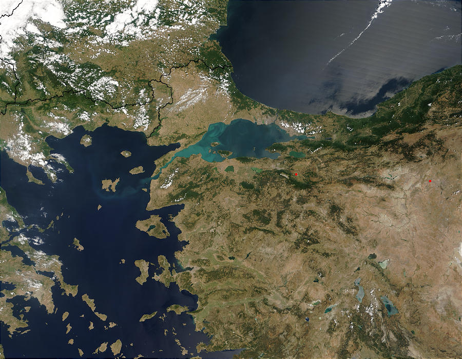
Cite this article
Stanev, E.V., Grashorn, S. & Zhang, Y.J. Cascading ocean basins: numerical simulations of the circulation and interbasin exchange in the Azov-Black-Marmara-Mediterranean Seas system. Ocean Dynamics 67, 1003–1025 (2017). https://doi.org/10.1007/s10236-017-1071-2
Received:
Accepted:
Published:
Issue Date:
DOI: https://doi.org/10.1007/s10236-017-1071-2