
Abstract
An idealized model for tide propagation and amplification in semi-enclosed rectangular basins is presented, accounting for depth differences by a combination of longitudinal and lateral topographic steps. The basin geometry is formed by several adjacent compartments of identical width, each having either a uniform depth or two depths separated by a transverse topographic step. The problem is forced by an incoming Kelvin wave at the open end, while allowing waves to radiate outward. The solution in each compartment is written as the superposition of (semi)-analytical wave solutions in an infinite channel, individually satisfying the depth-averaged linear shallow water equations on the f plane, including bottom friction. A collocation technique is employed to satisfy continuity of elevation and flux across the longitudinal topographic steps between the compartments. The model results show that the tidal wave in shallow parts displays slower propagation, enhanced dissipation and amplified amplitudes. This reveals a resonance mechanism, occurring when the length of the shallow end is roughly an odd multiple of the quarter Kelvin wavelength. Alternatively, for sufficiently wide basins, also Poincaré waves may become resonant. A transverse step implies different wavelengths of the incoming and reflected Kelvin wave, leading to increased amplitudes in shallow regions and a shift of amphidromic points in the direction of the deeper part. Including the shallow parts near the basin’s closed end (thus capturing the Kelvin resonance mechanism) is essential to reproduce semi-diurnal and diurnal tide observations in the Gulf of California, the Adriatic Sea and the Persian Gulf.
1 Introduction
Understanding tidal dynamics is important for coastal safety, navigation, and ecology. The tide in many semi-enclosed basins is the result of co-oscillation with a larger sea, where basin geometry and topography play an important role. Examples of such basins that will be used throughout this study are the Gulf of California, the Adriatic Sea and the Persian Gulf (denoted GoC, Adr, and PGf, respectively). Typical for each of these basins is a relatively shallow zone near the closed end, roughly connected to one (GoC, PGf) or more (Adr) deeper parts, with a symmetric (GoC, Adr) or a clearly asymmetric cross-sectional depth profile (PGf; see Fig. 1). Observations indicate increased amplitudes near the closed end with amplification factors depending on the tidal frequency, which suggests a form of tidal resonance (Garrett 1975; Godin 1993) associated with the topography near the basin’s closed end.

Bathymetric charts of a Gulf of California, b Adriatic Sea, c Persian Gulf. Depth in meters
To reproduce tide observations, numerical models with a detailed representation of geometry and topography have been developed, in some cases using data assimilation to fine-tune the open boundary conditions. This has led to accurate quantitative agreement with tide observations in the Gulf of California (Carbajal and Backhaus 1998; Marinone 2000; Marinone and Lavín 2005), the Adriatic Sea (Malačič et al. 2000; Cushman-Roisin and Naimie 2002; Janeković et al. 2003; Janeković and Kuzmić 2005) and the Persian Gulf (Proctor et al. 1994; Sabbagh-Yazdi et al. 2007). However, a generic model study into the effects of these spatial depth differences on tide propagation and dissipation in semi-enclosed basins, giving insight into the underlying physical mechanisms, is still lacking. This particularly applies to the shallow zone near the closed end of the basins mentioned above and the asymmetric cross-sectional depth profile of the Persian Gulf. In this study, we develop and test such an idealized process-based model, accounting for depth differences by a combination of longitudinal and lateral topographic steps. These topographic steps, seemingly a strong simplification of true bathymetry, are partly motivated by computational considerations explained below, but also by the rather abrupt depth changes seen in real basins. For example, the distinction in a shallow Northern Adriatic, the mid-Adriatic and the deep Southern Adriatic Pit is well recognized (e.g., Artegiani et al. 1997; also see Fig. 1b).
Our idealized process-based model extends the work by Taylor (1922) and several later studies. Taylor (1922) investigated the problem of Kelvin wave reflection in a rotating, rectangular basin of uniform depth. Using the linear depth-averaged shallow water equations on the f plane, the solution can be written as a superposition of analytical wave solutions: an incoming Kelvin wave, a reflected Kelvin wave and an infinite series of Poincaré modes generated at the closed end. A collocation technique can be used to obtain the coefficients of these modes (Brown 1973). Because of rotation, the solution expresses an amphidromic system with elevation amphidromic points (zero tidal range) and current amphidromic points (no velocities), alternatingly found on the centerline of the basin (provided that it is sufficiently narrow such that all Poincaré modes are evanescent). Although Taylor’s solution qualitatively represents the main features of tides in semi-enclosed basins, two strong simplifications are the absence of a dissipation mechanism and the assumption of uniform depth.
Regarding dissipation, Hendershott and Speranza (1971) replaced the no-normal flow condition at the closed end with a partially absorbing one, which reduces the amplitude of the reflected Kelvin wave and shifts the amphidromes away from the centerline. To estimate the absorption coefficients for the Adriatic Sea and the Gulf of California, two generalized Kelvin waves were fitted to tide observations in the central parts of these basins, where the (evanescent) Poincaré waves cannot be felt. Alternatively, Rienecker and Teubner (1980) incorporated a linear bottom friction formulation, which causes damping of the (Kelvin) waves as they propagate, shifting the amphidromes onto a straight line making a small angle with the boundaries. Similar damping and displacement of amphidromes are seen in three-dimensional models, where dissipation is represented using a vertical eddy viscosity and a no-slip (or partial-slip) condition at the bed, see e.g., the Kelvin wave analysis by Mofjeld (1980), the numerical work by Davies and Jones (1995, 1996), and the recent model for elongated basins by Winant (2007). Finally, adding horizontally viscous effects introduces boundary layers and a weak further displacement of the amphidromic points (Roos and Schuttelaars 2009).
Allowing arbitrary depth variations, the eigenmodes can in general no longer be found analytically. Most analytical studies have been restricted to Kelvin waves, e.g., for linear (Hunt and Hamzah 1967; Staniforth et al. 1993), parabolic (Hidaka 1980), and stepwise lateral depth profiles (Hendershott and Speranza 1971), and for linear and exponential longitudinal depth profiles (Godin and Martínez 1994). Note that Hidaka (1980) and Staniforth et al. (1993) also considered Poincaré waves, but in a different way: they fixed the wave number to a real value and solved for the (possibly complex) frequency. This approach is suitable for initial value problems but not for forced problems (Ripa and Zavala-Garay 1999). Instead of using a superposition of eigenmodes, Winant’s (2007) three-dimensional model is based on a truncated power series expansion in the basin’s width-to-length ratio. The solution can be found analytically for a uniform depth and numerically for, e.g., a parabolic lateral profile.
The innovation of our study is twofold. Firstly, we extend Rienecker and Teubner’s (1980) frictional version of Taylor’s (1922) model to account for depth variations in the longitudinal and lateral directions. To this end, we distinguish several adjacent compartments, each having either a uniform depth or two different depths separated by a transverse step. The solution in each compartment can be written as a superposition of wave solutions satisfying the linear shallow water equations, including bottom friction. For a compartment of uniform depth, these solutions are analytically available (Rienecker and Teubner 1980). For a transverse step, they will be derived semi-analytically, following Hendershott and Speranza’s (1971) derivation of Kelvin waves over a sequence of transverse steps, now extending to Poincaré modes and accounting for bottom friction. A collocation technique is then employed to satisfy no-normal flow at the closed end as well as continuity of free surface elevation and water flux across the longitudinal topographic steps between the compartments (matching conditions). Note that Godin (1965) followed a nearly similar approach to model the amphidromic system in Labrador Sea and Baffin Bay (Canada/Greenland), without bottom friction and not aimed at systematically identifying physical mechanisms. To explain ocean-shelf resonance, also Webb (1976) followed this approach, though he neglected bottom friction in the deep (ocean) part and investigated resonance by treating the frequency as a complex quantity.
The second innovation is the way in which we test our idealized model against tide observations in the Gulf of California, the Adriatic Sea and the Persian Gulf. Unlike Hendershott and Speranza’s (1971) study, this comparison covers the full basin, i.e., not only the central part. We compare elevation amplitudes and phases, as they are modeled and observed along the coastline, for four different tidal components: M2, S2, K1 and O1. Our goal is to obtain insight in the dominant physical mechanisms necessary to reproduce the main features of the observed patterns of tide propagation, amplification and dissipation in these basins.
This paper is organized as follows. The model is introduced in Section 2. In Section 3, we present the solution method, including details of the collocation technique (and referring to Appendices A and B for the derivation of wave solutions in channels of uniform depth and channels with a transverse step, respectively). Next, Section 4 contains generic results on the model behavior, identifying two topographic resonance mechanisms. The comparison with tide observations is conducted in Section 5. Finally, Sections 6 and 7 contain the discussion and conclusions, respectively.
2 Model
Consider a tidal wave of angular frequency ω and typical elevation amplitude Z (decimeters to meters), propagating through a rotating, semi-enclosed basin of uniform width B (tens to hundreds of kilometers) and length L (hundreds of kilometers, see Fig. 2). In terms of a horizontal coordinate system with longitudinal coordinate x and lateral coordinate y, the longitudinal basin boundaries are located at y = 0,B, the closed end at x = 0, the open end at x = L. The basin consists of J compartments, separated by longitudinal topographic steps at x = s j . Each compartment either has a uniform depth H = H j (tens to hundreds of meters) or consists of two subcompartments with depths H j and \(H_j^\prime\) (a prime denotes the upper subcompartment; no prime for the lower subcompartment), separated by a transverse step at y = b j (Fig. 2c). Note that the first compartment (j = 1) contains the basin’s closed end, whereas the last compartment (j = J) contains the basin’s open end.

Top view of the model geometry, showing basins of length L, width B and depths H j and \(H_j^\prime\). The three basins used in the comparison are sketched: a Gulf of California (one step, H1 < H2), b Adriatic Sea (two steps, H1 < H2 < H3), c Persian Gulf (combination of longitudinal and transverse step, \(H_1=H_2<H_2^\prime\)). The solution along the basin perimeter PQRS will be used in the comparison with observations; the lines Q′R′ and Q′′R′′ represent the longitudinal steps at x = s1 and x = s2, respectively
Assuming that the surface elevation amplitude is much smaller than the water depth, conservation of mass and momentum is expressed by the linear depth-averaged shallow water equations on the f plane, including bottom friction:
Here, ζ j denotes the free surface elevation (with respect to still water z = 0); u j and \(\emph{v}_j\) are the depth-averaged flow velocity components in x and y-direction, respectively, and t is time. The scaling procedure justifying Eqs. 1–3 is not presented here, see e.g., Roos and Schuttelaars (2009). We merely state the implications: nonlinear advection terms are absent and the mean water depth H j (rather than the true water depth H j + ζ j ) appears in the denominator of the friction terms and in the continuity equation. In the case of a transverse step, the solution in the upper subcompartment is denoted with a prime; we then solve Eqs. 1–3 for the primed variables \((\zeta_j^\prime,u_j^\prime,\emph{v}_j^\prime)\) and primed parameters \((r_j^\prime,H_j^\prime)\). Variables and parameters without primes are used to denote the solution in the lower subcompartment.
In Eqs. 1–2, f = 2Ωsinϑ is a Coriolis parameter, with Ω = 7.292×10 − 5 s − 1 the angular frequency of the Earth’s rotation and ϑ the latitude. Moreover, g = 9.81 m s − 2 is the acceleration of gravity. We have introduced a linear bottom friction term with coefficient
obtained from Lorentz’ linearization of a quadratic friction law (Zimmerman 1982) with a default value of the drag coefficient C D and typical flow velocity scale U j . Since the water depth is likely to influence U j , we allow each (sub)compartment to have a different bottom friction coefficient r j (or \(r_j^\prime\)). Calculating each friction coefficient thus requires an estimate of the flow velocity scale, which we define as the square root of the (squared) velocity amplitude averaged over the (sub)compartment. The friction coefficients are obtained using an iterative procedure, explained in Section 3.3. An advantage of this procedure is that only one friction parameter, i.e., the drag coefficient C D, must be specified, while accounting for the local feedback of higher (lower) flow velocities onto larger (smaller) values of the friction coefficient.
No-normal flow across the closed boundaries implies
thus accounting for the upper and lower boundaries of each compartment (j = 1, ⋯ ,J) as well as the basin’s closed end in the first compartment, respectively. Across topographic steps, we require continuity of surface elevation and water flux (matching conditions). For a longitudinal step, this gives
where a subscript denotes the solution in the corresponding compartment (j = 1, ⋯ ,J − 1). For a transverse step, the matching conditions read
where a prime denotes the solution in the upper subcompartment (no prime for the lower subcompartment). Note that the quantities in Eqs. 7 and 8, due to the discontinuity in depth, need not be differentiable across the topographic steps. Finally, the problem is forced by an incoming Kelvin wave at x = L, while allowing reflected Kelvin and (free) Poincaré waves to radiate outward. In fact, this is equivalent to letting the last compartment stretch to infinity, and imposing an incoming Kelvin wave from infinity as the forcing of our problem.
3 Solution method
3.1 Superposition of wave solutions
Let \(\phi_j=(\zeta_j,u_j,\emph{v}_j)\) symbolically represent the system’s state in compartment j. We seek time-periodic solutions of the form
where \(\Re\) denotes the real part and ω is the angular frequency. For compartment j, the vector \(\hat{\phi}_j=(\hat{\zeta}_j,\hat{u}_j,\hat{\emph{v}}_j)\) contains the complex amplitudes of surface elevation, longitudinal and lateral flow velocity, respectively.
The key step is now to write the solution in each compartment as a truncated sum of (semi)-analytical wave solutions in an infinite channel. This involves Kelvin modes propagating in the positive and negative x-direction, as well as Poincaré modes, generated at the closed end and on either side of each topographic step. For all compartments (except the last one, so j = 1,...,J − 1), we thus write
with truncation number M (and defining s 0 = 0). Here, \(\tilde{\phi}_{j,m}^\oplus(y)\) and \(k_{j,m}^\oplus\) are the lateral structure and the wave number, respectively, corresponding to the mth mode propagating (if free) or exponentially decaying (if evanescent) in the positive x-direction. This involves both Kelvin modes (m = 0) and Poincaré modes (m = 1,2,...,M), which are generated (i.e., reflected or transmitted) at the interface x = s j − 1 on the left. The opposite modes, i.e., propagating or decaying in the negative x-direction and denoted with a superscript ⊝ , are generated at the interface x = s j on the right. To make sure that the coefficients \(a_{j,m}^\oplus\) and \(a_{j,m}^\ominus\) are of the same order as Z, the exponential functions in Eq. 10 have been normalized to unity at the interfaces x = s j − 1 and x = s j , respectively.
Due to the open boundary at x = L, the last compartment J requires a different form of the solution. Since we neglect the Poincaré modes bound to the open end (x = L), the only mode propagating or decaying in the negative x-direction is the incoming Kelvin wave, with coastal amplitude Z and initial phase φ (both at x = L). This gives
The wave solutions in an infinite channel of uniform depth (Rienecker and Teubner 1980), along with their symmetry properties, are given in Appendix A. Wave solutions in an infinite channel with a transverse step are derived in Appendix B.
3.2 Collocation technique
Since each of the individual wave solutions in Eqs. 10 and 11 satisfies the no-normal flow condition at the closed boundaries y = 0 and y = B according to Eq. 5, so do the superpositions \(\hat{\phi}_j\) and \(\hat{\phi}_J\). A collocation technique is used to satisfy the no-normal flow condition at the closed end in Eq. 6 and the matching conditions Eq. 7, as well (Fig. 3).

Collocation points used to satisfy no-normal flow at the basin’s closed end (open circles) and continuity of elevation ζ and flux Hu across the topographic steps (solid circles). Combined sets of Kelvin/Poincaré modes are indicated by double arrows, pointing in the direction of propagation/decay; a single arrow represents the incoming Kelvin wave. Examples as in Fig. 2, truncation number M = 8
Defining M + 1 lateral points y n = Bn/M for n = 0,1,...,M, we require
for n = 0,1,...,M and j = 0,...,J − 1. This leads to a linear system of equations for the (2J + 1) (M + 1) coefficients \(a_{j,m}^\oplus\) and \(a_{j,m}^\ominus\), which is solved using standard techniques.
3.3 Iterative procedure to calculate friction coefficient
Calculating the bottom friction coefficient r j (or \(r_j^\prime\)) in each (sub)compartment using Eq. 4 requires a typical velocity scale U j (or U j ′). This quantity is defined as the square root of the squared velocity amplitude, averaged over compartment j, i.e.
or, in the case of a transverse step,
To proceed, we adopt an iterative procedure. At first guess, r j is obtained from Eq. 4 using the typical velocity scale of a classical Kelvin wave without friction: \(U_j=Z\sqrt{g/H_j}\) (Pedlosky 1982). Next, evaluation of the solution leads to new U j -values and thus to new r j -values, which in turn lead to a new solution, and so forth. The same applies to \(r_j^\prime\) and \(U_j^\prime\) in the case of a transverse step. As it turns out, this method converges rapidly. Note that the feedback of the solution on the values of the friction coefficients is in fact a nonlinear element in an otherwise linear model.
4 Results
4.1 Qualitative properties
To investigate the model results qualitatively, let us consider the semi-diurnal lunar tide (“M2”) in a sample basin, at a latitude of 45°N with a width B = 200 km, a length L = 600 km and a reference depth of 50 m. We now distinguish four different topographies: (a) the reference case of uniform depth, (b) a shallow zone of 20 m depth near the basin’s closed end bounded by a longitudinal step at x = 200 km, (c) a transverse step at y = 100 km, with a shallow lower subcompartment of 20 m depth (type I), (d) a transverse step at y = 100 km with a shallow upper subcompartment of 20 m depth (type II).
Figure 4 displays the amphidromic systems of these four cases, showing the results both without (top row, Fig. 4a–d) and with bottom friction (bottom row, Fig. 4e–h). The shallow zones are indicated with a grey shade. In the simulations, the coastal elevation amplitude of the incoming Kelvin wave at x = L is Z = 1 m, and we used truncation numbers M = 16 (and M = 15 in the case of a transverse step; an odd number to avoid a collocation point positioned exactly at the transverse step). Note that, for both the shallow and deep part, the channel width is below the critical channel width such that all Poincaré mode are evanescent.

Amphidromic system of the M2-tide in the sample basin, without (top row, i.e., a–d) and with friction (bottom row, i.e., e–h), shallow zones shaded in grey. From left to right: a and e uniform depth, b and f shallow end, c and g transverse step of type I (shallow lower subcompartment), d and h transverse step of type II (shallow upper subcompartment). Co-phase lines (in red) spiral outward from amphidromic points (tidal period in 12 intervals), co-range contours in red; contour interval equals 20 cm and the basin’s closed end is on the left (at x = 0). For parameter values, see text
The reference case in Fig. 4a is the classical Taylor solution, with elevation and current amphidromic points alternatingly on the centerline of the basin. In this case, the Kelvin wavelength equals 990 km. Including a shallow end (Fig. 4b) leads to amplified amplitudes and flow velocities in the shallow end. Furthermore, the amphidromic points shift towards the closed end, which is due to the smaller tidal wavelength in the shallow part (626 km). The Taylor solution with a transverse step generally shows a shift of amphidromic points toward the deeper part. In Fig. 4c, the incoming Kelvin wave is bound to the coastline of the deep part, the reflected Kelvin wave to the coastline of the shallow part (Northern Hemisphere). By conservation of wave power, the associated decrease in wavelength of the turning tidal wave (from 904 to 714 km) leads to increased elevation amplitudes in the shallow subcompartment. Compared to the uniform depth case, this pushes the amphidromes away from the centerline, into the (deeper) upper subcompartment. The situation in Fig. 4d is opposite; the turning Kelvin wave now experiences an increase in wavelength (from 714 to 904 km). This lowers the amplitude of the reflected Kelvin wave, which pushes the amphidromes away from the centerline into the (deeper) lower subcompartment. Note that the Kelvin wavelengths obtained here for a channel with a transverse step are in between the wavelengths in a channel of the same depths but then distributed uniformly (626 and 990 km; see above).
The main effect of including friction is the exponentially decaying Kelvin wave amplitude in the direction of propagation (Rienecker and Teubner 1980; Roos and Schuttelaars 2009). Regardless the chosen topography, amphidromic points thus shift toward the coast to which the reflected Kelvin wave is bound (Fig. 4e–h). Sufficiently far away from the closed end, this may lead to so-called virtual amphidromic points, located outside the basin. The shift in amphidromes toward the lower coast can be seen for the reference case with friction, by comparing Fig. 4a with e. Adding friction to the case with a shallow end leads to a stronger decay of the reflected Kelvin wave as it propagates and turns in the shallow part, and thus to a stronger shift of the amphidromic points towards the lower coastline (Fig. 4f). This shift is also seen from the two cases with a transverse topographic step (Fig. 4g, h). Hence, depending on the type of transverse step, frictional effects either counteract the inviscid displacement of amphidromic points (type I) or amplify it (type II).
Changing the parameter values of our sample basin will affect the quantitative properties, but not the qualitative picture.
4.2 Kelvin and Poincaré resonance
Now let us further analyze the tidal amplification, associated with the presence of a shallow zone near the basin’s closed end (Figs. 2a, 4b and 4f). To this end, we define the amplification factor A as the ratio of the elevation amplitude, averaged across the closed end (line QR in Fig. 2a), and the coastal elevation amplitude of the incoming Kelvin wave at the topographic step (x = s 1, point Q ′). Below we will identify two topographic resonance mechanisms, associated with amplification of either Kelvin modes or Poincaré modes.
The first resonance mechanism exists also in the absence of rotation (f = 0). The problem with a single topographic step is then nearly similar to that described by (Godin 1993). As shown in Appendix C, the solution can be found analytically. In the case without bottom friction, the amplification rate is found to be
with \(K_1=\omega/\sqrt{gH_1}\). Hence, assuming H 2 > H 1, maximum amplification (resonance) occurs if cosK 1 L 1 = 0, i.e., if the length of the shallow end is an odd multiple of a quarter of the frictionless Kelvin wavelength λ 1,0 = 2π/K 1 in the shallow part:
The corresponding amplification rate is proportional to the square root of the ratio of water depths: \(A_\mathrm{1D,max}=2\sqrt{H_2/H_1}\). Conversely, minimum amplification occurs if cosK 1 L 1 = 1, giving A 1D,min = 2. This factor 2 is due to the standing wave character: the elevation amplitude at the closed end is twice the amplitude of the incoming wave.
To investigate the amplification for the case with rotation (\(f\ne0\)), we will now vary the dimensions of the shallow compartment (length L 1, basin width B), while taking the other parameter values from the Gulf of California case (Table 1). Figure 5 shows the scaled amplification rate A/A 1D,max of four tidal constituents (M2, S2, K1, and O1) as obtained with our model, relative to the one-dimensional maximum without bottom friction introduced above. The figure shows the results without (top row) and with bottom friction (bottom row), where L 1 and B have both been scaled against the frictionless Kelvin wavelength λ 1,0 = 2π/K 1 in the shallow part.

Amplification factor A/A 1D,max, as a function of the dimensions of the shallow compartment, without (top row, i.e., a–d) and with bottom friction (bottom row, i.e., e–h). This has been done for four tidal components: a and e M2, b and f S2, c and g K1, d and h O1. Parameter values taken from the Gulf of California (Table 1), the actual dimensions of the Gulf of California’s shallow part in each plot being denoted with a circle. The case denoted with a rectangle in (a) is shown in Fig. 6d. The A/A 1D,max = 1-contour is plotted as a black line in (a) and (b)
As can be seen from the curved contours in Fig. 5, rotation introduces a width-dependency to the amplification rate, whereas the Kelvin resonance mechanism explained above can still be identified. As an example of Kelvin resonance, Fig. 6c presents the amphidromic system of the GoC-case without bottom friction (dimensions corresponding to the circle in Fig. 5a). In the limit B ↓ 0, we recover the analytical amplification rates without rotation, i.e., Eq. 18 without friction and Eq. 45 in Appendix B with friction. The dependency on width is more apparent for wide basins and for stronger rotation (larger f/ω-values). In particular, for \(B\approx \frac{1}{2}\lambda_{1,0}\) in Fig. 5a, b, we obtain amplification rates exceeding the one-dimensional maximum A 1D,max mentioned above.

Amplification in the (L 1,B)-plane, as obtained from a the theoretical resonance curves according to Eqs. 19 and 20, and b the model results, i.e. the amplification factor A/A 1D,max for weak rotation (f/ω = 0.09, corresponding to e.g., an M2-tide at a latitude ϑ = 5°N). Ratio of water depths H 2/H 1 = 12, no friction. c and d provide examples of Kelvin and Poincaré resonance, corresponding to the circle and square in Fig. 5a, respectively
A second resonance mechanism underlies these amplification rates, associated with a Poincaré mode that is free in the shallow part yet evanescent in the deep part. As an example of Poincaré resonance, Fig. 6d shows the amphidromic system corresponding to the square in Fig. 5a, which resembles a transverse sloshing mode. Understanding this type of amplification in our Kelvin-wave-forced problem is less straightforward than the Kelvin resonance described above; it can best be understood by considering the case of weak rotation (f/ω ≪ 1). According to Eqs. 27 and 28 in Appendix A, the transverse structure of the elevation and longitudinal flow of the mth Poincaré mode is then dominated by the part proportional to cosα m y (with α m = mπ/B). Now let us consider a balance between a standing mth Poincaré mode in the shallow part (i.e., a superposition of two Poincaré modes that satisfies no normal flow at the closed end according to Eq. 12) and the mth Poincaré mode in the deep part. Requiring their contributions proportional to cosα m y to satisfy the matching conditions in Eq. 7 leads to a relationship between L 1 and B:
Here, k 1,m and k 2,m are the wave numbers of the mth Poincaré mode in the shallow and deep compartment, respectively, according to Eq. 26 in Appendix A. As shown in Fig. 6a, b, the agreement between these theoretical resonance curves and the model results is excellent (for f/ω small). Increasing the value of f/ω, still excluding bottom friction, leads to a more smoothed amplification pattern with lower resonance peaks (see top row of Fig. 5).
Comparison between the top row and bottom row in Fig. 5 shows that including bottom friction leads to a further overall damping of the amplification rate, also smoothing the amplification rates associated with the two resonance mechanisms explained above. Finally, the circles in Fig. 5e–h show that the shallow part in the Gulf of California experiences maximum amplification for the semi-diurnal tides (M2 and S2), whereas it is clearly further away from resonance for the diurnal tides (K1 and O1).
5 Comparison with observations
5.1 Method
In this section, we will test our idealized model by comparing with tide observations in the Gulf of California, the Adriatic Sea and the Persian Gulf. The comparison will be carried out for the coastal amplitudes and phases of four predominant tidal components: M2, S2 (semi-diurnal), K1, and O1 (diurnal). The combined pattern of elevation amplitudes and phases, observed at the tide stations along the coastline, provides a clear footprint of the tidal dynamics in the entire basin. Our procedure consists of the following four steps.
-
1.
Find, on the f plane around the basin’s center (latitude ϑ), the rectangular model basin geometry PQRS that provides a best fit of the coastline (Fig. 7). To this end, we choose the basin’s position, width B and orientation such that the average distance from the available tide stations to the basin boundaries is minimized.
Fig. 7 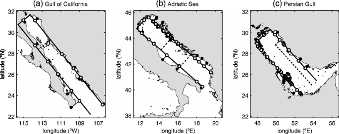
Coastlines and model geometries of the basins used in the comparison: a Gulf of California, b Adriatic Sea, and c Persian Gulf. Also shown are the tide stations (solid circles), their projections onto the model basin boundary (open circles) and the topographic steps (dashed lines)
-
2.
Perform an orthogonal projection of each tide station onto the basin boundaries. This allows us to consider the observed elevation amplitudes and phases as a function of a single coordinate: the distance along the perimeter PQRS. The longitudinal distance from corner point to the farthest (projected) tide station defines the basin length L.
-
3.
Based on bathymetric charts, roughly choose the remaining geometrical parameters, i.e., the number of compartments as well as their lengths L j and depths H j . In the case of a compartment with a transverse step (PGf), this also involves specifying the location y = b j of the transverse step as well as the two depths H j and \(H_j^\prime\) of the lower and upper subcompartment, respectively.
-
4.
Make simulations by varying the amplitude Z (and phase φ) of the incoming Kelvin wave. Herein, the Coriolis parameter f is based on the basin’s central latitude ϑ, the friction coefficients r j are calculated iteratively as explained in Section 3.3.

The parameter settings and other information relevant to the model validation are shown in Table 1. The Kelvin wavelength and e-folding decay distance of the first Poincaré mode are given by
respectively (where \(\Re\) denotes the real part and \(\Im\) the imaginary part). In the case of a transverse step, the symbols ⊕ and ⊝ are used to distinguish the modes propagating or decaying in the positive x-direction from those propagating or decaying in the negative x-direction. Furthermore, the dimensionless friction coefficient r j /(ωH j ) quantifies the relative importance of bottom friction with respect to inertia.
The observed amplitudes and phases are taken from several sources: Carbajal and Backhaus (1998) for the Gulf of California, Janeković et al. (2003) and Janeković and Kuzmić (2005) for the Adriatic Sea, and British Admiralty (2009) for the Persian Gulf.
5.2 Gulf of California
The Gulf of California has mixed semi-diurnal tides and one of the largest tidal ranges on Earth, particularly in the northern region. The geometry with a shallow Northern Gulf and a deeper Southern Gulf is represented using two compartments of depths 100 m and 1,200 m (Fig. 7a), the topographic step located near the two large islands. To guarantee a proper basin shape in the Gulf of California, where only 11 tide stations are available, we included the coordinates of nine other coastal locations.
The results are plotted in Fig. 8, showing good agreement regarding both amplitude and phase. The phase curves in Fig. 8e, f contains a maximum, which is indicative of a virtual amphidromic point, which in turn is due to strong friction. Note that the diurnal components are much weaker than the semi-diurnal ones, hardly showing any phase variations.

Comparison of model results (solid line) and observations (circles) for four tidal components in the Gulf of California: M2, S2, K1, and O1. The plots show amplitudes (top) and phases (bottom), both as a function of the perimeter coordinate along PQRS. The points Q ′ and R ′ indicate the transitions from deep to shallow and vice versa, respectively
5.3 Adriatic Sea
Unlike the rest of the Mediterranean Sea, where tides are weak, the Adriatic Sea has moderate tides of the mixed type. The bathymetry of the Adriatic Sea shows three rather distinct compartments (Fig. 7b): the relatively shallow Northern Adriatic (north of the 100 m-isobath), the mid-Adriatic Pit and the Southern Adriatic Pit (with depths exceeding 1,000 m). In our comparison, we have neglected the tide stations located on islands in the basin’s interior (Vis, Komiza, Svetac and Palagruza).
As shown in Fig. 9, we obtain good agreement, except for the amplitudes at the tide stations in the northeast of the Adriatic (near point Q). The semi-diurnal phase curves in Fig. 9e, f show a continuous increase along the basin perimeter, which is indicative of an amphidromic point inside the basin, in turn showing that dissipation is weak. Like in the Gulf of California, the phase variations of the diurnal components are much weaker than the semi-diurnal ones. Malačič et al. (2000) stated that the diurnal tides in the Adriatic Sea cannot be explained by Taylor’s approach, but rather as topographic waves propagating across the basin. However, our extension of Taylor’s model, by adding longitudinal topographic steps, gives good agreement also for diurnal tides.

Same as Fig. 8, but now for the Adriatic Sea. The points Q ′ ′ and R ′ ′ mark the transition from deep to shallow and vice versa at the second topographic step
5.4 Persian Gulf
The tidal pattern in the Persian Gulf varies from being primarily semi-diurnal to diurnal (Proctor et al. 1994). Semi-diurnal constituents have two amphidromic points in the north-western and southern ends of the Gulf; diurnal constituents have a single amphidromic point in the center. Hydrodynamic simulations predict tidal flows exceeding 0.5 m s − 1.
The topography of the Persian Gulf is modeled as in Fig. 7c, i.e., by a combination of the configurations discussed in Section 4 (Fig. 4b, c). The shallow zone near the closed end extends all the way along the southern part of the basin, leading to a strongly asymmetrical cross-sectional depth profile of the main part. The depth difference between the shallow (30 m) and the deeper part (50 m) is less pronounced than in the other basins under consideration.
The results are plotted in Fig. 10, generally showing good agreement regarding amplitude and phase. Two large-scale complications of the coastline are Qatar Peninsula (giving some scatter when plotting tide observations in Fig. 10) and the coastline near the United Arab Emirates and the Strait of Hormuz (tide stations not included). We have furthermore excluded the tide stations located far into the basin’s interior, i.e., on islands or oil rigs, and those located at upstream locations in rivers or estuaries.

Same as Fig. 8, but now for the Persian Gulf
6 Discussion
6.1 Model approach and method
The model approach is computationally efficient (allowing us to make large numbers of simulations as required in e.g., Figs. 5 and 6) and can in principle be applied to any semi-enclosed basin with roughly a rectangular basin shape. We have elaborated the case of a single transverse step, which is suitable for the central part of the Persian Gulf. The extension towards two or more transverse steps is straightforward: wave solutions can be found in a way analogous to Appendix B. In the collocation method, one should avoid collocation points exactly at the position of a transverse step, because the longitudinal velocity is not uniquely defined.
Within our approach of compartments separated by longitudinal depth steps, it is perhaps tempting to allow for steps in basin width, as well (Godin 1965). However, this introduces reflex angles in the coastline where the solution may not be smooth. This is likely to be a manifestation of Gibbs’ phenomenon.
Our open boundary condition (an incoming Kelvin wave, while allowing other waves to radiate outward) neglects the precise geometry and flow properties near the basin’s open end PS, where it connects to the outer sea (Mediterranean, Pacific, Strait of Hormuz/Gulf of Oman). The role of Poincaré modes, generated near the open end, is therefore neglected, as well. The influence of these modes is restricted to a few Poincaré decay lengths from the line PS, roughly 50–100 km (Table 1). In that region, it is therefore not meaningful to strictly compare our model results with observations. However, the solution in the other parts is not affected by the open end.
We realize that there is some freedom in the choice of basin geometry for the comparison with observations. In the spirit of our idealized approach, the number of (sub)compartments is minimized, while accounting for the major topographic elements in the basins under consideration. Including more detail by adding more compartments is likely to improve the agreement with observations, but we did not undertake this exercise as it does not add to our understanding. Next, the results turn out not to be very sensitive to the choice of depth and the positions of the topographic steps, which we based on bathymetric charts (e.g., see Fig. 1). An indication of the sensitivity to the various geometric parameters can be found in Fig. 5.
The procedure according to which we fit the basin geometry is affected by the number and distribution of the available tide stations. As it turns out, tidal phases are reproduced more accurately than the amplitudes. Apparently, the phase suffers relatively little from the schematizations in the idealized model and projection procedure. The amplitudes are more sensitive to irregularities in coastline, the presence of islands and local depth variations.
6.2 Topographic steps and wave dynamics
The presence of longitudinal and transverse topographic steps introduces new elements to the wave dynamics. First of all, depth affects the properties of the fundamental wave solutions in the compartments with a uniform depth (Appendix A). This includes the properties of the Kelvin mode (wavelength, dissipation, Rossby deformation radius and other aspects of the transverse structure) and Poincaré modes (e-folding decay distance or wavelength, dissipation, transverse structure).
The interface conditions to be satisfied at the longitudinal topographic steps also introduces new aspects to the wave dynamics. For example, Hendershott and Speranza (1971) use the term “edge waves” to denote waves that may ‘travel across the zone of rapid shoaling towards the end of the bay’, i.e., along the longitudinal topographic step. The possibility for such wave behavior is contained in our model; it is expressed by the Poincaré waves generated on either side of the step. The Poincaré resonance mechanism identified in our study is in fact an extreme manifestation of this phenomenon. In the next subsection, the relevance of Kelvin and Poincaré resonance will be discussed.
Our analysis has furthermore shown that, in compartments with a transverse step, Kelvin and Poincaré modes continue to exist (Appendix B), with the transverse step modifying their properties. The most striking example is perhaps the difference in wavelength of the incoming and reflected Kelvin wave (Section 4). In addition, one may expect to encounter a wave solution acting as the channel-type counterpart of a so-called double Kelvin wave. These waves, as shown by Longuet-Higgins’s (1968) analysis for an unbounded sea, may propagate along discontinuities in depth. The periods associated with double Kelvin waves, however, are well above those of the semi-diurnal and diurnal tides investigated in our study, particularly for relatively small depth ratios (\(H_2^\prime/H_2<2\) for PGf; cf. Fig. 3 in Longuet-Higgins 1968). This explains why such modes are not encountered in our analysis.
6.3 Relevance of topographic resonance mechanisms
The model results for the Gulf of California clearly express the combined effect of topographically induced (Kelvin) resonance and bottom friction (whereas Hendershott and Speranza (1971) mention only the latter). Inclusion of the shallow zone is necessary to obtain the amplified amplitudes near the basin’s head. In turn, only these amplified amplitudes over the shallow zone are capable of inducing the dissipation required to obtain a virtual amphidromic point (at the correct position). These considerations are supported by simulations for a uniform depth (graphs not reported here), carried out for different depths and amplitudes, which fail to reproduce the amphidromic system of the Gulf of California. These simulations either show too little dissipation and hence a real amphidrome or require unrealistically large elevation amplitudes for a virtual amphidrome to occur. For the Adriatic Sea, where dissipation is almost negligible, simulations with a uniform depth fail to reproduce the observed amplification near the basin’s head, and miss important details of the observed amplitude and phase curve (associated with errors in local wave speed). In their comparison between the semi-diurnal tides in the Gulf of California and the Adriatic sea, Hendershott and Speranza (1971) discuss the importance of bottom friction without mentioning the topographically induced amplification.
Poincaré resonance, the second mechanism identified in Section 4.2, is less likely to be observed in semi-enclosed basins in reality. This is because it requires rather large basin widths, for semi-diurnal and diurnal tides. For higher harmonics (e.g., M4, M6), these critical widths are smaller. Note that the Poincaré resonance mechanism identified in our study, triggered by an incoming Kelvin wave and involving a Poincaré mode that is free in the shallow part yet evanescent in the deep part, differs from that analyzed by Buchwald (1980) in the context of ocean-shelf resonance. He described the quarter-wavelength resonance of an incident, free wave without any lateral structure in a domain with a longitudinal topographic step but without lateral boundaries.
7 Conclusion
We have extended Rienecker and Teubner’s (1980) frictional version of Taylor’s (1922) classical model of Kelvin wave reflection in a semi-enclosed, rectangular, rotating basin of uniform depth to account for the presence of longitudinal and lateral topographic steps. In doing so, the model’s idealized nature has been retained, allowing the solution in the various compartments to be written as a superposition of wave solutions. These wave solutions are available analytically from earlier studies in the case of a compartment with a uniform depth (Rienecker and Teubner 1980); they have now been derived semi-analytically in the case of a transverse step. A collocation method is used to satisfy no-normal flow across the basin’s closed end and continuity of surface elevation and longitudinal flux across the longitudinal topographic steps.
The model results indicate slower tide propagation, enhanced dissipation and the possibility of amplified amplitudes in the shallow part. In particular, two resonance mechanism have been identified. Kelvin resonance occurs when the length of the shallow end is roughly an odd multiple of a quarter Kelvin wavelength. Alternatively, also Poincaré waves may become resonant, but this requires rather wide basins. A transverse step mainly causes the incoming and reflected Kelvin wave to have different wavelengths. Conservation of wave power then leads to increased amplitudes in shallow regions and a shift of amphidromic points in the direction of the deeper part.
We compared our idealized model results with tide observations (coastal elevation amplitudes and phases) in the Gulf of California, the Adriatic Sea and the Persian Gulf. Despite the strong simplifications regarding geometry (rectangular basin) and topography (combination of longitudinal and lateral topographic steps), we obtain good agreement for both the semi-diurnal and diurnal constituents. We conclude that capturing the Kelvin resonance mechanism is essential herein.
Finally, our idealized model can be used as a quick tool to assess the impact (order of magnitude, area of influence) of human intervention before performing simulations using detailed numerical models with a more realistic geometry. Examples of human intervention that may affect tidal dynamics in semi-enclosed basins are various long-term future scenarios of (extremely) large-scale dredging operations and land reclamation.
References
Artegiani A, Bregant D, Paschini E, Pinardi N, Raicich F, Russo A (1997) The Adriatic Sea general circulation. Part I: air-sea interactions and water mass structure. J Phys Oceanogr 27(8):1492–1514
British Admiralty (2009) NP203-2010 Admiralty Tide Tables 2010, vol 3. United Kingdom Hydrographic Office
Brown PJ (1973) Kelvin-wave reflection in a semi-infinite canal. J Mar Res 31(1):1–10
Buchwald VT (1980) Resonance of Poincaré waves on a continental shelf. Aust J Mar Fresh Res 31(4):451–457. doi:10.1071/MF9800451
Carbajal N, Backhaus JO (1998) Simulation of tides, residual flow and energy budget in the Gulf of California. Oceanol Acta 21(3):429–446
Cushman-Roisin B, Naimie CE (2002) A 3D finite-element model of the Adriatic tides. J Mar Syst 37(4):279–297. doi:10.1016/S0924-7963(02)00204-X
Davies AM, Jones JE (1995) The influence of bottom and internal friction upon tidal currents: Taylor’s problem in three dimensions. Cont Shelf Res 15(10):1251–1285
Davies AM, Jones JE (1996) The influence of wind and wind wave turbulence upon tidal currents: Taylor’s problem in three dimensions with wind forcing. Cont Shelf Res 16(1):25–99
Garrett C (1975) Tides in gulfs. Deep-Sea Res 22(1):23–35
Godin G (1965) The M2 tide in the Labrador Sea, Davis Strait and Baffin Bay. Deep Sea Res 12(4):469–477
Godin G (1993) On tidal resonance. Cont Shelf Res 13(1): 89–107
Godin G, Martínez A (1994) On the possibility of Kelvin-type motion in actual seas. Cont Shelf Res 14(7-8):707–721
Hendershott MC, Speranza A (1971) Co-oscillating tides in long, narrow bays; the Taylor problem revisited. Deep-Sea Res 18(10):959–980
Hidaka K (1980) Poincaré waves and Kelvin waves in a straight canal of parabolic section. Proc Japan Acad B 56(6):312–316
Hunt JN, Hamzah AMO (1967) Tidal waves in a canal of non-uniform depth. Pure Appl Geophys 67(1):133–141. doi:10.1007/BF00880571
Janeković I, Kuzmić M (2005) Numerical simulation of the Adriatic Sea principal tidal constituents. Ann Geophys 23(10):3207–3218
Janeković I, Kuzmić M, Bobanović J (2003) The Adriatic Sea M2 and K1 tides by 3D model and data assimilation. Est Coast Shelf Sci 57(5-6):873–885. doi:10.1016/S0272-7714(02)00417-1
Longuet-Higgins MS (1968) On the trapping of waves along a discontinuity of depth in a rotating ocean. J Fluid Mech 31(3):417–434
Malačič V, Viezzoli D, Cushman-Roisin B (2000) Tidal dynamics in the northern Adriatic Sea. J Geophys Res 105(C11):26,265–28,280
Marinone SG (2000) Tidal currents in the Gulf of California: Intercomparisons among two- and three-dimensional models with observations. Ciencias Marinas 26(2):275–301
Marinone SG, Lavín MF (2005) Tidal current ellipses in a three-dimensional baroclinic numerical model of the Gulf of California. Est Coast Shelf Sci 64(2-3):519–530. doi:10.1016/j.ecss.2005.03.009
Mofjeld HO (1980) Effects of vertical viscosity on Kelvin waves. J Phys Oceanogr 10(7):1039–1050
Pedlosky J (1982) Geophysical Fluid Dynamics. Springer-Verlag
Proctor R, Flather RA, Elliott AJ (1994) Modelling tides and surface drift in the Arabian Gulf— application to the Gulf oil spill. Cont Shelf Res 14(5):531–545
Rienecker MM, Teubner MD (1980) A note on frictional effects in Taylor’s problem. J Mar Res 38(2):183–191
Ripa P, Zavala-Garay J (1999) Ocean channel modes. J Geophys Res 104(C7):15,479–15,494
Roos PC, Schuttelaars HM (2009) Horizontally viscous effects in a tidal basin: extending Taylor’s problem. J Fluid Mech 640:423–441. doi:10.1017/S0022112009991327
Sabbagh-Yazdi SE, Zounemat-Kermani M, Kermani A (2007) Solution of depth-averaged tidal currents in Persian Gulf on unstructured overlapping finite volumes. Int J Numer Meth Fluids 55(1):81–101. doi:10.1002/fld.1441
Staniforth AN, Williams RT, Neta B (1993) Influence of linear depth variation on Poincaré, Kelvin and Rossby waves. J Atmos Sci 50(7):929–940
Taylor GI (1922) Tidal oscillations in gulfs and rectangular basins. Proc Lond Math Soc 20(1):148–181. doi:10.1112/plms/s2-20.1.148
Webb DJ (1976) A model of continental-shelf resonances. Deep Sea Res 23(1):1–15
Winant CD (2007) Three-dimensional tidal flow in an elongated, rotating basin. J Phys Oceanogr 37(9):2345–2362. doi:10.1175/JPO3122.1
Zimmerman JTF (1982) On the Lorentz linearization of a quadratically damped forced oscillator. Phys Lett A 89(3):123–124
Acknowledgements
This work is supported by the Netherlands Technology Foundation STW, the applied science division of NWO, and the Netherlands Ministry of Economic Affairs. The authors thank two anonymous reviewers for their comments.
Open Access
This article is distributed under the terms of the Creative Commons Attribution Noncommercial License which permits any noncommercial use, distribution, and reproduction in any medium, provided the original author(s) and source are credited.
Author information
Authors and Affiliations
Corresponding author
Additional information
Responsible Editor: Roger Proctor
Appendix
Appendix
1.1 A Wave solutions in a channel of uniform depth
This appendix contains analytical expressions of the wave solutions in an infinitely long channel of uniform width B and uniform depth H j (with j = 1,2), including bottom friction:
with amplitude factor Z ′ (in m), wave number \(k_{j,m}^\oplus\) and lateral structures \(\tilde{\zeta}_{j,m}^\oplus(y)\), \(\tilde{u}_{j,m}^\oplus(y)\) and \(\tilde{\emph{v}}_{j,m}^\oplus(y)\). For the Kelvin mode (m = 0) propagating in the positive x-direction, we obtain
respectively. Here, we have used the reference wave number K j , the Rossby deformation radius R j (both typical for a classical Kelvin wave without friction) and a frictional correction factor, given by
respectively.
The wave number and lateral structures of the mth Poincaré mode (m > 0) propagating (if free) or decaying (if evanescent) in the positive x-direction are given by
respectively, with α m = mπ/B.
The modes propagating or decaying in the negative x-direction are defined analogous to Eq. 22, but now using a superscript ⊝ instead of a superscript ⊕ . By symmetry, the two type of modes \(\tilde{\phi}_{j,m}^\oplus\) and \(\tilde{\phi}_{j,m}^\ominus\) satisfy the following relationships:
This symmetry does not hold in the case of a transverse step, which is elaborated in Appendix B.
1.2 B Wave solutions in a channel with a transverse step
Wave solutions in an infinite channel with a transverse step at \(y=b_{j}\) consist of a solution in the lower compartment and one in the upper compartment, the latter denoted with a prime:
with wave number k j,m, which is the same for both subcompartments, and lateral structures \(\tilde{\phi}_{j,m}(y)\) and \(\tilde{\phi}_{j,m}^\prime(y)\). Both solutions must satisfy the model Eqs. 1–3, the channel boundary conditions in Eq. 5 and the matching conditions across the transverse step according to Eq. 8. Apart from different depths \(H_j\ne H_j^\prime\), the lower and upper compartment are also allowed to have different friction coefficients \(r_j\ne r_j^\prime\). For a given wave number k j,m, the lateral structure of the lateral velocity is given by
automatically satisfying the no-normal flow condition at the closed channel boundaries y = 0 and y = B, and the continuity of flux across the topographic step at y = b j . In Eqs. 32 and 33, we have introduced an arbitrary constant C m , the upper subcompartment width \(b_j^\prime =B-b_j\) as well as the coefficients
The reference wave number K j , the Rossby deformation radius R j (both typical for a classical Kelvin wave without bottom friction) and the frictional correction factor γ j have been defined in Eq. 25. The quantities \(\beta_{j,m}^\prime\), \(K_j^\prime\), \(R_j^\prime\) and \(\gamma_j^\prime\) are defined analogous to Eqs. 34 and 25.
Continuity of surface elevation across the topographic step implies
where the lateral structure of the surface elevation is given by
with \(\omega_j=\gamma_j^2\omega\) and \(\omega_j^\prime=\gamma_j{^\prime}^2\omega\). Condition in Eq. 35 acts as a solvability condition for the existence of nontrivial wave solutions. A numerical search routine, minimizing \(|\tilde{\zeta_{j,m}^\prime}(b_j)-\tilde{\zeta_{j,m}}(b_j)|\), then leads to the wave numbers k j,m, which indirectly defines the coefficients β j,m and \(\beta_{j,m}^\prime\) according to Eq. 34.
We thus obtain modified versions of the Kelvin (m = 0) and Poincaré modes (m = 1,2,...), distinguishing those propagating or decaying in the positive and negative x-direction. These modes are characterized by wave numbers \(k_{j,m}^\oplus\) and the transverse coefficients \(\beta_{j,m}^\oplus\) and \(\beta_{j,m}{^\prime}^\oplus\) (and \(k_{j,m}^\ominus\), \(\beta_{j,m}^\ominus\), \(\beta_{j,m}{^\prime}^\ominus\)). The constant C 0 of the Kelvin modes is chosen such to ensure a maximum (coastal) amplitude equal to one: \(\tilde{\zeta}_{j,0}^\oplus(0)=1\) and \(\tilde{\zeta}_{j,0}^\ominus(B)=1\), assuming f > 0. Compared to the modes obtained analytically for a uniform depth H j or \(H_j^\prime\) (Appendix A), the wave numbers have experienced a shift in the complex plane. Note that the symmetry between modes propagating or decaying in the positive and negative x-direction is disrupted by the asymmetric cross-sectional depth profile. In particular, the Kelvin waves propagating to the left and right have different wavelengths.
Finally, the longitudinal flow velocity is found to be
Note that Hendershott and Speranza (1971) followed a nearly similar procedure to obtain Kelvin waves without bottom friction in an infinite channel with a sequence of transverse steps. They translated this into a generalized Kelvin wave that was used for the fit with observations in the basin’s central part.
1.3 C Analytical solution without rotation
In the absence of rotation (f = 0), the problem posed by Eqs. 1–3 and boundary/matching conditions in Eqs. 5–7 becomes one-dimensional: \(\partial/\partial y=0\) and \(\emph{v}=0\). We consider the case of a single longitudinal step at x = s 1 = L 1, noting that the inclusion of a transverse step is not meaningful here.
The complex amplitudes of elevation and flow field, as defined in Eq. 9, are found to be
and, using \(\hat{u}_j=ig\gamma_j^{-2}\partial\hat{\zeta}_j/\partial x\),
respectively. Here, Z ′ ′ is the elevation amplitude at x = 0 (due to the incoming and the reflected wave) and k j the shallow water wave number (identical to the Kelvin wave number k j,0 in Eq. 23). The coefficient ξ in Eqs. 41 and 43, which follows from continuity of flux across the step, is given by
in which γ j is as defined previously in Eq. 25.
The amplification factor A, defined in Section 4 as the ratio of the elevation amplitude averaged across the closed end (x = 0) and the elevation amplitude of the incoming Kelvin wave at the topographic step (x = L 1), is given by
In the frictionless case (r 1 = r 2 = 0), the wave numbers k j = K j are real and γ j = 1 (j = 1,2). As a result, the amplification factor reduces to Eq. 18 in Section 4.2.
Rights and permissions
Open Access This is an open access article distributed under the terms of the Creative Commons Attribution Noncommercial License (https://creativecommons.org/licenses/by-nc/2.0), which permits any noncommercial use, distribution, and reproduction in any medium, provided the original author(s) and source are credited.
About this article
Cite this article
Roos, P.C., Schuttelaars, H.M. Influence of topography on tide propagation and amplification in semi-enclosed basins. Ocean Dynamics 61, 21–38 (2011). https://doi.org/10.1007/s10236-010-0340-0
Received:
Accepted:
Published:
Issue Date:
DOI: https://doi.org/10.1007/s10236-010-0340-0