Zigzag Zoology: Rips Zigzags for Homology Inference

Abstract

For $n$ points sampled near a compact set $X$, the persistence barcode of the Rips filtration built from the sample contains information about the homology of $X$ as long as $X$ satisfies some geometric assumptions. The Rips filtration is prohibitively large; however, zigzag persistence can be used to keep the size linear in $n$, with a constant factor depending only (exponentially) on the intrinsic dimension of $X$. We present several species of Rips-like zigzags and compare them with respect to the signal-to-noise ratio, a measure of how well the underlying homology is represented in the persistence barcode relative to the noise in the barcode at the relevant scales. Some of these Rips-like zigzags have been available as part of the Dionysus library for several years while others are new. Interestingly, we show that some species of Rips zigzags will exhibit less noise than the (nonzigzag) Rips filtration itself. Thus, Rips zigzags can offer improvements in both size complexity and signal-to-noise ratio. Along the way, we develop new techniques for manipulating and comparing persistence barcodes from zigzag modules. In particular, we give methods for reversing arrows and removing spaces from a zigzag while controlling the changes occurring in its barcode. These techniques were developed to provide our theoretical analysis of the signal-to-noise ratio of Rips-like zigzags, but they are of independent interest as they apply to zigzag modules generally.

1 Introduction

The goal of homology inference is to extract the homology of a space from a finite sample. The problem is ill-posed in general, but under the right geometric assumptions about the input and the underlying space, one can compute an object called a persistence barcode that provably contains information about the underlying homology. Indeed, homology inference was and continues to be one of the main motivations for topological persistence theory.

The barcode is computed from a sequence of simplicial complexes, for which two main challenges arise. The first challenge is to guarantee that the simplicial complexes remain small. Commonly used methods produce complexes that quickly become too large to fit in memory. The second challenge is to decrease noise in the barcode while preserving the signal, i.e., the information about the underlying space. We confront both challenges, analyze several approaches that give linear-size data structures, and provide guarantees on the signal-to-noise ratio in the barcodes.

1.1 Context

Persistent homology applies to nested, parameterized families of simplicial complexes called filtrations. The persistence algorithm takes a filtration and produces a barcode describing all the changes in homology as one goes from one complex to the next in the filtration [17, 29].

Persistent homology has an important connection with geometric inference results that describe conditions when homology inference is possible using a union of balls centered at the sample points; see the survey by Chazal and Cohen-Steiner [7]. The (Vietoris–)Rips filtration $\{{\mathcal {R}}_\alpha \}_{\alpha \ge 0}$ is useful when these conditions are met. It is defined as having a simplex in ${\mathcal {R}}_\alpha$ for every subset of points with diameter at most $\alpha$. Thus, the filtration parameter is the geometric scale and the theory guarantees the existence of some range of scales for which the barcode encodes the homology of the underlying space. The barcode of this filtration thus has an elegant multiscale interpretation as the the homology of the input point cloud across scales.

The immediate drawback to using the Rips filtration is its size. The scale at which it exceeds the available memory varies with the input data, the filtration, and the computer used. However, it is observed to happen early enough so that not all the interesting homological information hidden in the data can be discovered; see Sect. 6 for a compelling example. Recent research looks at how to reduce the size of complexes in the filtration to postpone the breaking point. Among the most notable examples are the witness complex [11] and graph-induced complex [14], which were introduced for this purpose. They are built on a sparse subset of the input data (called the landmark set), and their construction is driven by the remaining data points. The resulting filtrations have fewer vertices, but they do not degrade the quality of the inference guarantees as much as would a Rips filtration on the landmarks. Nevertheless, a minimum landmark density is still required to ensure a correct inference; therefore, the filtrations still incur a blowup at large scales.

A different approach was proposed by Chazal and Oudot [10], who used truncated Rips filtrations on a nested sequence of subsets of the input points corresponding to samplings at different scales. Their method computes the barcodes of the Rips filtration of each subset restricted to a range of scales near the sampling scale of the subset. This can prevent the size blowup in the Rips filtrations because every subset looks like a uniform sample at the relevant scale. The lingering challenge from this work is to relate the bars in the resulting barcodes for different scales.

Taking advantage of the recent introduction of zigzag persistence by Carlsson and de Silva [5], Morozov suggested a simple way to connect the truncated Rips filtrations of consecutive subsamples together to obtain a single long sequence of simplicial complexes connected by inclusions, henceforth called the Morozov zigzag (M-ZZ). Zigzag persistence relaxes the condition that the family of complexes must be a filtration and instead allows consecutive spaces to be included in either direction, forward or backward, so the sequence is a zigzag diagram rather than a filtration. The M-ZZ has been integrated into the Dionysus library [16] since early 2009, and, as reported by its author from preliminary experiments [26], it has given surprisingly good results in practice. However, to date it comes with no theoretical guarantees, so a primary motivation of our paper is to assess the theoretical quality of the results provided by this zigzag.

All existing methods for building sparse approximations to the Rips filtration have focused on the size question but ignored the question of noise. For example, even the Rips filtration can have noise in the barcode at scales where it represents the underlying topology. We show that some variants of the M-ZZ not only recover the topological signal but also provably eliminate noise in the relevant range.

1.2 Contributions

We provide the following theoretical guarantees for the Morozov zigzag:

• When the input point cloud $P$ is sufficiently close (in the Hausdorff distance) to a compact set $X$ with positive weak feature size in $\mathbb {R}^d$, there is a sweet range of geometric scales over which the persistence barcode of the Morozov zigzag exhibits the homology of $X$ (technically, the offsets $X^\lambda$ for an arbitrarily small $\lambda >0$). That is, the barcode has long intervals spanning the entire sweet range, and their number is at least the dimension of the homology group $\mathsf {H}{X^\lambda }$ (Theorem 4.3).

• If $X$ has positive $\mu$-reach, then there is a smaller (sweeter) range over which the number of spanning intervals is exactly $\dim \mathsf {H}{X^\lambda }$, and no other intervals are present.

This motivates the study of more elaborate variants of the Morozov zigzag that are less likely to carry topological noise in the sweet range, even when the underlying space $X$ has zero $\mu$-reach and positive weak feature size. We analyze three variants in the paper:

• The first one, called the discretized Mozorov zigzag, consists in considering only subsamples whose corresponding geometric scales are of the form $\zeta ^i$ for a fixed constant $\zeta$ and an integer $i$. This discretization ensures that the geometric scale drops significantly (by a factor of $\zeta$) from one subsample to the next, so there is enough room in each connection between truncated filtrations to kill the noise.

• The second one, called the oscillating Rips zigzag, consists in somewhat relaxing the truncation parameter in the Rips filtrations before connecting them together. The effect is to leave enough room in every truncated filtration for the noise to be killed.

• The third one, called the image Rips zigzag, consists in taking a nested pair of Morozov zigzags with different filtration parameters and connecting them by canonical inclusions to obtain an image zigzag module at the homology level. Taking a pair of zigzags instead of a single zigzag kills the noise in the same way as taking a pair of Rips complexes instead of a single Rips complex [10].

Each of these variants comes with the desired guarantee that the sweet and sweeter ranges are equal, meaning that there is guaranteed to be only ephemeral noise in the sweet range even when the underlying space $X$ merely has positive weak feature size. Thus, Rips zigzags offer improvements in both size complexity and signal-to-noise ratio compared to the Rips filtration. The price to pay compared to the basic Morozov zigzag is a somewhat increased time or space complexity (Theorems 5.1 and 5.2). The overhead depends on the variant considered, but it always remains bounded, so the variants are tractable alternatives to the Morozov zigzag.

To prove the aforementioned results, we develop new techniques for manipulating zigzag modules and comparing their persistence barcodes:

• We show how arrows in a zigzag module can be reversed while preserving the persistence barcode (Theorem 3.1).

• We give a method for removing spaces from a zigzag module while tracking the intervals in its barcode (Theorem 3.2).

These low-level manipulations make it possible to transform one module into another while controlling the changes in its barcode, a strategy at the core of the proofs of our main theorems.

1.3 Related Work

A different approach to the problem of building sparse filtrations for offsets of point clouds in Euclidean space was presented by Hudson et al. [22]. They used ideas from Delaunay refinement mesh generation to build linear-size filtrations that provide provably good approximations to the persistence diagram of the offsets. However, that approach requires building a complex that covers the ambient space and includes simplices up to its dimension. Moreover, the construction requires the use of high degree predicates. In contrast, the new methods described here only depend on an intrinsic dimension of data and can be built using only distance comparisons.

Recently, Sheehy [27] proposed a method for building a sparse zigzag filtration whose barcode is provably close to that of the Rips filtration as well as a nonzigzagging variant achieving similar guarantees. Also, Dey et al. gave an alternative persistence algorithm for simplicial maps rather than inclusions that is closely related to zigzag persistence [15]. Their approach, when applied to Rips filtrations, similarly gives barcodes that are provably close to that of the Rips filtration. We obtain comparable space/time bounds to these results but get stronger guarantees regarding noise. Methods that approximate the Rips filtration directly can, in principle, have noise that is as large as the noise in the Rips filtration itself (or worse).

2 Background

We assume the reader is familiar with homology theory; see, for example, [20] for an introduction. Throughout the paper, we use a singular homology with coefficients in a fixed field (omitted in our notations). The homology functor is denoted by $\mathsf {H}$.

The definitions of Rips and Čech filtrations are given in Sect. 2.1. Then, Sect. 2.2 introduces some aspects of the sampling theory for compact sets in Euclidean spaces, which will be instrumental in the geometric part of our analysis. We refer the reader to [7] for a comprehensive survey on this topic. Section 2.3 gives a brief overview of the concepts and results from zigzag persistence theory that will be used in the algebraic part of our analysis. Our terminology is the same as in [5] except for a few minor variants, and we refer the reader to that paper for an in-depth treatment. See also [4] for a more general and high-level introduction to the topological analysis of point cloud data.

2.1 Rips and Čech Filtrations

Let $P$ be a finite set in $\mathbb {R}^d$. The Rips complex of $P$ at scale $\alpha$, denoted by ${\mathcal {R}}_\alpha (P)$, is the abstract simplicial complex consisting of all subsets of $P$ with diameter (maximum pairwise distance) at most $\alpha$. The Rips filtration is the collection of Rips complexes at all nonnegative scales.

The Čech complex of $P$ at scale $\alpha$, denoted by ${\mathcal {C}}_\alpha (P)$, is the abstract simplicial complex consisting of all subsets of $P$ with minimum enclosing ball of radius at most $\alpha$. It is isomorphic to the nerve of the collection of balls of radius $\alpha$ centered at the points of $P$, i.e., there is a simplex for every subset of balls that have a common intersection. The Čech filtration is the collection of Čech complexes at all nonnegative scales.

The Rips and Čech filtrations are interleaved as follows¹ in $\mathbb {R}^d$, where $\vartheta _{d}=\sqrt{\frac{d}{2(d+1)}}\in \Big [\frac{1}{2},\ \frac{1}{\sqrt{2}}\Big )$:

$$\begin{aligned} \forall \alpha \ge 0,\ {\mathcal {C}}_{\frac{\alpha }{2}}(P)\subseteq {\mathcal {R}}_\alpha (P) \subseteq {\mathcal {C}}_{\vartheta _{d}\alpha }(P). \end{aligned}$$

(1)

2.2 Critical Point Theory for Distance Functions

The geometric part of our analysis takes place in Euclidean space $\mathbb {R}^d$, where $\Vert \cdot \Vert$ denotes the Euclidean norm. The distance from a point $y$ to a set $X\subset \mathbb {R}^d$ is $\mathrm {d}(y,X) = \inf _{x\in X}\Vert x-y\Vert$. When $X$ is compact, the infimum becomes a minimum, and we let $\mathrm {d}_X$ denote the function distance to X:

$$\begin{aligned} \forall y\in \mathbb {R}^d,\ \mathrm {d}_X(y)\ \mathop {=}\limits ^\mathrm{def }\ \mathrm {d}(y,X) = \min _{x\in X} \Vert x-y\Vert . \end{aligned}$$

The $\alpha$-offset of $X$ is the locus of the points of $\mathbb {R}^d$ whose distance to $X$ is at most $\alpha$:

$$\begin{aligned} X^\alpha \ \mathop {=}\limits ^\mathrm{def }\ \mathrm {d}_X^{-1}([0,\alpha ]). \end{aligned}$$

Although $\mathrm {d}_X$ may not be differentiable everywhere in $\mathbb {R}^d$, its gradient can be extended to be well defined over all of $\mathbb {R}^d$ [8]. The extended gradient is denoted by $\nabla \!_X$ in what follows. When working with offsets, it is useful to observe that for $y\notin X^\alpha$, $\mathrm {d}_{X^\alpha }(y) = \mathrm {d}_X(y)-\alpha$, so $\nabla \!_{X^\alpha }(y) = \nabla \!_{X}(y)$.

Definition 2.1

A critical point of the distance function $\mathrm {d}_X$ to a compact set $X\subset \mathbb {R}^d$ is a point $p$ of $\mathbb {R}^d$ such that $\nabla \!_X(p) = 0$. Equivalently, a critical point is a point of $\mathbb {R}^d\setminus X$ that is in the convex hull of its nearest points in $X$. A number $r\in \mathbb {R}$ is a critical value if there exists a critical point $p$ such that $\mathrm {d}_X(p) = r$.

Definition 2.2

The weak feature size of a compact set $X$, denoted by $\mathrm {wfs}(X)$, is the smallest positive critical value of its distance function $\mathrm {d}_X$.

Given $X\subseteq \mathbb {R}^d$ and $\beta \ge \alpha \ge 0$, we let $\mathsf {H}{X_\alpha ^\beta }$ denote the image of the homomorphism $\mathsf {H}{X^\alpha }\rightarrow \mathsf {H}{X^{\beta }}$ induced at the homology level by the canonical inclusion $X^\alpha \hookrightarrow X^{\beta }$.

Lemma 2.3

([10]) Let $X$ be a compact set and $P$ a finite set in $\mathbb {R}^d$ such that $\mathrm {d}_H(X,P) < \varepsilon$ for some $\varepsilon < \frac{1}{4}\mathrm {wfs}(X)$. Then $\mathsf {H}{P_\alpha ^\beta } \cong \mathsf {H}{X^\lambda }$ for any $\alpha ,\beta \in \left[ \varepsilon , \mathrm {wfs}(X)-\varepsilon \right]$, such that $\beta -\alpha \ge 2\varepsilon$, and for any $\lambda \in \left( 0,\mathrm {wfs}(X)\right)$.

For any finite sets $P\subseteq Q\subset \mathbb {R}^d$ and any nonnegative parameters $\alpha ,\alpha ',\beta ,\beta '$ such that $\alpha \le \alpha ',\, \beta \le \beta ',\, \alpha \le \beta$, and $\alpha '\le \beta '$, we have the following commutative diagram where all linear maps are induced by inclusions of offsets:

$$\begin{aligned} \begin{array}{ccc} \mathsf {H}{P^\beta } &{} \rightarrow &{} \mathsf {H}{Q^{\beta '}} \\ \uparrow &{} &{} \uparrow \\ \mathsf {H}{P^\alpha }&{} \rightarrow &{} \mathsf {H}{Q^{\alpha '}} \end{array} \end{aligned}$$

(2)

This commutative diagram induces a homomorphism $\mathsf {H}{P_\alpha ^\beta }\rightarrow \mathsf {H}{Q_{\alpha '}^{\beta '}}$.

Lemma 2.4

Let $X$ be a compact set and $P\subseteq Q$ be finite sets in $\mathbb {R}^d$ such that $\mathrm {d}_H(X,P) < \varepsilon$ and $\mathrm {d}_H(Q,X)<\varepsilon$ for some $\varepsilon < \frac{1}{6}\mathrm {wfs}(X)$. Then, for any $\alpha ,\alpha ',\beta ,\beta ' \in \left[ 3\varepsilon , \mathrm {wfs}(X)-\varepsilon \right]$ such that $\beta -\alpha \ge 2\varepsilon$, $\beta '-\alpha '\ge 2\varepsilon$, $\alpha '\ge \alpha$, and $\beta '\ge \beta$, the linear map $\mathsf {H}{P_\alpha ^\beta } \rightarrow \mathsf {H}{Q_{\alpha '}^{\beta '}}$ induced by the diagram (2) is an isomorphism.

Proof

According to Lemma 2.3, $\mathsf {H}{P_\alpha ^\beta }$ and $\mathsf {H}{Q_{\alpha '}^{\beta '}}$ are isomorphic vector spaces, and they are finite-dimensional because $P$ and $Q$ are finite. Therefore, it suffices to show that $\mathrm{\mathrm {rank} }\mathsf {H}{P_\alpha ^\beta } \rightarrow \mathsf {H}{Q_{\alpha '}^{\beta '}} = \dim \mathsf {H}{P_\alpha ^\beta }$. We have the following commutative diagram where all the maps are induced by inclusions [note that $Q^{\alpha -2\varepsilon }\subseteq P^\alpha$ since $\mathrm {d}_H(P,Q)\le \mathrm {d}_H(P,X) + \mathrm {d}_H(Q,X) \le 2\varepsilon$]:

The homomorphism $\mathsf {H}{P_\alpha ^\beta } \rightarrow \mathsf {H}{Q_{\alpha '}^{\beta '}}$ we are interested in is the restriction of $b$ to $\mathrm{\mathrm {im} }a$, whose rank is the same as that of $b\circ a$. By composition and commutativity, we have

$$\begin{aligned} \mathrm{\mathrm {rank} }d\circ f = \mathrm{\mathrm {rank} }b\circ a\circ e \le \mathrm{\mathrm {rank} }b\circ a \le \mathrm{\mathrm {rank} }a, \end{aligned}$$

and by Lemma 2.3, we have $\mathrm{\mathrm {rank} }d\circ f = \mathrm{\mathrm {rank} }a = \dim \mathsf {H}{P_\alpha ^\beta }$ since $\alpha -2\varepsilon \ge \varepsilon$ and $\beta ' \le \mathrm {wfs}(X)-\varepsilon$. Hence, $\mathrm{\mathrm {rank} }b\circ a = \dim \mathsf {H}{P_\alpha ^\beta }$. $\square$

Combining the preceding analysis with the Persistent Nerve Lemma² [10, Lemma 3.4], we obtain the following result, where the notation $\mathsf {H}{{\mathcal {C}}_\alpha ^\beta (P)}$ stands for the image of the homomorphism $\mathsf {H}{{\mathcal {C}}_\alpha (P)} \rightarrow \mathsf {H}{{\mathcal {C}}_\beta (P)}$ induced at the homology level by the inclusion ${\mathcal {C}}_\alpha (P)\hookrightarrow {\mathcal {C}}_\beta (P)$.

Theorem 2.5

Let $X$ be a compact set and $P$ and $Q$ be finite sets in $\mathbb {R}^d$, with $P\subseteq Q$, such that $\mathrm {d}_H(P,X) < \varepsilon$ and $\mathrm {d}_H(Q,X)<\varepsilon$.

(i):

If $\varepsilon < \frac{1}{4}\mathrm {wfs}(X)$, then for any $\alpha ,\beta \in \left[ \varepsilon , \mathrm {wfs}(X)-\varepsilon \right]$ such that $\beta -\alpha \ge 2\varepsilon$, for any $\lambda \in (0,\mathrm {wfs}(X))$, the spaces $\mathsf {H}{{\mathcal {C}}_\alpha ^\beta (P)}$ and $\mathsf {H}{X^\lambda }$ are isomorphic.

(ii):

If $\varepsilon < \frac{1}{6}\mathrm {wfs}(X)$, then for any $\alpha ,\alpha ',\beta ,\beta ' \in \left[ 3\varepsilon , \mathrm {wfs}(X)-\varepsilon \right]$ such that $\beta -\alpha \ge 2\varepsilon$, $\beta '-\alpha '\ge 2\varepsilon$, $\alpha '\ge \alpha$ and $\beta '\ge \beta$, the homomorphism $\mathsf {H}{{\mathcal {C}}_\alpha ^\beta (P)} \rightarrow \mathsf {H}{{\mathcal {C}}_{\alpha '}^{\beta '}(Q)}$ induced by the following commutative diagram (where the maps are induced by inclusions) is an isomorphism:

(iii):

If $\varepsilon < \frac{1}{4}\mathrm {wfs}(X)$, then for any $\alpha ,\beta \in [2\vartheta _{d}\varepsilon , \frac{1}{2\vartheta _{d}}(\mathrm {wfs}(X)-\varepsilon )]$ such that $\beta - \alpha \ge 2\varepsilon$, the map $\mathsf {H}{{\mathcal {C}}_\alpha ^\beta (P)} \rightarrow \mathsf {H}{{\mathcal {R}}_{2\beta }(P)}$ is injective, and the map $\mathsf {H}{{\mathcal {R}}_{\frac{\alpha }{\vartheta _{d}}}(P)} \rightarrow \mathsf {H}{{\mathcal {C}}_\alpha ^\beta (P)}$ is surjective, where both maps are induced by inclusions. The constant $\vartheta _{d}$ is the same as in (1).

Proof

Parts (i) and (ii) follow from Lemmas 2.3 and 2.4, respectively, when combined with the Persistent Nerve Lemma. To prove part (iii), first observe that the hypotheses and (i) imply that $\mathrm{\mathrm {rank} }\mathsf {H}{{\mathcal {C}}_\alpha ^\beta } = \mathrm{\mathrm {rank} }\mathsf {H}{{\mathcal {C}}_\alpha ^{2\vartheta _{d}\beta }}$. Thus, in the following sequence of maps induced by inclusions,

$$\begin{aligned} \mathsf {H}{{\mathcal {C}}_\alpha (P)} \rightarrow \mathsf {H}{{\mathcal {C}}_\beta (P)} \rightarrow \mathsf {H}{{\mathcal {R}}_{2\beta }(P)} \rightarrow \mathsf {H}{{\mathcal {C}}_{2 \vartheta _{d}\beta }(P)}, \end{aligned}$$

the map $\mathsf {H}{{\mathcal {C}}_\beta (P)} \rightarrow \mathsf {H}{{\mathcal {R}}_{2\beta }(P)}$ restricted to the image of $\mathsf {H}{{\mathcal {C}}_\alpha (P)} \rightarrow \mathsf {H}{{\mathcal {C}}_\beta (P)}$ is injective, and therefore $\mathsf {H}{{\mathcal {C}}_\alpha ^\beta (P)} \rightarrow \mathsf {H}{{\mathcal {R}}_{2\beta }(P)}$ is injective as well. Similarly, we have that $\mathrm{\mathrm {rank} }\mathsf {H}{{\mathcal {C}}_{\frac{\alpha }{2\vartheta _{d}}}^\beta } = \mathrm{\mathrm {rank} }\mathsf {H}{{\mathcal {C}}_\alpha ^{\beta }}$. If we decompose these maps as

$$\begin{aligned} \mathsf {H}{{\mathcal {C}}_{\frac{\alpha }{2\vartheta _{d}}}(P)} \rightarrow \mathsf {H}{{\mathcal {R}}_{\frac{\alpha }{\vartheta _{d}}}(P)} \rightarrow \mathsf {H}{{\mathcal {C}}_\alpha (P)} \rightarrow \mathsf {H}{{\mathcal {C}}_\beta (P)}, \end{aligned}$$

we see that $\mathsf {H}{{\mathcal {R}}_{\frac{\alpha }{\vartheta _{d}}}(P)} \rightarrow \mathsf {H}{{\mathcal {C}}_\alpha ^\beta (P)}$ is surjective, as desired. $\square$

2.3 Zigzag Persistence

The algebraic part of our analysis relies on zigzag persistence theory. We use the terminology introduced by Carlsson and de Silva [5]. A zigzag module ${\mathbb {V}}$ is a finite diagram of finite-dimensional vector spaces over a fixed field $\varvec{k}$ where the underlying graph is a path,

$$\begin{aligned} {\mathbb {V}}= V_1 \mathop {\longleftrightarrow }\limits ^{v_1} V_2 \mathop {\longleftrightarrow }\limits ^{v_2} \cdots \mathop {\longleftrightarrow }\limits ^{v_{n-1}} V_n, \end{aligned}$$

where the notation $V_i \mathop {\longleftrightarrow }\limits ^{v_i} V_{i+1}$ indicates that the linear map $v_i$ can be oriented either forward ($v_i:V_i \rightarrow V_{i+1}$) or backward ($v_i:V_i \leftarrow V_{i+1}$). An equivalent notation is $v_i:V_i\leftrightarrow V_{i+1}$. The sequence of map orientations defines the type of the module ${\mathbb {V}}$. A persistence module, as defined in the standard (nonzigzag) persistence literature [29], is a zigzag module in which all the maps are oriented forward. Thus, all persistence modules of the same length are of the same type.

A submodule ${\mathbb {X}}$ of a zigzag module ${\mathbb {V}}$ is defined by subspaces $X_i\subseteq V_i$ such that for all $i$ we have $v_i(X_i)\subseteq X_{i+1}$ if $v_i: V_i\leftrightarrow V_{i+1}$ is a forward map and $v_i(X_{i+1})\subseteq X_i$ if $v_i$ is a backward map. The maps in ${\mathbb {X}}$ are the restrictions of the maps in ${\mathbb {V}}$ to the $X_i$, so ${\mathbb {V}}$ and ${\mathbb {X}}$ are of the same type.

A homomorphism $\Phi$ between two zigzag modules ${\mathbb {V}}$ and ${\mathbb {W}}$ of the same type, denoted by $\Phi :{\mathbb {V}}\rightarrow {\mathbb {W}}$, is a collection of linear maps $\phi _i:V_i\rightarrow W_i$ such that the following diagram commutes for all $i=1,\ldots , n-1$:

(3)

The image of $\Phi$, denoted by $\mathrm{\mathrm {im} }\Phi$, is the submodule of ${\mathbb {W}}$ composed of the spaces $\mathrm{\mathrm {im} }\phi _i$. The kernel of $\Phi$, denoted by $\mathrm{\mathrm {ker} }\Phi$, is the submodule of ${\mathbb {V}}$ composed of the spaces $\mathrm{\mathrm {ker} }\phi _i$. $\Phi$ is called an isomorphism if every map $\phi _i:V_i\rightarrow W_i$ is an isomorphism.

A submodule ${\mathbb {X}}$ of ${\mathbb {V}}$ is a summand if there exists another submodule ${\mathbb {Y}}$ of ${\mathbb {V}}$ where $V_i=X_i\oplus Y_i$ for all $i$. In that case, we say that ${\mathbb {V}}$ is the direct sum of ${\mathbb {X}}$ and ${\mathbb {Y}}$, written ${\mathbb {V}}= {\mathbb {X}}\oplus {\mathbb {Y}}$. As pointed out in [5], all summands are submodules, but not all submodules are summands. A zigzag module ${\mathbb {V}}$ is called indecomposable if it admits no other summand than the zero module and itself. It has been known since Gabriel [18] that the indecomposable zigzag modules are the so-called interval modules. Given a module type $\tau$ and an integer interval $[b,d]$, the interval $\tau$-module with birth time $b$ and death time $d$ is written ${\mathbb {I}}_\tau [b,d]$ and defined by spaces $I_i$ such that $I_i=\varvec{k}$ if $i\in [b,d]$ and $I_i=0$ otherwise, and by identity maps between adjacent copies of the base field $\varvec{k}$ and zero maps elsewhere (the maps are oriented according to $\tau$). A module ${\mathbb {I}}_\tau [b,d]$ is said to be an ephemeral module when the interval $[b,d]$ itself is ephemeral, i.e., when it has length zero ($b=d$).

A consequence of Gabriel’s result is that every $\tau$-module is isomorphic to a direct sum of finitely many $\tau$-intervals. Moreover, the Krull–Schmidt principle guarantees that this decomposition is unique up to a reordering of the terms.

Theorem 2.6

(Interval decomposition) For every $\tau$-module ${\mathbb {V}}$ there exists a unique finite multiset of interval modules $\{{\mathbb {I}}_\tau [b_i,d_i]\}$ and an isomorphism

$$\begin{aligned} \Phi : {\mathbb {V}}\rightarrow \bigoplus _i {\mathbb {I}}_\tau [b_i, d_i]. \end{aligned}$$

Thus, as in standard (nonzigzag) persistence theory, the structure of ${\mathbb {V}}$ is fully and uniquely described by the multiset of integer intervals³ $\{[b_i, d_i]\}$, called the persistence barcode of ${\mathbb {V}}$ and denoted by $\mathsf {Pers}({\mathbb {V}})$.

Carlsson and de Silva gave a constructive proof of Theorem 2.6 – [5, Theorem. 4.1] – that led to an algorithm for computing the decomposition of a zigzag module. Among the concepts and results presented in their paper, the following one plays an important part here.

Given a zigzag module ${\mathbb {V}}=V_1\mathop {\longleftrightarrow }\limits ^{v_1} \cdots \mathop {\longleftrightarrow }\limits ^{v_{n-1}} V_n$ and two integers $p\le q\in [1,n]$, let ${\mathbb {V}}[p,q]$ denote the restriction of ${\mathbb {V}}$ to the index set $[p, q]$. That is, ${\mathbb {V}}[p,q] = V_p\mathop {\longleftrightarrow }\limits ^{v_p} \cdots \mathop {\longleftrightarrow }\limits ^{v_{q-1}} V_q$. Let $\mathsf {Pers}({\mathbb {V}})|_{[p,q]}$ denote the restriction of $\mathsf {Pers}({\mathbb {V}})$ to $[p,q]$:

$$\begin{aligned} \mathsf {Pers}({\mathbb {V}})|_{[p,q]} = \{[b,d]\cap [p,q] \mid [b,d] \in \mathsf {Pers}({\mathbb {V}})\}. \end{aligned}$$

The restriction principle [5, Prop. 2.12] connects the two types of restrictions together:

Theorem 2.7

(Restriction)

$$\begin{aligned} \mathsf {Pers}({\mathbb {V}}[p,q]) = \mathsf {Pers}({\mathbb {V}})|_{[p,q]}. \end{aligned}$$

3 Manipulating Zigzag Modules

3.1 Arrow Reversal

Suppose we have a zigzag module ${\mathbb {V}}= V_1 \leftrightarrow \cdots \leftrightarrow V_n$ and we want to reverse the map $V_k\leftrightarrow V_{k+1}$ for some arbitrary index $k$ in the range $[1,n-1]$ while preserving the persistence barcode of ${\mathbb {V}}$. The following theorem states that this is always possible, moreover with a reverse map that is closely related to the original map.

Theorem 3.1

(Arrow reversal)

Let ${\mathbb {V}}=V_1 \leftrightarrow \cdots \leftrightarrow V_k \mathop {\longleftrightarrow }\limits ^{f} V_{k+1} \leftrightarrow \cdots \leftrightarrow V_n$ be a zigzag module. Then there is a map $g:V_{k}\leftrightarrow V_{k+1}$ oriented opposite to $f$ such that $f\circ g|_{\mathrm{\mathrm {im} }f} = {1\!\!1}_{\mathrm{\mathrm {im} }f}$ and $g\circ f|_{\mathrm{\mathrm {im} }g} = {1\!\!1}_{\mathrm{\mathrm {im} }g}$, and the zigzag module ${\mathbb {V}}^*$ obtained from ${\mathbb {V}}$ by replacing the submodule $V_k \mathop {\longleftrightarrow }\limits ^{f} V_{k+1}$ by $V_k \mathop {\longleftrightarrow }\limits ^{g} V_{k+1}$ has the same persistence barcode as ${\mathbb {V}}$.

When $f$ is injective, $g$ is surjective and $g\circ f$ is the identity over the domain of $f$. Conversely, when $f$ is surjective, $g$ is injective and $f\circ g$ is the identity over the codomain of $f$. These properties are useful when ${\mathbb {V}}$ is part of a commutative diagram because they sometimes imply commutativity is preserved after the arrow reversal – as in the proof of Theorem 4.2.

Proof

Let $\Phi :{\mathbb {V}}\rightarrow \bigoplus _i {\mathbb {I}}_\tau [b_i, d_i]$ be the decomposition of ${\mathbb {V}}$ given by the Interval Decomposition Theorem 2.6. Denote the spaces of ${\mathbb {I}}_\tau [b_i, d_i]$ by $I_1^i\ldots ,I_n^i$, and let $\Phi = (\phi _1,\ldots ,\phi _n)$, where each $\phi _j:V_j\rightarrow \bigoplus _{i}I_j^i$ is an isomorphism.

We assume without loss of generality that $f$ is oriented forward; the case where $f$ is oriented backward is symmetric. The map $f' = \bigoplus _i (I_k^i \rightarrow I_{k+1}^i)$ makes the following diagram commute:

(4)

To reverse $f$, we first reverse each map $I_k^i \rightarrow I_{k+1}^i$ separately. Recall that this map is either the identity or zero. The reversal of an identity map is an identity map, and the reversal of a zero map is a zero map, so we take $I_k^i \mathop {\leftarrow }\limits ^{{1\!\!1}} I^i_{k+1}$ if $I_k^i \mathop {\rightarrow }\limits ^{{1\!\!1}} I^i_{k+1}$ and $I_k^i \mathop {\leftarrow }\limits ^{0} I^i_{k+1}$ if $I_k^i \mathop {\rightarrow }\limits ^{0} I^i_{k+1}$. We thus obtain a new interval module ${\mathbb {I}}_{\tau ^*}[b_i,d_i]$, where $\tau ^*$ is the zigzag type of ${\mathbb {V}}^*$. Now let $g' = \bigoplus _i (I_k^i \leftarrow I_{k+1}^i)$ be the reverse of $f'$, and let $g = \phi _k^{-1} \circ g' \circ \phi _{k+1}$ be the reverse of $f$, which gives the following commutative diagram:

(5)

The commutativity of this diagram and the definition of $\Phi$ imply that the same isomorphisms $\phi _j$ induce an isomorphism $\Phi ^*:{\mathbb {V}}^*\rightarrow \bigoplus _i {\mathbb {I}}_{\tau ^*}[b_i,d_i]$. Therefore,

$$\begin{aligned} \mathsf {Pers}({\mathbb {V}}^*) = \mathsf {Pers}\left( \bigoplus _i{\mathbb {I}}_{\tau ^*}[b_i,d_i]\right) = \mathsf {Pers}\left( \bigoplus _i{\mathbb {I}}_{\tau }[b_i,d_i]\right) = \mathsf {Pers}({\mathbb {V}}). \end{aligned}$$

It remains to prove that $f\circ g|_{\mathrm{\mathrm {im} }f} = {1\!\!1}_{\mathrm{\mathrm {im} }f}$ and $g\circ f|_{\mathrm{\mathrm {im} }g} = {1\!\!1}_{\mathrm{\mathrm {im} }g}$. By symmetry, it suffices to prove just one of these, say, $f\circ g|_{\mathrm{\mathrm {im} }f} = {1\!\!1}_{\mathrm{\mathrm {im} }f}$. Using the isomorphism $\Phi$, it suffices to prove the equivalent statement for $f'$ and $g'$. The statement now follows from the observation that

$$\begin{aligned} f'\circ g' = \bigoplus _i ((I_k^i \rightarrow I_{k+1}^i) \circ (I_k^i \leftarrow I_{k+1}^i)) = {1\!\!1}_{\mathrm{\mathrm {im} }f'} \oplus 0_{\mathrm{\mathrm {ker} }g'}, \end{aligned}$$

where the final step separates the identity maps and the zero maps into two groups. $\square$

3.2 Space Removal

Suppose we want to remove the space $V_k$ from a zigzag module ${\mathbb {V}}= V_1 \leftrightarrow \cdots \leftrightarrow V_n$ while preserving most of the persistence barcode. The following theorem shows that this is always possible and that every interval $[b,d]$ in $\mathsf {Pers}({\mathbb {V}})$ becomes $[b,d]\setminus \{k\}$ in the new index set $\{1, \ldots , k-1, k+1, \ldots , n\}$. Note that this is still a single interval, denoted by $[b,d]_{\hat{k}}$ for clarity.

Theorem 3.2

(Space removal)

Let ${\mathbb {V}}$ be a zigzag module containing $V_{k-1}\mathop {\longleftrightarrow }\limits ^{f} V_k \mathop {\longleftrightarrow }\limits ^{g} V_{k+1}$. There exists a map $h:V_{k-1}\leftrightarrow V_{k+1}$ such that the zigzag module ${\mathbb {V}}^*$ formed by removing $V_k$, $f$, and $g$ from ${\mathbb {V}}$ and replacing them with $h$ has the barcode

$$\begin{aligned} \mathsf {Pers}({\mathbb {V}}^*) = \left\{ [b,d]_{\hat{k}} \mid [b,d]\in \mathsf {Pers}({\mathbb {V}})\right\} . \end{aligned}$$

Furthermore, if any map $V_{k-1}\leftrightarrow V_{k+1}$ commutes with $f$ and $g$, then so does $h$.

The first step toward the proof of this theorem is the following special case for removing a space between maps oriented in the same direction.

Lemma 3.3

(Composition)

Given ${\mathbb {V}}= V_1\leftrightarrow \cdots \leftrightarrow V_{k-1} \mathop {\longrightarrow }\limits ^{f} V_k \mathop {\longrightarrow }\limits ^{g} V_{k+1} \leftrightarrow \cdots \leftrightarrow V_n$, let ${\mathbb {V}}^* = V_1\leftrightarrow \cdots \leftrightarrow V_{k-1} \mathop {\longrightarrow }\limits ^{g\circ f} V_{k+1} \leftrightarrow \cdots \leftrightarrow V_n$. Then, $\mathsf {Pers}({\mathbb {V}}^*) = \{ [b,d]_{\hat{k}} \mid [b,d]\in \mathsf {Pers}({\mathbb {V}})\}$.

Proof

Let $\Phi : {\mathbb {V}}\rightarrow \bigoplus _i {\mathbb {I}}_\tau [b_i, d_i]$ be the decomposition of ${\mathbb {V}}$ given by the Interval Decomposition Theorem 2.6. Denoting the spaces of ${\mathbb {I}}_\tau [b_i, d_i]$ by $I_1^i\ldots ,I_n^i$, and letting $f'=\bigoplus _i (I^i_{k-1} \rightarrow I^i_k)$, $g'=\bigoplus _i (I^i_k \rightarrow I^i_{k+1})$, and $\Phi = (\phi _1,\ldots ,\phi _n)$, where each $\phi _j:V_j\rightarrow \bigoplus _iI^i_j$ is an isomorphism, we have the following commutative diagram:

(6)

By removing the $k$th space from each interval module ${\mathbb {I}}_\tau [b_i, d_i]$, we obtain a new interval decomposition $\bigoplus _i{\mathbb {I}}_{\tau ^*}[b_i,d_i]_{\hat{k}}$, where $\tau ^*$ is the type of ${\mathbb {V}}^*$. Observe that the commutativity of (6) implies that the following diagram commutes as well:

(7)

Thus, $\Phi ^* = (\phi _1,\ldots ,\phi _{k-1}, \phi _{k+1},\ldots , \phi _n)$ is an isomorphism from ${\mathbb {V}}^*$ to $\bigoplus _i{\mathbb {I}}_{\tau ^*}[b_i, d_i]_{\hat{k}}$. It follows that

$$\begin{aligned} \mathsf {Pers}({\mathbb {V}}^*) = \mathsf {Pers}(\bigoplus _i{\mathbb {I}}_{\tau ^*}[b_i,d_i]_{\hat{k}}) = \{ [b, d]_{\hat{k}} \mid [b,d]\in \mathsf {Pers}({\mathbb {V}}) \}, \end{aligned}$$

as claimed in the lemma. $\square$

We now combine this special case with the Arrow Reversal Theorem 3.1 to prove the general Space Removal Theorem.

Proof of Theorem 3.2

There are four cases to consider depending on the orientations of the maps $f$ and $g$. The cases $(\mathop {\rightarrow }\limits ^{f},\mathop {\rightarrow }\limits ^{g})$ and $(\mathop {\leftarrow }\limits ^{f},\mathop {\leftarrow }\limits ^{g})$ are covered by the Composition Lemma 3.3. The remaining cases $(\mathop {\rightarrow }\limits ^{f},\mathop {\leftarrow }\limits ^{g})$ and $(\mathop {\leftarrow }\limits ^{f},\mathop {\rightarrow }\limits ^{g})$ are handled by reversing one of the maps using the Arrow Reversal Theorem 3.1 and then applying the Composition Lemma 3.3. The arrow reversal preserves the persistence diagram and the composition removes the $k$th index from each interval as desired. It remains to show that the commutativity property holds.

When there exists a map $h': V_{k-1}\leftrightarrow V_{k+1}$ that commutes with $f$ and $g$, then

$$\begin{aligned} f = g \circ h' \text { or } f = h' \circ g \text { or } g = f \circ h' \text { or } g = h'\circ f. \end{aligned}$$

The proofs of these four cases are similar, so we only give the proof of the first case here, leaving the others as an exercise.

Assuming that $f = g \circ h'$, we have $\mathrm{\mathrm {im} }f \subseteq \mathrm{\mathrm {im} }g$. Thus, applying the Arrow Reversal Theorem 3.1 on the map $g$ results in a map $g'$ such that $g\circ g'|_{\mathrm{\mathrm {im} }f} = {1\!\!1}_{\mathrm{\mathrm {im} }f}$. Then the Composition Lemma 3.3 lets $h = g'\circ f$, so we obtain

$$\begin{aligned} g\circ h = g \circ g' \circ f = g\circ g'|_{\mathrm{\mathrm {im} }f} \circ f = {1\!\!1}_{\mathrm{\mathrm {im} }f} \circ f = f, \end{aligned}$$

as claimed. $\square$

4 Rips Zigzags

Let $P$ be a finite point cloud in some metric space, and suppose that the matrix of pairwise distances between the points of $P$ is known. Given any ordering $(p_1, \ldots , p_n)$ on the points of $P$, let $P_i := \{p_1,\ldots , p_i\}$ denote the $i$th prefix, and define the ith geometric scale as $\varepsilon _i = \mathrm {d}_H(P_i, P)$. Since $P_i$ grows as $i$ increases, we have $\varepsilon _1 \ge \varepsilon _2 \ge \cdots \ge \varepsilon _n=0$.

Given a choice of multipliers $\eta \le \rho$, Chazal and Oudot [10] proposed to do homological inference from $P$ using the sequence of short filtrations ${\mathcal {R}}_{\eta \varepsilon _i}(P_i)\hookrightarrow {\mathcal {R}}_{\rho \varepsilon _i}(P_i)$. Zigzag persistence makes it possible to replace this sequence of short filtrations by a single zigzag filtration, a representative portion of which is depicted below:

(8)

The zigzag module induced at the homology level by this diagram is henceforth referred to as the oscillating Rips zigzag (oR-ZZ). Note that from a computational point of view, the smaller $\rho$, the smaller the maximum complex size in the zigzag. In addition, the closer $\eta$ to $\rho$, the fewer simplex additions and deletions during the zigzag calculation. Therefore, as a rule of thumb, one should try to make $\rho$ as small as possible while making $\eta$ as close to $\rho$ as possible.

Before proceeding with the analysis of the oR-ZZ in Sect. 4.2 and of its variants in subsequent sections, we first make a short detour and study another zigzag over the sequence of vertex sets $P_1, \ldots , P_n$ that will play a central role in our analysis.

4.1 The Image Čech Zigzag

Canonical inclusions between Čech complexes give the following pair of horizontal zigzags connected by vertical arrows, where each zigzag alternately adds one point to the vertex set and reduces the geometric scale:

$$\begin{aligned} \begin{array}{ccccccccc} \cdots &{} \leftarrow &{}\mathsf {H}{{\mathcal {C}}_{\rho \varepsilon _i}(P_i)}&{}\rightarrow &{} \mathsf {H}{{\mathcal {C}}_{\rho \varepsilon _i}(P_{i+1})} &{} \leftarrow &{} \mathsf {H}{{\mathcal {C}}_{\rho \varepsilon _{i+1}}(P_{i+1})} &{} \rightarrow &{} \cdots \\ &{} &{} \uparrow &{} &{} \uparrow &{} &{} \uparrow \\ \cdots &{} \leftarrow &{} \mathsf {H}{{\mathcal {C}}_{\eta \varepsilon _i}(P_i)} &{} \rightarrow &{} \mathsf {H}{{\mathcal {C}}_{\eta \varepsilon _i}(P_{i+1})} &{} \leftarrow &{} \mathsf {H}{{\mathcal {C}}_{\eta \varepsilon _{i+1}}(P_{i+1})} &{} \rightarrow &{} \cdots \end{array} \end{aligned}$$

This commutative diagram induces the following zigzag of images, henceforth referred to as the image Čech zigzag.

$$\begin{aligned} \cdots \leftarrow \mathsf {H}{{\mathcal {C}}_{\eta \varepsilon _i}^{\rho \varepsilon _i}(P_i)} \rightarrow \mathsf {H}{{\mathcal {C}}_{\eta \varepsilon _i}^{\rho \varepsilon _i}(P_{i+1})} \leftarrow \mathsf {H}{{\mathcal {C}}_{\eta \varepsilon _{i+1}}^{\rho \varepsilon _{i+1}}(P_{i+1})} \rightarrow \cdots \end{aligned}$$

(9)

Theorem 4.1

Let $\rho$ and $\eta$ be multipliers such that $3<\eta <\rho -2$. Let $X\subset \mathbb {R}^d$ be a compact set, let $P\subset \mathbb {R}^d$ be a finite set, and let $\varepsilon = \mathrm {d}_H(P,X)$. Then, for any $l > k$ such that

$$\begin{aligned} \max \left\{ \frac{3\varepsilon }{\eta -3},\; \frac{2\varepsilon }{\rho -\eta -2} \right\} \le \varepsilon _l \le \varepsilon _k < \min \left\{ \frac{1}{6}\mathrm {wfs}(X)-\varepsilon ,\; \frac{1}{\rho +1}\left( \mathrm {wfs}(X)-\varepsilon \right) \right\} , \end{aligned}$$

the image Čech zigzag restricted to $\mathsf {H}{{\mathcal {C}}_{\eta \varepsilon _k}^{\rho \varepsilon _k}(P_k)} \rightarrow \cdots \leftarrow \mathsf {H}{{\mathcal {C}}_{\eta \varepsilon _l}^{\rho \varepsilon _l}(P_l)}$ contains only isomorphisms, and its spaces are isomorphic to $\mathsf {H}{X^\lambda }$ for any $\lambda \in (0, \mathrm {wfs}(X))$. Therefore, its persistence barcode is composed only of full-length intervals, whose number equals the dimension of $\mathsf {H}{X^\lambda }$.

Proof

By the triangle inequality, for any $i\in [1,n]$ we have $\mathrm {d}_H(P_i,X) \le \mathrm {d}_H(P_i, P)+\mathrm {d}_H(P,X) < \varepsilon _i+\varepsilon$. Since the geometric scale $\varepsilon _i$ decreases with $i$, we have $\varepsilon _k\ge \varepsilon _i\ge \varepsilon _l$ for all $i\in [k,l]$, and therefore the bounds on $\varepsilon _l$ and $\varepsilon _k$ imply that $\varepsilon _i+\varepsilon < \frac{1}{6}\mathrm {wfs}(X)$, that $\eta \varepsilon _i$ and $\rho \varepsilon _i$ belong to the interval $\left[ 3(\varepsilon _i+\varepsilon ), \mathrm {wfs}(X)-(\varepsilon _i+\varepsilon )\right]$, and that $\rho \varepsilon _i-\eta \varepsilon _i \ge 2(\varepsilon _i+\varepsilon )$. Thus, the hypotheses of Theorem 2.5 (ii) are satisfied within the range $[k,l]$, and so the result follows from that theorem. $\square$

Theorem 4.1 guarantees a range of scales for which the zigzag has the correct persistent homology (the sweet range) only when the Hausdorff distance $\varepsilon$ between the sample $P$ and the set $X$ is sufficiently small with respect to the weak feature size of $X$. Since $\varepsilon _l$ must be less than $\varepsilon _k$, the bounds in the hypothesis of the theorem imply that

$$\begin{aligned} \varepsilon < \min \left\{ \frac{\eta -3}{6\eta }, \; \frac{\eta -3}{3\rho +\eta }, \; \frac{\rho -\eta -2}{6(\rho -\eta )}, \; \frac{\rho -\eta -2}{3\rho -\eta } \right\} \mathrm {wfs}(X) = O(\mathrm {wfs}(X)). \end{aligned}$$

4.2 Analysis of Oscillating Rips Zigzag

The following result gives conditions on $\eta$ and $\rho$ for the persistence barcode of the oR-ZZ to exhibit the homology of the shape underlying an input point cloud $P\subset \mathbb {R}^d$. The main idea will be to relate the oR-ZZ to the image Čech zigzag.

Theorem 4.2

Let $\rho$ and $\eta$ be multipliers such that $\rho >10$ and $\frac{3}{\vartheta _{d}} <\eta < \frac{\rho -4}{2\vartheta _{d}}$. Let $X\subset \mathbb {R}^d$ be a compact set, let $P\subset \mathbb {R}^d$ be a finite set, and let $\varepsilon = \mathrm {d}_H(P,X)$. Then, for any $l>k$ such that

$$\begin{aligned}&\max \left\{ \frac{3\varepsilon }{\vartheta _{d}\eta -3},\; \frac{4\varepsilon }{\rho -2\vartheta _{d}\eta -4}\right\} \le \varepsilon _l \\&\quad \le \varepsilon _k < \min \left\{ \frac{1}{6}\mathrm {wfs}(X)-\varepsilon ,\;\frac{1}{\vartheta _{d}\rho +1} \left( \mathrm {wfs}(X)-\varepsilon \right) \right\} , \end{aligned}$$

the oR-ZZ restricted to $\mathsf {H}{{\mathcal {R}}_{\rho \varepsilon _k}(P_{k+1})} \leftarrow \cdots \leftarrow \mathsf {H}{{\mathcal {R}}_{\eta \varepsilon _l}(P_l)}$ has a persistence barcode made only of full-length intervals and ephemeral (length zero) intervals, the number of full-length intervals being equal to the dimension of $\mathsf {H}{X^\lambda }$ for any $\lambda \in (0,\mathrm {wfs}(X))$.

Proof

Let $\bar{\rho }=\frac{\rho }{2}$ and $\bar{\eta }=\vartheta _{d}\eta$. Our hypotheses imply $\frac{\rho }{2}\ge \vartheta _{d}\eta$, so using (1) we can factor the inclusion maps in (8) through Čech complexes with multipliers $\bar{\eta }$ and $\bar{\rho }$ as follows:

This commutative diagram induces the following interleaving between the oscillating Rips zigzag and the image Čech zigzag:

Let ${\mathbb {U}}$ be the restriction of the oR-ZZ to $\mathsf {H}{{\mathcal {R}}_{\rho \varepsilon _k}(P_{k+1})} \leftarrow \cdots \leftarrow \mathsf {H}{{\mathcal {R}}_{\eta \varepsilon _l}(P_l)}$, let ${\mathbb {W}}$ be the restriction of the image Čech zigzag to $\mathsf {H}{{\mathcal {C}}_{\bar{\eta }\varepsilon _k}^{\bar{\rho }\varepsilon _k}(P_k)} \rightarrow \cdots \leftarrow \mathsf {H}{{\mathcal {C}}_{\bar{\eta }\varepsilon _l}^{\bar{\rho }\varepsilon _l}(P_l)}$, and let ${\mathbb {V}}$ be the mixed zigzag $\mathsf {H}{{\mathcal {C}}_{\bar{\eta }\varepsilon _k}^{\bar{\rho }\varepsilon _k}(P_k)} \rightarrow \mathsf {H}{{\mathcal {R}}_{\rho \varepsilon _k}(P_{k+1})} \leftarrow \mathsf {H}{{\mathcal {C}}_{\bar{\eta }\varepsilon _k}^{\bar{\rho }\varepsilon _k}(P_{k+1})} \leftarrow \mathsf {H}{{\mathcal {R}}_{\eta \varepsilon _{k+1}}(P_{k+1})} \rightarrow \mathsf {H}{{\mathcal {C}}_{\bar{\eta }\varepsilon _{k+1}}^{\bar{\rho }\varepsilon _{k+1}}(P_{k+1})} \rightarrow \cdots \rightarrow \mathsf {H}{{\mathcal {C}}_{\bar{\eta }\varepsilon _{l-1}}^{\bar{\rho }\varepsilon _{l-1}}(P_{l-1})} \rightarrow \mathsf {H}{{\mathcal {R}}_{\rho \varepsilon _{l-1}}(P_l)} \leftarrow \mathsf {H}{{\mathcal {C}}_{\bar{\eta }\varepsilon _{l-1}}^{\bar{\rho }\varepsilon _{l-1}}(P_l)} \leftarrow \mathsf {H}{{\mathcal {R}}_{\eta \varepsilon _l}(P_l)} \rightarrow \mathsf {H}{{\mathcal {C}}_{\bar{\eta }\varepsilon _l}^{\bar{\rho }\varepsilon _l}(P_l)}$. Our goal is to relate $\mathsf {Pers}({\mathbb {V}})$ to both $\mathsf {Pers}({\mathbb {U}})$ and $\mathsf {Pers}({\mathbb {W}})$, which we will do by turning ${\mathbb {V}}$ successively into ${\mathbb {U}}$ and ${\mathbb {W}}$ via arrow reversals and space removals while tracking the changes in its persistence barcode. It is an elementary exercise to show that the conditions bounding $\varepsilon _l$ and $\varepsilon _k$ satisfy the hypotheses of Theorem 4.1 with multipliers $\bar{\eta }$ and $\bar{\rho }$. These conditions also satisfy the hypotheses of Theorem 2.5 (iii) for $\alpha = \bar{\eta }\varepsilon _i$ and $\beta = \bar{\rho }\varepsilon _i$ and the sets $P_i$ and $P_{i+1}$ for all $i\in [k,l-1]$. Thus, these theorems imply the following facts:

• (i) All spaces in ${\mathbb {W}}$ are isomorphic to $\mathsf {H}{X^\lambda }$, and all maps in ${\mathbb {W}}$ are isomorphisms;

• (ii) The map $\mathsf {H}{{\mathcal {R}}_{\rho \varepsilon _i}(P_{i+1})} \leftarrow \mathsf {H}{{\mathcal {C}}_{\bar{\eta }\varepsilon _i}^{\bar{\rho }\varepsilon _i}(P_{i+1})}$ is injective for any $i\in [k,l-1]$; and

• (iii) The map $\mathsf {H}{{\mathcal {R}}_{\eta \varepsilon _i}(P_{i})} \rightarrow \mathsf {H}{{\mathcal {C}}_{\bar{\eta }\varepsilon _i}^{\bar{\rho }\varepsilon _i}(P_{i})}$ is surjective for any $i\in [k, l]$.

To turn ${\mathbb {V}}$ into ${\mathbb {W}}$, we first use Theorem 3.1 to reverse every injective map $\mathsf {H}{{\mathcal {R}}_{\rho \varepsilon _i}(P_{i+1})} \leftarrow \mathsf {H}{{\mathcal {C}}_{\bar{\eta }\varepsilon _i}^{\bar{\rho }\varepsilon _i}(P_{i+1})}$ and every surjective map $\mathsf {H}{{\mathcal {R}}_{\eta \varepsilon _i}(P_{i})} \rightarrow \mathsf {H}{{\mathcal {C}}_{\bar{\eta }\varepsilon _i}^{\bar{\rho }\varepsilon _i}(P_{i})}$ to obtain a new zigzag ${\mathbb {V}}^*=$ $\mathsf {H}{{\mathcal {C}}_{\bar{\eta }\varepsilon _k}^{\bar{\rho }\varepsilon _k}(P_k)} \rightarrow \mathsf {H}{{\mathcal {R}}_{\rho \varepsilon _k}(P_{k+1})} \rightarrow \mathsf {H}{{\mathcal {C}}_{\bar{\eta }\varepsilon _k}^{\bar{\rho }\varepsilon _k}(P_{k+1})} \leftarrow \mathsf {H}{{\mathcal {R}}_{\eta \varepsilon _{k+1}}(P_{k+1})}\leftarrow$ $\mathsf {H}{{\mathcal {C}}_{\bar{\eta }\varepsilon _{k+1}}^{\bar{\rho }\varepsilon _{k+1}}(P_{k+1})} \rightarrow \cdots \leftarrow \mathsf {H}{{\mathcal {C}}_{\bar{\eta }\varepsilon _{l-1}}^{\bar{\rho }\varepsilon _{l-1}}(P_{l-1})} \rightarrow \mathsf {H}{{\mathcal {R}}_{\rho \varepsilon _{l-1}}(P_l)} \rightarrow \mathsf {H}{{\mathcal {C}}_{\bar{\eta }\varepsilon _{l-1}}^{\bar{\rho }\varepsilon _{l-1}}(P_l)} \leftarrow \mathsf {H}{{\mathcal {R}}_{\eta \varepsilon _l}(P_l)} \leftarrow \mathsf {H}{{\mathcal {C}}_{\bar{\eta }\varepsilon _l}^{\bar{\rho }\varepsilon _l}(P_l)}$ that has the same persistence barcode as ${\mathbb {V}}$. Moreover, the reverse maps provided by Theorem 3.1 make the triangles commute in the resulting diagram interleaving ${\mathbb {V}}^*$ and ${\mathbb {W}}$:

Now we remove the Rips complexes from ${\mathbb {V}}^*$ by composing all the adjacent maps with the same orientation. Since composition preserves the commutativity of the subdiagrams, the following diagram involving ${\mathbb {W}}$ (straight path) and the newly obtained zigzag ${\mathbb {W}}^*$ (curved path) commutes:

Hence, the zigzags ${\mathbb {W}}$ and ${\mathbb {W}}^*$ are identical. It suffices now to compare $\mathsf {Pers}({\mathbb {V}}^*)$ to $\mathsf {Pers}({\mathbb {W}}^*)$. Recall that ${\mathbb {W}}^*$ is obtained from ${\mathbb {V}}^*$ by removing the Rips complexes. In the process, every interval of $\mathsf {Pers}({\mathbb {V}}^*)$ either vanishes or turns into some interval of $\mathsf {Pers}({\mathbb {W}}^*)$. By the Space Removal Theorem 3.2, only the ephemeral intervals of $\mathsf {Pers}({\mathbb {V}}^*)$ may vanish because there are no consecutive Rips complexes in ${\mathbb {V}}^*$. Moreover, the full-length intervals of $\mathsf {Pers}({\mathbb {V}}^*)$ are mapped bijectively to those of $\mathsf {Pers}({\mathbb {W}}^*)$ because ${\mathbb {V}}^*$ and ${\mathbb {W}}^*$ have the same endpoints. It follows then from (i) that $\mathsf {Pers}({\mathbb {V}}^*)$ – and thus $\mathsf {Pers}({\mathbb {V}})$ – contains only full-length intervals of multiplicity $\dim \mathsf {H}{X^\lambda }$ and possibly some ephemeral intervals.

We turn ${\mathbb {V}}$ into ${\mathbb {U}}$ by removing the Čech complexes. First, we restrict ${\mathbb {V}}$ to $\mathsf {H}{{\mathcal {R}}_{\rho \varepsilon _k}(P_{k+1})} \leftarrow \mathsf {H}{{\mathcal {C}}_{\bar{\eta }\varepsilon _k}^{\bar{\rho }\varepsilon _k}(P_{k+1})} \leftarrow \cdots \leftarrow \mathsf {H}{{\mathcal {C}}_{\bar{\eta }\varepsilon _{l-1}}^{\bar{\rho }\varepsilon _{l-1}}(P_l)} \leftarrow \mathsf {H}{{\mathcal {R}}_{\eta \varepsilon _l}(P_l)}$, thereby removing the Čech complexes at either ends of the zigzag. Since $k<l$, the Restriction Theorem 2.7 tells us that the full-length intervals in the barcode of the shortened zigzag ${\mathbb {V}}^*$ are in bijection with those in the barcode of ${\mathbb {V}}$, while the other intervals in $\mathsf {Pers}({\mathbb {V}}^*)$ come from length-zero intervals in $\mathsf {Pers}({\mathbb {V}})$ and cannot be longer. We then compose the incoming and outgoing maps at Čech complexes in the sequence to obtain ${\mathbb {U}}$. By the Space Removal Theorem 3.2, only the intervals starting or ending at a Čech complex can be affected by this operation, and these can only be shortened. Therefore, the number of full-length intervals remains the same as in the barcode of ${\mathbb {V}}^*$, and the other intervals remain ephemeral. $\square$

4.3 Morozov Zigzag

The limiting case of the oscillating Rips zigzag occurs when the multipliers $\eta$ and $\rho$ are equal. This case has been integrated into the Dionysus library [16] since early 2009:

$$\begin{aligned} \cdots \leftarrow {\mathcal {R}}_{\rho \varepsilon _{i}}(P_{i}) \rightarrow {\mathcal {R}}_{\rho \varepsilon _{i}}(P_{i+1}) \leftarrow {\mathcal {R}}_{\rho \varepsilon _{i+1}}(P_{i+1}) \rightarrow \cdots \end{aligned}$$

(10)

We call the zigzag module induced at the homology level by this diagram the Morozov zigzag (M-ZZ). The motivation for letting $\eta =\rho$ is obvious from a computational point of view; as $\eta$ gets closer to $\rho$, fewer simplex additions and deletions are required during the zigzag persistence calculation. Moreover, as reported by its author [26], the M-ZZ has given surprisingly good results in preliminary experiments, despite the fact that $\eta =\rho$ clearly violates the hypotheses of Theorem 4.2. We are able to provide the following weaker guarantee.

Theorem 4.3

Let $\rho >10$ be a multiplier. Let $X\subset \mathbb {R}^d$ be a compact set, and let $P\subset \mathbb {R}^d$ be such that $\mathrm {d}_H(P,X) < \varepsilon$ with $\varepsilon < \frac{\rho -10}{(3+10\vartheta _{d})\rho }\;\mathrm {wfs}(X)$. Then, for any $l>k$ such that

$$\begin{aligned} \frac{10\varepsilon }{\rho -10} \le \varepsilon _l \le \varepsilon _k < \min \left\{ \frac{1}{6} \mathrm {wfs}(X) - \varepsilon ,\ \frac{5}{(1+5\vartheta _{d})\rho +5}(\mathrm {wfs}(X)-\varepsilon )\right\} , \end{aligned}$$

the M-ZZ restricted to $\mathsf {H}{{\mathcal {R}}_{\rho \varepsilon _k}(P_{k+1})} \leftarrow \cdots \leftarrow \mathsf {H}{{\mathcal {R}}_{\rho \varepsilon _l}(P_l)}$ has a number of full-length intervals that are at least the dimension of $\mathsf {H}{X^\lambda }$ for any $\lambda \in (0,\mathrm {wfs}(X))$.

Proof

Let ${\mathbb {V}}$ denote the restriction of the M-ZZ to

$$\begin{aligned} \mathsf {H}{{\mathcal {R}}_{\rho \varepsilon _k}(P_{k+1})} \leftarrow \cdots \leftarrow \mathsf {H}{{\mathcal {R}}_{\rho \varepsilon _l}(P_l)}. \end{aligned}$$

Let ${\mathbb {U}}$ and ${\mathbb {W}}$ respectively be the image Čech zigzags with multipliers $(\eta _1, \rho _1)$ and $(\eta _2, \rho _2)$ restricted to the index set of ${\mathbb {V}}$, where

$$\begin{aligned} \eta _1 = \frac{\rho }{2}-2 \left( 1+\frac{\varepsilon }{\varepsilon _l}\right) ,\, \rho _1 = \frac{\rho }{2},\, \eta _2 = \vartheta _{d}\rho ,\, \text { and }\rho _2 = \vartheta _{d}\rho + 2 \left( 1 + \frac{\varepsilon }{\varepsilon _l}\right) . \end{aligned}$$

The canonical inclusions between Čech complexes induce homomorphisms between the spaces of ${\mathbb {U}}$ and ${\mathbb {W}}$ with the same index. This family of homomorphisms forms a module homomorphism ${\mathbb {U}}\rightarrow {\mathbb {W}}$. By (1), every inclusion ${\mathcal {C}}_{\rho _1\varepsilon _i}(Q) \hookrightarrow {\mathcal {C}}_{\eta _2\varepsilon _i}(Q)$ factors through ${\mathcal {R}}_{\rho \varepsilon _i}(Q)$, so ${\mathbb {U}}\rightarrow {\mathbb {W}}$ itself factors through ${\mathbb {V}}$. Let ${\mathbb {U}}\mathop {\longrightarrow }\limits ^{\Phi } {\mathbb {V}}\mathop {\longrightarrow }\limits ^{\Psi } {\mathbb {W}}$ be the factorization.

The multipliers and the bounds on $\varepsilon _l$ and $\varepsilon _k$ were carefully chosen to satisfy the hypotheses of all three parts of Theorem 2.5, so that the following three statements are true for all $i$ and $j$ such that $k \le i \le j \le l$:

• (i) $\mathsf {H}{{\mathcal {C}}_{\eta _1\varepsilon _i}^{\rho _1\varepsilon _i}(P_j)}$ is isomorphic to $\mathsf {H}{X^\lambda }$ for all $\lambda \in (0,\mathrm {wfs}(X))$.

• (ii) $\mathsf {H}{{\mathcal {C}}_{\eta _1\varepsilon _i}^{\rho _1\varepsilon _i}(P_j)} \rightarrow \mathsf {H}{{\mathcal {C}}_{\eta _2\varepsilon _i}^{\rho _2\varepsilon _i}(P_j)}$ is an isomorphism.

• (iii) $\mathsf {H}{{\mathcal {C}}_{\eta _1\varepsilon _i}^{\rho _1\varepsilon _i}(P_j)} \rightarrow \mathsf {H}{{\mathcal {R}}_{\rho \varepsilon _i}(P_j)}$ is injective.

Items (i) and (ii) imply that the spaces in ${\mathbb {U}}$ are all isomorphic to $\mathsf {H}{X^\lambda }$ and the maps in ${\mathbb {U}}$ are all isomorphisms. Thus, $\mathsf {Pers}({\mathbb {U}})$ contains at least $\dim \mathsf {H}{X^\lambda }$ full-length intervals. Item (ii) also implies that $\Psi \circ \Phi$ is an isomorphism. Thus, we may write ${\mathbb {V}}= \mathrm{\mathrm {im} }\Phi \oplus \mathrm{\mathrm {ker} }\Psi$. The uniqueness clause of the Interval Decomposition Theorem (Theorem 2.6) then implies that $\mathsf {Pers}(\mathrm{\mathrm {im} }\Phi )\subseteq \mathsf {Pers}({\mathbb {V}})$. Item (iii) implies that $\Phi$ is injective, and thus that $\mathsf {Pers}(\mathrm{\mathrm {im} }\Phi ) = \mathsf {Pers}({\mathbb {U}})$. This completes the proof since we have shown that $\mathsf {Pers}({\mathbb {V}})$ contains $\mathsf {Pers}({\mathbb {U}})$, which contains at least $\dim \mathsf {H}{X^\lambda }$ full-length intervals. $\square$

Thus, the topological signal of $X$ persists in the M-ZZ throughout a sweet range of the form $[O(\varepsilon ),\;\Omega (\mathrm {wfs}(X))]$. The question of the resilience of the topological noise within this range remains open, and there is currently no theoretical evidence that the noise should not persist under the mere assumption that $X$ has positive weak feature size. This will be our motivation for introducing a discretized variant of the Morozov zigzag that provably kills the residual noise in Sect. 4.4.

For now we will tackle the problem differently and add further restrictions to our setting: on the one hand, the dimension of the homology groups will be restricted to 0 or 1 (Sect. 4.3.1); on the other hand, the shape $X$ underlying the data points will be assumed to have positive $\mu$-reach for some large enough value $\mu$ (Sect. 4.3.2).

4.3.1 Zeroth or First Homology

If we are only concerned with the zeroth or first homology groups, then we can take advantage of the following simple observation.

Lemma 4.4

For any $Q\subset \mathbb {R}^d$ and any $\beta \ge \alpha \ge 0$,

$$\begin{aligned} \mathrm{\mathrm {rank} }\mathsf {H}_0({\mathcal {R}}_\alpha (Q)) \rightarrow \mathsf {H}_0({\mathcal {R}}_\beta (Q))&= \mathrm{\mathrm {rank} }\mathsf {H}_0({\mathcal {C}}_\frac{\alpha }{2}(Q)) \rightarrow \mathsf {H}_0({\mathcal {C}}_\frac{\beta }{2}(Q)),\\ \mathrm{\mathrm {rank} }\mathsf {H}_1({\mathcal {R}}_\alpha (Q)) \rightarrow \mathsf {H}_1({\mathcal {R}}_\beta (Q))&\le \mathrm{\mathrm {rank} }\mathsf {H}_1({\mathcal {C}}_\frac{\alpha }{2}(Q)) \rightarrow \mathsf {H}_1({\mathcal {C}}_\frac{\beta }{2}(Q)), \end{aligned}$$

where the homomorphisms are induced at the homology level by canonical inclusions between the complexes.

Proof

Recall from [17] that for any finite simplicial complexes $X\subseteq Y$, the rank of the homomorphism induced at the $r$th homology level by the canonical inclusion $X\subseteq Y$ is given by

$$\begin{aligned} \mathrm{\mathrm {rank} }\mathsf {H}_r(X) \rightarrow \mathsf {H}_r(Y) = \dim \frac{Z_r(X)}{Z_r(X)\cap B_r(Y)}, \end{aligned}$$

(11)

where $Z_r(X)$ denotes the space of $r$-cycles in $X$ and $B_r(Y)$ denotes the space of $r$-boundaries in $Y$ (both are subgroups of the space of $r$-chains in $Y$).

When $Q\subset \mathbb {R}^d$, it follows from the definitions of Čech and Rips complexes that ${\mathcal {C}}_\frac{\gamma }{2}(Q)$ and ${\mathcal {R}}_\gamma (Q)$ have the same 1-skeleton, given any $\gamma \ge 0$. Hence, $Z_0({\mathcal {C}}_\frac{\alpha }{2}(Q)) = Z_0({\mathcal {R}}_\alpha (Q))$ and $B_0({\mathcal {C}}_\frac{\beta }{2}(Q)) = B_0({\mathcal {R}}_\beta (Q))$, which implies by (11) that the maps $\mathsf {H}_0({\mathcal {R}}_\alpha (Q)) \rightarrow \mathsf {H}_0({\mathcal {R}}_\beta (Q))$ and $\mathsf {H}_0({\mathcal {C}}_\frac{\alpha }{2}(Q)) \rightarrow \mathsf {H}_0({\mathcal {C}}_\frac{\beta }{2}(Q))$ have the same rank.

The definitions of Čech and Rips complexes also imply that the 2-skeleton of ${\mathcal {R}}_\gamma (Q)$ contains the one of ${\mathcal {C}}_\frac{\gamma }{2}(Q)$, while their 1-skeleton is the same as mentioned previously. Hence, $Z_1({\mathcal {C}}_\frac{\alpha }{2}(Q)) = Z_1({\mathcal {R}}_\alpha (Q))$ and $B_1({\mathcal {C}}_\frac{\beta }{2}(Q)) \subseteq B_1({\mathcal {R}}_\beta (Q))$, which implies by (11) that $\mathrm{\mathrm {rank} }\mathsf {H}_1({\mathcal {R}}_\alpha (Q)) \rightarrow \mathsf {H}_1({\mathcal {R}}_\beta (Q)) \le \mathrm{\mathrm {rank} }\mathsf {H}_1({\mathcal {C}}_\frac{\alpha }{2}(Q)) \rightarrow \mathsf {H}_1({\mathcal {C}}_\frac{\beta }{2}(Q))$. $\square$

Letting now $P, \rho , \varepsilon , \varepsilon _k, \varepsilon _l$ follow the hypotheses of Theorem 4.3, we have by Lemma 4.4 and for every index $i\in [k,l]$

$$\begin{aligned}&\mathrm{\mathrm {rank} }\mathsf {H}_0({\mathcal {R}}_{\rho \varepsilon _{i+1}}(P_{i+1})) \rightarrow \mathsf {H}_0({\mathcal {R}}_{\rho \varepsilon _i}(P_{i+1}))\\&\qquad \qquad = \mathrm{\mathrm {rank} }\mathsf {H}_0({\mathcal {C}}_{\frac{\rho }{2}\varepsilon _{i+1}}(P_{i+1})) \rightarrow \mathsf {H}_0({\mathcal {C}}_{\frac{\rho }{2}\varepsilon _i}(P_{i+1})) = \dim (\mathsf {H}_0(X^\lambda )),\\&\mathrm{\mathrm {rank} }\mathsf {H}_1({\mathcal {R}}_{\rho \varepsilon _{i+1}}(P_{i+1})) \rightarrow \mathsf {H}_1({\mathcal {R}}_{\rho \varepsilon _i}(P_{i+1}))\\&\qquad \qquad \le \mathrm{\mathrm {rank} }\mathsf {H}_1({\mathcal {C}}_{\frac{\rho }{2}\varepsilon _{i+1}}(P_{i+1})) \rightarrow \mathsf {H}_1({\mathcal {C}}_{\frac{\rho }{2}\varepsilon _i}(P_{i+1})) = \dim (\mathsf {H}_1(X^\lambda )). \end{aligned}$$

Hence, in zeroth or first homology, the noise in the Morozov zigzag is killed when going through the link ${\mathcal {R}}_{\rho \varepsilon _i}(P_{i+1}) \leftarrow {\mathcal {R}}_{\rho \varepsilon _{i+1}}(P_{i+1})$. More precisely, given $r\in \{0,1\}$, call ${\mathbb {V}}$ the restriction of the Morozov zigzag to $\mathsf {H}_r({\mathcal {R}}_{\rho \varepsilon _k}(P_{k+1})) \leftarrow \cdots \leftarrow \mathsf {H}_r({\mathcal {R}}_{\rho \varepsilon _l}(P_l))$. On the one hand, the Restriction Theorem 2.7 implies that the total multiplicity of the intervals including $[\mathsf {H}_r({\mathcal {R}}_{\rho \varepsilon _{i}}(P_{i+1})),\ \mathsf {H}_r({\mathcal {R}}_{\rho \varepsilon _{i+1}}(P_{i+1}))]$ in ${\mathbb {V}}$ is at most $\dim (\mathsf {H}_r(X^\lambda ))$. On the other hand, Theorem 4.3 implies that the multiplicity of the full-length interval in ${\mathbb {V}}$ is precisely $\dim (\mathsf {H}_r(X^\lambda ))$. It follows that among the intervals containing $[\mathsf {H}_r({\mathcal {R}}_{\rho \varepsilon _{i}}(P_{i+1})),\ \mathsf {H}_r({\mathcal {R}}_{\rho \varepsilon _{i+1}}(P_{i+1}))]$, only the full-length one has nonzero multiplicity. Thus, $\mathsf {Pers}_r({\mathbb {V}})$ contains only full-length intervals and intervals of the type $[\mathsf {H}_r({\mathcal {R}}_{\rho \varepsilon _{i}}(P_{i})),\ \mathsf {H}_r({\mathcal {R}}_{\rho \varepsilon _{i}}(P_{i+1}))]$. These are not ephemeral in the index scale of ${\mathbb {V}}$; however, they become so once represented on the scale of the geometric scales. Hence, we have the following theorem.

Theorem 4.5

Given a choice of multiplier $\rho >10$, suppose $P\subset \mathbb {R}^d$ and there is some compact set $X\subset \mathbb {R}^d$ such that $\mathrm {d}_H(P,X) < \varepsilon$, with $\varepsilon < \frac{\rho -10}{(3+10\vartheta _{d})\rho } \mathrm {wfs}(X)$. Then, for any $k<l$ such that

$$\begin{aligned} \frac{10\varepsilon }{\rho -10} \le \varepsilon _k,\varepsilon _l < \min \left\{ \frac{1}{6} \mathrm {wfs}(X) - \varepsilon ,\ \frac{5}{(1+5\vartheta _{d})\rho +5}(\mathrm {wfs}(X)-\varepsilon )\right\} , \end{aligned}$$

the zigzag module induced by (10) at the $r$th homology level ($r\in \{0,1\}$), once restricted to $\mathsf {H}_r({\mathcal {R}}_{\rho \varepsilon _{k}}(P_{k+1})) \leftarrow \cdots \leftarrow \mathsf {H}_r({\mathcal {R}}_{\rho \varepsilon _l}(P_l))$, has a persistence barcode made only of two types of intervals:

• Full-length intervals (the signal) whose number is equal to the dimension of $\mathsf {H}_r(X^\lambda )$ for any $\lambda \in (0,\mathrm {wfs}(X))$;

• Intervals of the type $[\mathsf {H}_r({\mathcal {R}}_{\rho \varepsilon _i}(P_i)),\ \mathsf {H}_r({\mathcal {R}}_{\rho \varepsilon _i}(P_{i+1}))]$ (the noise), which are ephemeral (length zero) on the geometric scale.

4.3.2 Sampled Compact Sets of Positive $\mu$-Reach

Let us assume that $X$ has positive $\mu$-reach, denoted by $\mathrm {rch}_\mu (X)>0$, for some sufficiently large $\mu$. Recall that $\mathrm {rch}_\mu (X)$ is the infimum of distances from $X$ to points outside of $X$ where the gradient of the distance to $X$ is less than $\mu$ [7]. This quantity is smaller than $\mathrm {wfs}(X)$, so having positive $\mu$-reach (for some $\mu >0$) implies having a positive weak feature size. Moreover, it is a stricly stronger hypothesis under which the set $X$ and its offsets enjoy further properties. Relevant to our problem is the fact that, if $\mathrm {d}_H(P,X) < \varepsilon$ with $\varepsilon$ sufficiently small compared to $\mathrm {rch}_\mu (X)$ and $\mu$ sufficiently large, then for some values of $\alpha$ the Rips complex ${\mathcal {R}}_\alpha (P)$ is homotopy equivalent to $X^\lambda$ for $\lambda \in (0,\mathrm {rch}_\mu (X))$; see [1, Theorem 14]. An immediate consequence of this result is that for a multiplier $\rho$ and an index $i$, ${\mathcal {R}}_{\rho \varepsilon _i}(P_i)$ and ${\mathcal {R}}_{\rho \varepsilon _i}(P_{i+1})$ are both homotopy equivalent to $X^\lambda$ for $\lambda \in (0,\mathrm {rch}_\mu (X))$ whenever

$$\begin{aligned} \frac{\mu (2-\mu )(2\rho \varepsilon _i - 2\vartheta _{d}\varepsilon _i - 2(\varepsilon _i + \varepsilon ))}{1 + \mu (1-\mu ) - \sqrt{1 - \mu (2-\mu )\left( \frac{(2 \vartheta _{d}\rho + 1)\varepsilon _i +\varepsilon }{\mathrm {rch}_\mu (X)} \right) ^2}}> \mathrm {rch}_\mu (X). \end{aligned}$$

This condition depends on $\mathrm {rch}_\mu (X)$, its parameter $\mu$, the multiplier $\rho$, the Hausdorff distance of the sample $\varepsilon$, and $\varepsilon _i$. Attali et al. [1] showed that there do exist values for which the condition is satisfied. We do not derive the space of valid assignment of constants here but merely note that this result implies that there is a multiplier $\rho$ and a range of scales of the form $[O(\varepsilon ),\;\Omega (\mathrm {rch}_\mu (X))]$ for which the M-ZZ exhibits no noise at all. This holds because Theorem 4.3 implies that the signal is present in the sweet range, and the Attali et al. result shows that every space in the strictly smaller range has the same homology as $X^\lambda$. We call this the sweeter range. Note that the quantities hidden in the big-$O$ and big-$\Omega$ notations depend on $\mu$, so the sweeter range requires a sufficiently large $\mu$ to be nonempty. Moreover, since the upper bound depends on $\mathrm {rch}_\mu (X)$ rather than $\mathrm {wfs}(X)$, the sweeter range can be arbitrarily smaller than the sweet range. However, when the input permits a sweeter range, the guarantees regarding the signal-to-noise ratio are correspondingly stronger.

4.4 Discretized Morozov Zigzag

It is possible to construct the M-ZZ over just a subsequence of the indices $1\ldots n$. Given such a subsequence $n_1,\ldots , n_r$, with $n_1 = 1$ and $n_r = n$, the discretized Morozov zigzag (dM-ZZ) is defined as

$$\begin{aligned} \cdots \leftarrow {\mathcal {R}}_{\rho \varepsilon _{n_i}}(P_{n_i}) \rightarrow {\mathcal {R}}_{\rho \varepsilon _{n_i}}(P_{n_{i+1}}) \leftarrow {\mathcal {R}}_{\rho \varepsilon _{n_{i+1}}}(P_{n_{i+1}}) \rightarrow \cdots . \end{aligned}$$

The dM-ZZ has the same guarantee as the M-ZZ with regard to preserving the signal in the sweet range, but it also has the added benefit that it can kill all of the noise in that range.

Theorem 4.6

Let $\rho >10$ be a multiplier. Let $X\subset \mathbb {R}^d$ be a compact set, let $P\subset \mathbb {R}^d$ be a finite set, and let $\varepsilon = \mathrm {d}_H(P,X)$ where $\varepsilon < \frac{\rho -10}{(3+10\vartheta _{d})\rho } \mathrm {wfs}(X)$. Let $n_1,\ldots , n_r$ be a subsequence of the indices $[1,n]$ such that

$$\begin{aligned} \varepsilon _{n_i} \ge 2\vartheta _{d}\varepsilon _{n_{i+1}} + \frac{4}{\rho }\left( \varepsilon + \varepsilon _{n_{i+1}}\right) \end{aligned}$$

for all $i \in [1,r-1]$. Then, for any $n_l>n_k$ such that

$$\begin{aligned} \frac{10\varepsilon }{\rho -10} \le \varepsilon _{n_l} \le \varepsilon _{n_k} < \min \left\{ \frac{1}{6} \mathrm {wfs}(X) - \varepsilon ,\ \frac{5}{(1+5\vartheta _{d})\rho +5}(\mathrm {wfs}(X)-\varepsilon )\right\} , \end{aligned}$$

the dM-ZZ restricted to $\mathsf {H}{\mathcal {R}}_{\rho \varepsilon _{n_k}}(P_{n_{k+1}}) \leftarrow \cdots \leftarrow \mathsf {H}{\mathcal {R}}_{\rho \varepsilon _{n_l}}(P_{n_l})$ has a barcode with only three classes of intervals:

• Full-length intervals whose number is equal to the dimension of $\mathsf {H}X^\lambda$ for any $\lambda \in (0,\mathrm {wfs}(X))$;

• Ephemeral (length zero) intervals; and

• Intervals of the form $[\mathsf {H}{\mathcal {R}}_{\rho \varepsilon _{n_i}}(P_{n_i}),\ \mathsf {H}{\mathcal {R}}_{\rho \varepsilon _{n_i}}(P_{n_{i+1}})]$, which are ephemeral on the scale of the geometric scale.

Proof

The proof of Theorem 4.3 applies verbatim to the dM-ZZ, with indices $1,2,\ldots , n$ replaced by $n_1, n_2, \ldots , n_r$. Thus, the restriction ${\mathbb {V}}$ of the dM-ZZ to $\mathsf {H}{\mathcal {R}}_{\rho \varepsilon _{n_k}}(P_{n_{k+1}}) \leftarrow \cdots \leftarrow \mathsf {H}{\mathcal {R}}_{\rho \varepsilon _{n_l}}(P_{n_l})$ has a persistence barcode with at least $\dim (\mathsf {H}X^\lambda )$ full-length intervals.

In the hypothesis, $\varepsilon _{n_i} \ge 2\vartheta _{d}\varepsilon _{n_{i+1}} + \frac{4}{\rho }\left( \varepsilon + \varepsilon _{n_{i+1}}\right)$, the first term in the sum guarantees that the inclusion ${\mathcal {R}}_{\rho \varepsilon _{n_i}}(P_{n_{i+1}})\leftarrow {\mathcal {R}}_{\rho \varepsilon _{n_{i+1}}}(P_{n_{i+1}})$ factors through ${\mathcal {C}}_{\frac{\rho }{2}\varepsilon _{n_i}}(P_{n_{i+1}}) \leftarrow {\mathcal {C}}_{\vartheta _{d}\rho \varepsilon _{n_{i+1}}}(P_{n_{i+1}})$. The second term in the sum guarantees that the scale change is sufficiently large compared to the Hausdorff distance from $P_{n_{i+1}}$ to $X$, which is at most $\varepsilon + \varepsilon _{n_{i+1}}$. This allows us to apply Theorem 2.5 (i) to guarantee that

$$\begin{aligned} \mathrm{\mathrm {rank} }\left( \mathsf {H}{\mathcal {C}}_{\frac{\rho }{2}\varepsilon _{n_i}}(P_{n_{i+1}}) \leftarrow \mathsf {H}{\mathcal {C}}_{\vartheta _{d}\rho \varepsilon _{n_{i+1}}}(P_{n_{i+1}}) \right) = \dim (\mathsf {H}X^\lambda ). \end{aligned}$$

Therefore, by composition we have

$$\begin{aligned} \mathrm{\mathrm {rank} }\left( \mathsf {H}{\mathcal {R}}_{\rho \varepsilon _{n_i}}(P_{n_{i+1}}) \leftarrow \mathsf {H}{\mathcal {R}}_{\rho \varepsilon _{n_{i+1}}}(P_{n_{i+1}})\right) \le \dim (\mathsf {H}X^\lambda ). \end{aligned}$$

Intuitively, this means that only the signal can go through the link $\mathsf {H}{\mathcal {R}}_{\rho \varepsilon _{n_i}}(P_{n_{i+1}}) \leftarrow \mathsf {H}{\mathcal {R}}_{\rho \varepsilon _{n_{i+1}}}(P_{n_{i+1}})$ and that the noise gets killed. More formally, by the Restriction Theorem 2.7, the total multiplicity of the intervals spanning [$\mathsf {H}{\mathcal {R}}_{\rho \varepsilon _{n_i}}(P_{n_{i+1}})$, $\mathsf {H}{\mathcal {R}}_{\rho \varepsilon _{n_{i+1}}}(P_{n_{i+1}})$] in $\mathsf {Pers}({\mathbb {V}})$ is at most $\dim (\mathsf {H}X^\lambda )$. It follows that among these intervals only the full-length interval has nonzero multiplicity. Thus, $\mathsf {Pers}({\mathbb {V}})$ contains three types of intervals: full-length intervals, ephemeral intervals, and intervals of the form $[\mathsf {H}{\mathcal {R}}_{\rho \varepsilon _{n_i}}(P_{n_{i}}),\ \mathsf {H}{\mathcal {R}}_{\rho \varepsilon _{n_{i}}}(P_{n_{i+1}})]$. These last intervals are not ephemeral on the index scale, but they are ephemeral on the geometric scale because the birth and death times are both $\rho \varepsilon _{n_i}$. $\square$

Note that $\varepsilon$ usually remains unknown in practice, so the user cannot directly choose the maximal index set that guarantees $\varepsilon _{n_i} \ge 2\vartheta _{d}\varepsilon _{n_{i+1}} + \frac{4}{\rho }\left( \varepsilon + \varepsilon _{n_{i+1}}\right)$. The bounds given in Theorem 4.6 suggest choosing the indices

$$\begin{aligned} n_1 = 1 \text { and } n_{i+1} = \min \{j >n_i \mid \varepsilon _j \le \zeta \varepsilon _{n_i}\} \text { for } i\ge 1, \end{aligned}$$

where

$$\begin{aligned} \zeta = \frac{3\rho +20}{10(\vartheta _{d}\rho + 2)}. \end{aligned}$$

(12)

Thus, the conclusion of the theorem continues to hold within the same sweet range as long as $\varepsilon _{n_i} \ge \frac{10\varepsilon }{\rho -10}$. Any smaller value could be chosen for $\zeta$ without affecting the sweet range. Nevertheless, a larger value of $\zeta$ has advantages since the smaller the gaps on the geometric scale, the more chances there are that the set of discretization values $\{\varepsilon _{n_i}\}$ will intersect the sweet range, and furthermore, smaller gaps mean smaller complexes.

4.5 Image Rips zigzag

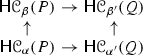
We end this section with another Rips zigzag construction similar to the image Čech zigzag. It consists of a nested pair of Morozov zigzags with multipliers $\rho \ge \eta \ge 0$. Canonical inclusions between Rips complexes give the following commutative diagram at the homology level:

$$\begin{aligned} \begin{array}{ccccccccc} \cdots &{} \leftarrow &{} \mathsf {H}{\mathcal {R}}_{\rho \varepsilon _i}(P_i) &{} \rightarrow &{} \mathsf {H}{\mathcal {R}}_{\rho \varepsilon _i}(P_{i+1}) &{} \leftarrow &{} \mathsf {H}{\mathcal {R}}_{\rho \varepsilon _{i+1}}(P_{i+1}) &{} \rightarrow &{} \cdots \\ &{}&{} \uparrow &{}&{} \uparrow &{}&{} \uparrow &{}\\ \cdots &{} \leftarrow &{} \mathsf {H}{\mathcal {R}}_{\eta \varepsilon _i}(P_i) &{} \rightarrow &{} \mathsf {H}{\mathcal {R}}_{\eta \varepsilon _i}(P_{i+1}) &{} \leftarrow &{} \mathsf {H}{\mathcal {R}}_{\eta \varepsilon _{i+1}}(P_{i+1}) &{} \rightarrow &{} \cdots \end{array} \end{aligned}$$

The vertical arrows in this diagram form a module homomorphism from the M-ZZ with multiplier $\eta$ to the M-ZZ with multiplier $\rho$. The image Rips zigzag (iR-ZZ) is defined as the image of this homomorphism. It is written as follows, where each $\mathsf {H}{\mathcal {R}}_{\eta \varepsilon _r}^{\rho \varepsilon _r}(P_s)$ denotes the image of the map $\mathsf {H}{\mathcal {R}}_{\eta \varepsilon _r}(P_s)\rightarrow \mathsf {H}{\mathcal {R}}_{\rho \varepsilon _r}(P_s)$:

$$\begin{aligned} \cdots \leftarrow {\mathcal {R}}_{\eta \varepsilon _{i}}^{\rho \varepsilon _i}(P_{i}) \rightarrow {\mathcal {R}}_{\eta \varepsilon _{i}}^{\rho \varepsilon _{i}}(P_{i+1}) \leftarrow {\mathcal {R}}_{\eta \varepsilon _{i+1}}^{\rho \varepsilon _{i+1}}(P_{i+1}) \rightarrow \cdots \end{aligned}$$

Image Rips zigzags have been available in the Dionysus library [16] since early 2009, with no theoretical guarantee on their behavior. Here we provide a guarantee on the output that is similar to the one obtained in Theorem 4.2 for the oscillating Rips zigzag.

Theorem 4.7

Let $\rho$ and $\eta$ be multipliers such that $\rho >10$ and $\frac{3}{\vartheta _{d}} <\eta < \frac{\rho -4}{2\vartheta _{d}}$. Let $X\subset \mathbb {R}^d$ be a compact set, let $P\subset \mathbb {R}^d$be a finite set, and let $\varepsilon = \mathrm {d}_H(P,X)$. Then, for any $l>k$ such that

$$\begin{aligned}&\max \left\{ \frac{3\varepsilon }{\vartheta _{d}\eta -3},\; \frac{4\varepsilon }{\rho -2\vartheta _{d}\eta -4}\right\} \le \varepsilon _l\\&\qquad \qquad \le \varepsilon _k < \min \left\{ \frac{1}{6}\mathrm {wfs}(X)-\varepsilon ,\;\frac{1}{\vartheta _{d}\rho +1} \left( \mathrm {wfs}(X)-\varepsilon \right) \right\} , \end{aligned}$$

the iR-ZZ restricted to $\mathsf {H}{\mathcal {R}}_{\eta \varepsilon _k}^{\rho \varepsilon _k}(P_{k+1}) \leftarrow \cdots \leftarrow \mathsf {H}{\mathcal {R}}_{\eta \varepsilon _l}^{\rho \varepsilon _l}(P_l)$ contains only isomorphisms, and its spaces are isomorphic to $\mathsf {H}X^\lambda$ for any $\lambda \in (0, \mathrm {wfs}(X))$. Therefore, its persistence barcode is made only of full-length intervals whose number equals the dimension of $\mathsf {H}X^\lambda$.

Proof

Our hypotheses imply $\frac{\rho }{2}\ge \vartheta _{d}\eta$, so we can use (1) to obtain the following diagram, where all arrows are canonical inclusions:

$$\begin{aligned} \begin{array}{ccccccccc} \cdots &{} \leftarrow &{} {\mathcal {C}}_{\vartheta _{d}\rho \varepsilon _i}(P_i) &{} \rightarrow &{} {\mathcal {C}}_{\vartheta _{d}\rho \varepsilon _i}(P_{i+1}) &{} \leftarrow &{} {\mathcal {C}}_{\vartheta _{d}\rho \varepsilon _{i+1}}(P_{i+1}) &{} \rightarrow &{} \cdots \\ &{}&{} \uparrow &{}&{} \uparrow &{}&{} \uparrow &{}\\ \cdots &{} \leftarrow &{}~ {\mathcal {R}}_{\rho \varepsilon _i}(P_i) &{} \rightarrow &{}~ {\mathcal {R}}_{\rho \varepsilon _i}(P_{i+1}) &{} \leftarrow &{}~ {\mathcal {R}}_{\rho \varepsilon _{i+1}}(P_{i+1}) &{} \rightarrow &{} \cdots \\ &{}&{} \uparrow &{}&{} \uparrow &{}&{} \uparrow &{}\\ \cdots &{} \leftarrow &{}~ {\mathcal {C}}_{\frac{\rho }{2}\varepsilon _i}(P_i) &{} \rightarrow &{}~ {\mathcal {C}}_{\frac{\rho }{2}\varepsilon _i}(P_{i+1}) &{} \leftarrow &{}~ {\mathcal {C}}_{\frac{\rho }{2}\varepsilon _{i+1}}(P_{i+1}) &{} \rightarrow &{} \cdots \\ &{}&{} \uparrow &{}&{} \uparrow &{}&{} \uparrow &{}\\ \cdots &{} \leftarrow &{} {\mathcal {C}}_{\vartheta _{d}\eta \varepsilon _i}(P_i) &{} \rightarrow &{} {\mathcal {C}}_{\vartheta _{d}\eta \varepsilon _i}(P_{i+1}) &{} \leftarrow &{} {\mathcal {C}}_{\vartheta _{d}\eta \varepsilon _{i+1}}(P_{i+1}) &{} \rightarrow &{} \cdots \\ &{}&{} \uparrow &{}&{} \uparrow &{}&{} \uparrow &{}\\ \cdots &{} \leftarrow &{}~ {\mathcal {R}}_{\eta \varepsilon _i}(P_i) &{} \rightarrow &{}~ {\mathcal {R}}_{\eta \varepsilon _i}(P_{i+1}) &{} \leftarrow &{}~ {\mathcal {R}}_{\eta \varepsilon _{i+1}}(P_{i+1}) &{} \rightarrow &{} \cdots \\ &{}&{} \uparrow &{}&{} \uparrow &{}&{} \uparrow &{}\\ \cdots &{} \leftarrow &{}~ {\mathcal {C}}_{\frac{\eta }{2}\varepsilon _i}(P_i) &{} \rightarrow &{}~ {\mathcal {C}}_{\frac{\eta }{2}\varepsilon _i}(P_{i+1}) &{} \leftarrow &{}~ {\mathcal {C}}_{\frac{\eta }{2}\varepsilon _{i+1}}(P_{i+1}) &{} \rightarrow &{} \cdots \end{array} \end{aligned}$$

This diagram induces a homomorphism $\Phi$ from the iR-ZZ ${\mathbb {U}}$ of parameters $\eta ,\rho$ to the image Čech zigzag ${\mathbb {V}}$ of parameters $\vartheta _{d}\eta ,\vartheta _{d}\rho$. Call ${\mathbb {U}}^*$ (resp. ${\mathbb {V}}^*$) the restriction of ${\mathbb {U}}$ (resp. ${\mathbb {V}}$) to the scale range $[(\varepsilon _k, P_{k+1}),\ (\varepsilon _l, P_l)]$. The restriction of $\Phi$ to ${\mathbb {U}}^*$ is an isomorphism onto ${\mathbb {V}}^*$. To see this, pick an arbitrary index $i$ in the range $[k+1,l]$ and consider the following sequence of inclusions between Čech complexes:

$$\begin{aligned} {\mathcal {C}}_{\frac{\eta }{2}\varepsilon _i}(P_{i}) \mathop {\longrightarrow }\limits ^{a} {\mathcal {C}}_{\vartheta _{d}\eta \varepsilon _i}(P_{i}) \mathop {\longrightarrow }\limits ^{b} {\mathcal {C}}_{\frac{\rho }{2}\varepsilon _i}(P_{i}) \mathop {\longrightarrow }\limits ^{c} {\mathcal {C}}_{\vartheta _{d}\rho \varepsilon _i}(P_{i+1}). \end{aligned}$$

Under our geometric hypotheses, it follows from Theorem 2.5 (i) that the maps $c\circ b\circ a$ and $b$ induce homomorphisms of the same rank at the homology level. Since $a$ and $c$ factor through Rips complexes as shown previously, rank inequalities induced by composition imply that the map $\mathsf {H}{\mathcal {R}}_{\eta \varepsilon _i}^{\rho \varepsilon _i}(P_i) \rightarrow \mathsf {H}{\mathcal {C}}_{\vartheta _{d}\eta \varepsilon _i}^{\vartheta _{d}\rho \varepsilon _i}(P_i)$ is an isomorphism. The same argument holds for the map $\mathsf {H}{\mathcal {R}}_{\eta \varepsilon _i}^{\rho \varepsilon _i}(P_{i+1}) \rightarrow \mathsf {H}{\mathcal {C}}_{\vartheta _{d}\eta \varepsilon _i}^{\vartheta _{d}\rho \varepsilon _i}(P_{i+1})$, with $i\in [k,l-1]$. Thus, the restriction of $\Phi$ to ${\mathbb {U}}^*$ is indeed an isomorphism onto ${\mathbb {V}}^*$. The conclusion of the theorem follows because the spaces in ${\mathbb {V}}^*$ are isomorphic to $\mathsf {H}X^\lambda$ and the maps in ${\mathbb {V}}^*$ are isomorphisms, as guaranteed by Theorem 4.1. $\square$

5 Complexity Bounds

We assume that the ordering of the points of $P$ is by furthest point sampling.⁴ Then every prefix $P_i$ is an $\varepsilon _i$-sparse $\varepsilon _i$-sample of $P$, and so standard ball packing arguments like that used in [19, Lemma 4.1] can be applied to bound the memory usage and running times of our Rips zigzags. The corresponding bounds are given below. Note that they are stated in terms of the doubling dimension of the input point set because it may be smaller than the ambient Euclidean dimension and thus gives sharper bounds.

5.1 Memory Usage

The relevant parameter here is the multiplier $\rho$, which conditions the size of the biggest complex in a Rips zigzag.

Theorem 5.1

Suppose $P$ is sitting in some metric space of doubling dimension $d$. Then, for any $k\ge 0$, the number of $k$-simplices in the current complex at any time of the construction of the M-ZZ of parameter $\rho$ is at most $2^{O(kd\log \rho )} n$, where $n$ is the cardinality of $P$. The same bound applies to the oR-ZZ and iR-ZZ of parameter $\rho$, regardless of the value of the parameter $\eta \le \rho$. Finally, given a constant $\zeta \in (0,1]$ and indices $n_1 = 1$ and $n_{i+1} = \min \{j>n_i\mid \varepsilon _j \le \zeta \varepsilon _{n_i}\}$, the number of $k$-simplices in any complex of the dM-ZZ is at most $2^{O(kd\log \frac{\rho }{\zeta })}n$.

Proof

We prove the result in the case of the dM-ZZ; the other cases follow by letting $\zeta =1$. Let $1=n_1 < n_2 < \cdots < n_{r-1} < n_r$ be the discretization indices. Since each prefix $P_{n_i}$ is $\varepsilon _{n_i}$-sparse, a standard ball-packing argument shows that every point $p\in P_{n_i}$ is connected to at most $2^{O(d\log \rho )}$ neighbors in the Rips complex ${\mathcal {R}}_{\rho \varepsilon _{n_i}}(P_{n_i})$. These neighbors can form at most $\left( \begin{array}{c}2^{O(d\log \rho )} \\ k\end{array}\right) = 2^{O(kd\log \rho )}$ k-simplices with p. Thus, the total number of k-simplices in ${\mathcal {R}}_{\rho \varepsilon _{n_i}}(P_{n_i})$ is at most $2^{O(kd\log \rho )}n_i \le 2^{O(kd\log \rho )} n$.

Let us now bound the size of ${\mathcal {R}}_{\rho \varepsilon _{n_i}}(P_{n_{i+1}})$. It follows from the definition of $n_{i+1}$ that $P_{n_{i+1}-1}$ is $\zeta \varepsilon _{n_i}$-sparse. Then the same ball-packing argument as previously shows that every point $p\in P$ has at most $2^{O(d\log \frac{\rho }{\zeta })}$ points of $P_{n_{i+1}-1}$ within distance $\rho \varepsilon _{n_i}$. Applying this result to every $p\in P_{n_{i+1}}$, and observing that the set difference $P_{n_{i+1}} \setminus P_{n_{i+1}-1}$ consists only of the point $p_{n_{i+1}}$, we deduce that every vertex of ${\mathcal {R}}_{\rho \varepsilon _{n_i}}(P_{n_{i+1}})$ has at most $2^{O(d\log \frac{\rho }{\zeta })}$ neighbors, as previously. The rest of the analysis follows. $\square$

Since the theoretical lower bounds on $\rho$ derived in Sect. 4 are constant ($\rho > 10$), one is allowed to set $\rho$ to some constant value in practice and benefit from our guarantees on the quality of the output. Meanwhile, Theorem 5.1 ensures that the number of $k$-simplices in the current complex remains at most $2^{O(kd)}n$ throughout the construction of the M-ZZ, oR-ZZ, or iR-ZZ. When using the dM-ZZ, one can also set $\zeta$ to be a constant as in (12), thereby benefiting from the theoretical guarantees on the quality of the output while maintaining the number of $k$-simplices in the current complex below $2^{O(kd)}n$ throughout the construction of the zigzag. Note, however, that the exact complex size is bigger than the one achieved with the other types of Rips zigzags when $\zeta <1$. These asymptotic bounds are as good in order of magnitude as those achieved with previous lightweight structures [15, 27].

5.2 Runtime

In experiments, we observed a significant slowdown in the running time of the oR-ZZ compared to the M-ZZ, iR-ZZ, and dM-ZZ. This is a result of the oR-ZZ inserting and removing the same simplices many times. Thus, the total number of insertions is a relevant indicator of running time, and it is driven by the value of $\eta$: the closer it is to $\rho$, the fewer simplex insertions and deletions occur during the zigzag calculation.

Theorem 5.2

Suppose $P$ is sitting in some metric space of doubling dimension $d$. Then, for any $k\ge 0$, the total number of $k$-simplices inserted in the current complex throughout the construction of the M-ZZ of parameter $\rho$ is at most $2^{O(kd\log \rho )} n$, where $n$ is the cardinality of $P$. The same bound applies to the iR-ZZ of parameter $\rho$, regardless of the value of parameter $\eta \le \rho$. For the oR-ZZ of parameters $\eta ,\rho$, the bound becomes $2^{O(kd\log \rho )} n^2$. Finally, given a constant $\zeta \in (0,1]$ and indices $n_1 = 1$ and $n_{i+1} = \min \{j>n_i \mid \varepsilon _j \le \zeta \varepsilon _{n_i}\}$, the bound for the dM-ZZ is $2^{O(kd\log \frac{\rho }{\zeta })}n$.

Proof

We begin with the M-ZZ, for which we will use a simple charging argument. Observe that simplex insertions occur only when a forward arrow is encountered in the zigzag. For any such arrow, the current complex is enlarged by adding a new vertex $p_{i+1}$ and connecting it to the rest of the complex. By the same packing argument as in the proof of Theorem 5.1, $p_{i+1}$ forms at most $2^{O(d\log \rho )}$ edges with the points of $P_i$; therefore, the number of $k$-simplices in its star in ${\mathcal {R}}_{\rho \varepsilon _i}(P_{i+1})$ is at most $2^{O(kd\log \rho )}$. This is also the number of $k$-simplices created at this stage of the algorithm. Hence, the total number of $k$-simplices inserted throughout the process is at most $2^{O(kd\log \rho )} n$. This bound applies also to the iR-ZZ, which maintains two Morozov zigzags: one of parameter $\rho$, the other of parameter $\eta \le \rho$.

The case of the dM-ZZ is similar, with the additional twist that more than one vertex is added to the current complex when going from ${\mathcal {R}}_{\rho \varepsilon _{n_i}}(P_{n_i})$ to ${\mathcal {R}}_{\rho \varepsilon _{n_i}}(P_{n_{i+1}})$. Nevertheless, as observed in the proof of Theorem 5.1, the points of $P_{n_{i+1}-1}$ are $\zeta \varepsilon _{n_i}$-sparse, so the number of edges in the star of any point of $P_{n_{i+1}}$ in ${\mathcal {R}}_{\rho \varepsilon _{n_i}}(P_{n_{i+1}})$ is at most $2^{O(d\log \frac{\rho }{\zeta })}$, and the number of $k$-simplices is bounded by $2^{O(kd\log \frac{\rho }{\zeta })}$. Hence, the total number of $k$-simplices inserted at this stage of the algorithm is at most $2^{O(d\log \frac{\rho }{\zeta })} (n_{i+1}-n_i)$. The result follows.

Finally, the case of the oR-ZZ with parameters $\eta <\rho$ is trickier. Due to the fact that both the vertex set and the Rips parameter increase when a forward arrow is encountered in the zigzag, we cannot simply charge the new simplex insertions to the newly added vertices: former vertices also form new simplices together. In fact, our bound is obtained by a cruder argument: for any forward arrow, the current complex contains at most $2^{O(kd\log \rho )} n$ k-simplices before and after following the arrow. Hence, in the worst case, the complex is rebuilt entirely, which means inserting at most $2^{O(kd\log \rho )} n$ k-simplices in total. Since this is true for any of the $n-1$ forward arrows, the claimed quadratic bound follows. $\square$

6 Experiments

Our implementation of the Rips zigzags of Sect. 4 is available as a package (called homology-zigzags) of the C++ library Dionysus [16].

6.1 Manufactured Data

As a proof of concept, we ran our code on the so-called Clifford data set from [22], which was obtained by evenly spacing 2,000 points along the line $l:y = 20 x \mod 2\pi$ in the second flat torus $(\mathbb {R}\mod 2\pi )^2$, then mapping the points onto the Clifford torus in $\mathbb {R}^4$ via the embedding $f:(u,v)\mapsto (\cos u,\; \sin u,\; \cos v,\; \sin v)$. This data set admits three nontrivial candidate underlying spaces: at small scales, the image of $l$ through $f$, which is a closed helicoidal curve on the torus; at larger scales, the torus itself; at even larger scales, the 3-sphere of radius $\sqrt{2}$ on which the torus is sitting.

We ran the M-ZZ, dM-ZZ, iR-ZZ, and oR-ZZ using the parameter values given in Table 1. Although these values lie outside the intervals prescribed by the theory, they were sufficient to obtain good results in practice. The corresponding results for the M-ZZ and dM-ZZ are reported in Figs. 1 and 2, respectively. The barcodes are represented on a logarithmic geometric scale (i.e., the horizontal axis shows the value of $\log _2 \varepsilon _i$), with ephemeral (length zero) intervals removed for clarity. The results obtained with the iR-ZZ and oR-ZZ are similar to Fig. 2 and therefore omitted.

The three spaces underlying the input data (curve, torus, 3-sphere) appear in all these barcodes; meanwhile, the topological noise remains small (M-ZZ) or even ephemeral (dM-ZZ, iR-ZZ, oR-ZZ). Of particular interest is the 3-sphere, whose corresponding 3-homology cycle appears only at large scales and for a short while because the 3-sphere is not densely sampled by the point cloud. This delicate 3-cycle certainly exists in the barcode of the standard Rips filtration; however, it cannot be observed in practice. As mentioned in [22], the union of balls of radius $\alpha$ around the data points covers the entire sphere only for $\alpha \ge \sqrt{4-2\sqrt{2}}$, so the corresponding 3-homology cycle can appear in the Rips filtration only at a parameter value $\alpha \ge \frac{\sqrt{4-2\sqrt{2}}}{\vartheta _{d}}>\sqrt{2}$. Now, a simulation reveals that the 4-skeleton of the Rips complex at such parameter values contains more than 31 billion simplices, a size that lies at least two orders of magnitude beyond the sizes currently handled by existing implementations. On a 24-GB machine we were able to store the 4-skeleton of the Rips filtration and compute its persistent homology within the main memory up to $\alpha \approx 0.625$ using Dionysus. The corresponding truncated barcode is represented on a $\log _2$ scale in Fig. 3. As expected, it shows only the curve and the torus, not the 3-sphere.

Fig. 1

Barcode of M-ZZ

Fig. 2

Barcode of dM-ZZ

Fig. 3

Barcode of standard Rips filtration

Table 1 Maximum complex size (in number of simplices) and total number of simplex insertions

For comparison we recall in Fig. 4 the barcode obtained by Hudson et al. using their mesh-based filtration [22]. Although the scale has been adapted so that it is the same as in the previous figures, any direct comparison of the barcodes should be made with the caveat that the intervals are half-open as in [22], rather than closed as in the present paper. Nevertheless, the general trend here is that, although the three spaces underlying the input data do appear in the barcode, the amount of noise is significant and its structure is quite irregular, despite the regularity of the data. Most notably, the amplitude of the noise in 1- or 2-homology is larger than the amplitude of the signal in 3-homology, which tends to obscure the information carried within the barcode. The superiority of Rips zigzags over mesh-based filtrations can also be stated in terms of efficiency: as reported in [22], the mesh-based filtration contains 12 million simplices, whereas our Rips zigzags contain less than 200,000 simplices at any given time (Table 1). The oR-ZZ did perform over seven million simplex insertions and deletions in total; however, the other zigzags performed much fewer such operations, as predicted by Theorem 5.2. In practice, computing any of our Rips zigzags together with its barcode took only a few minutes on a single Intel Xeon CPU core running at 2.40 GHz, whereas computing the mesh-based filtration and its barcode took hours on a similar architecture.

Fig. 4

Barcode of mesh-based filtration

6.2 Real Data

To demonstrate the practicality of our approach, we applied it to a real-life example derived from the statistics of natural images. The data set, described by Lee et al. in [25], consists of $4.2$ million high-contrast log-intensity $3\times 3$ patches extracted from van Hateren’s collection of still images [28]. Each patch is normalized in such a way that it can be represented as a point on the unit sphere $\mathbb {S}^7$ in the Euclidean space $\mathbb {R}^8$.

This eight-dimensional data set was studied in depth by Carlsson and coauthors [6, 12], who used the witness complex filtration to analyze its topological structure. Their findings led them to conjecture that the data were concentrated mostly around three circles with four points of intersection, as depicted in Fig. 5a. To uncover this structure, they applied several statistical filters to the point cloud (henceforth called $P$):

• 1. Since the focus was primarily on high-density areas of the data, they thresholded $P$ by density using the $k$th nearest neighbor density estimator, keeping only the fraction $x$ of the data points with lowest $k$th nearest neighbor distance. Varying $k$ from 1,200 to 24,000 and $x$ from 10 to 30 %, they obtained a collection $P_{k,x}$ of high-density subsets of $P$.

  Fig. 5

  

  Experimental results from [12] (images courtesy of G. Carlsson and V. de Silva). a Three-circle  model. b Barcode obtained with $k=1{,}200$ and $x=30\,\%$. c Barcode obtained with $k=24{,}000$ and $x=30\,\%$

• 2. Considering each set $P_{k,x}$ independently, they selected a subset $W_{k,x}$ of 5,000 random points sampled uniformly, which they took as their witness set.

• 3. Among the points of $W_{k,x}$ they selected a subset $L_{k,x}$ of 50 landmarks by a furthest-point sampling strategy.

After this preprocessing phase, they computed the barcode of the witness complex filtration for each pair $(L_{k,x}, W_{k,x})$ independently. Their results in 1-homology show two trends:

• For smaller values of $k$, the barcodes reveal five long bars – see, for example, Fig. 5b – corresponding to the homology of the three-circle model of Fig. 5a.

• For larger values of $k$, the barcodes reveal only one long bar – see, for example, Fig. 5c – suggesting that one of the circles is prevailing over the other two, which once again corroborates the three-circle model as depicted in Fig. 5a.

In [6], the authors also conjectured that the three circles might actually lie on a Klein bottle. Their intuition came from the observation that the three circles could be combined into a natural parameterization of the space of high-contrast $3\times 3$ patches that has the topology of a Klein bottle. Unfortunately, as intellectually satisfying as this hypothesis may be, they were not able to verify it beyond any doubt in practice, as it took them a fair amount of tweaking to make the Klein bottle appear in their barcodes. One possible explanation is that they were using too few landmarks in an attempt to prevent the size of the witness complex filtration from becoming intractable. The question of the size and choice of the landmark set affects the validity of their experimental results as a whole since, after all, there are not many shapes out there that can be faithfully sampled with only 50 points. Thus, even their results in 1-homology call for further experimental validation.

Our Rips zigzags are particularly relevant for this validation. Using the same preprocessed data, we took the whole set $W_{k,x}$ as landmarks and computed the persistence (up to seven dimensions) of their associated Morozov zigzags. We subsampled the data down to 500 points to compute the diagrams for dimensions 4 and higher. This took less than 1 h per data set and used less than 2 GB of RAM. The barcodes obtained for $W_{k,x}$ with $(k=1,200,\ x=30)$ and $(k=24{,}000,\ x=30)$ are shown in Figs. 6 and 7, respectively. While they do corroborate the results of Fig. 5, they show a clear absence of any higher-dimensional topological structure. This further strengthens the three-circle model hypothesis while weakening the Klein bottle model hypothesis. It does not discard the latter entirely, though, since our results are subject to the initial density filtering step, which might be too rough in its current form. A more subtle statistical preprocessing of the data might change the situation,⁵ and so the question of the presence (or not) of the Klein bottle in this data set is left open.

Fig. 6

Barcode of M-ZZ of $W_{k,x}$ with $k=1{,}200$ and $x=30$

Fig. 7

Barcode of M-ZZ of $W_{k,x}$ with $k=24{,}000$ and $x=30$

7 Discussion

In this paper, we explored several Rips zigzags that achieve both small size and bounded topological noise for homology inference. While our size bounds are comparable to those obtained in previous work, our bounds on the noise are clearly better since they guarantee the noise is either totally absent or just ephemeral. Our proofs rely on general new techniques for manipulating and comparing zigzag modules. We hope that these techniques will find further use and stimulate new research and applications of zigzag persistence. For now we provide an in-depth discussion of the potential and limitations of our results.

7.1 Choosing Among Rips Zigzags in Practice

Each one of our zigzags has its own strengths and weaknesses, whether in terms of output quality or in terms of computing efficiency. Table 2 summarizes their theoretical behavior with respect to the key aspects of our analysis: length of sweet range, amplitude of topological noise, memory usage, and running time versus number of input points.

Table 2 Theoretical behavior of Rips zigzags of Sect. 4

This table shows a clear advantage of the iR-ZZ and should encourage the user to prefer it over the other zigzags in practice. However, it is somewhat misleading because only the asymptotic memory usage and running time bounds are given. In fact, maintaining two M-ZZs requires up to twice the amount of memory required to maintain just one, which makes a huge difference on some data sets, including in terms of actual running time. Moreover, the iR-ZZ requires an implementation of the zigzag persistence algorithm for images, a version that is likely to be less efficient than its nonimage counterpart. For instance, in our experiments on the Clifford data set the iR-ZZ was ten times slower to compute than the M-ZZ.

Among the other zigzags, the oR-ZZ clearly gives the best results in terms of quality, both in theory and in practice. Unfortunately, its computation turns out to be much slower than those of the other zigzags. In our experiments the slow-down factor compared to the M-ZZ went up to thousands.

The discretized M-ZZ achieves a good tradeoff between running time and output quality. In our experiments, the running times were comparable to that of the M-ZZ (only slower by a factor of two at most), while the output barcodes contained much less topological noise. A shortcoming, though, is that large discretization steps tend to oversimplify the barcodes, sometimes treating some relevant yet delicate topological features as noise and removing the corresponding bars in the output. Such issues occur less often with the other zigzags, which insert the data points one by one instead of in batches.

Thus, as a general rule of thumb, we suggest using the M-ZZ first in practice when dealing with a new data set. This is especially true if the data are supposed to be sampled from so-called simple shapes (e.g., ones with positive reach or $\mu$-reach), in which case the quality of the output should be comparable to that achieved with the other zigzags (albeit with a smaller sweet range). Then, in cases where the quality of the result is not sufficient and one needs to obtain cleaner (less noisy) barcodes, either one of the three variants may be considered: dM-ZZ, oR-ZZ, or iR-ZZ. Although we did prefer the dM-ZZ for its good tradeoff in general, in some specific scenarios, the iR-ZZ or oR-ZZ was definitely the better choice.

7.2 Beyond Euclidean Spaces

The geometric part of our analysis of the Rips zigzags of Sect. 4 assumes that the vertex set is sitting in some Euclidean space, Hausdorff-close to some compact set. This hypothesis is made for the sake of convenience because it allows us to refer to the sampling theory for compact sets developped by Chazal and coauthors [7]. However, it does not reflect the variety of scenarios in which Rips zigzags can be used.

Since their construction only requires a matrix of pairwise distances as input, Rips zigzags are applicable in any metric space. Although they come with no theoretical guarantees in such a generality, there are many contexts in which some things can be said about their persistence barcodes. Finite samples of a compact subset of $\mathbb {R}^d$ is but one example. Another important example is when $P$ is sampled from a compact Riemannian manifold or, more generally, from a compact Alexandrov space with curvature bounded from above, or, even more generally, from any compact length space $X$ with positive convexity radius; see, for example, [3] for an introduction to these spaces. It is beyond the scope of this paper to redo our analysis in this context; however, for completeness we provide high-level directions on how to adapt it:

• Compact spaces with a positive convexity radius admit finite covers with (small enough) convex metric balls, so the Nerve Lemma and its persistent variant hold. One can then reproduce the results of Sect. 2.2, and in particular Theorem 2.5, with $X$ being the whole space instead of some compact subset, and with the convexity radius of $X$ playing the role formerly played by the weak feature size.⁶ This settles most of the geometric aspects of the analysis of Sect. 4.

• The one part of the analysis that remains to be adapted is when the results by Attali et al. [1] are invoked to bound the amplitude of the noise in the barcode of the M-ZZ. These results require $P$ to be sitting close to some compact set with positive $\mu$-reach in $\mathbb {R}^d$. However, it turns out that they follow previous work by Hausmann [21] and Latschev [24], which focuses precisely on cases where $P$ lies on Riemannian manifolds or more general length spaces and whose results apply directly to the present context.

• Once these geometric aspects have been adapted, the rest of the analysis can be reproduced and theorems similar to those of Sect. 4 can be derived for the oR-ZZ, M-ZZ, dM-ZZ, and iR-ZZ. While the lower bounds of the sweet ranges still depend on the sampling density parameter $\varepsilon$, the upper bounds now depend on the convexity radius rather than on the weak feature size.

7.3 Zigzag Manipulations and Functoriality

The topological part of our analysis of Rips zigzags relies on manipulating zigzags via arrow reversals or space removals, and of paramount importance is the fact that such manipulations can be performed while preserving (most of) the internal structure of the zigzags as well as the commutativity of the diagrams. In a sense, one can see the Arrow Reversal and Space Removal Theorems as providing operators from the class of zigzags of a certain type $\tau$ to the class of zigzags of another type $\tau ^*$. In the arrow reversal case, $\tau$ and $\tau ^*$ differ by a single arrow orientation, while in the space removal case they differ by a single space. An important question is to understand when and why these operators would preserve commutativity, which can be cast mathematically into the question of whether these operators can be made functorial.

To formalize this question, we use the language of quiver theory, in which a module type $\tau$ is called a quiver and is represented as a directed graph whose undirected version is a simple path, as in the following example:

$$\begin{aligned} \bullet \longrightarrow \bullet \longleftarrow \bullet \longrightarrow \bullet \longrightarrow \bullet \end{aligned}$$

A zigzag module ${\mathbb {V}}$ of type $\tau$ is called a representation of $\tau$. The class of all representations of $\tau$, together with the module homomorphisms connecting them, forms a category denoted by $\mathrm {Rep}_{\tau }$. In the case of arrow reversals, we are given another module type $\tau ^*$ that differs from $\tau$ by a single arrow orientation, and we ask ourselves whether there exist functors $\mathrm{F }: \mathrm {Rep}_{\tau }\rightarrow \mathrm {Rep}_{\tau ^*}$ that preserve the interval decompositions of $\tau$’s representations, i.e.,

$$\begin{aligned} \forall {\mathbb {V}}\in \mathrm {Rep}_{\tau },\ \mathsf {Pers}({\mathbb {V}}) = \mathsf {Pers}(\mathrm{F }({\mathbb {V}})). \end{aligned}$$

(13)

Beyond the question of the existence of such functors (which remains a mystery to us at present) lies that of their intrinsic properties. Considering that the arrow reversal operator is naturally reversible (applying it twice to a module ${\mathbb {V}}$ gives either ${\mathbb {V}}$ itself or some module isomorphic to it, depending on the choice of isomorphism in the Interval Decomposition Theorem 2.6), it is desireable that the functor $\mathrm{F }$ also be reversible in some sense. There exist many notions of reversibility for functors in the theory of categories, and here we check $\mathrm{F }$ against the following classical notions: (a) isomorphism of categories, (b) equivalence of categories, (c) left or right adjoint. There is a natural gradation between these concepts: isomorphisms are equivalences and equivalences are adjoint.

We show in the appendix that, given $\tau ,\tau ^*$ as previously, there is no covariant functor $\mathrm{F }:\mathrm {Rep}_{\tau }\rightarrow \mathrm {Rep}_{\tau ^*}$ of type (a), (b), or (c) that satisfies (13). In other words, there is no hope of finding reversible covariant arrow-reversing functors that preserve persistence diagrams, at least for the aforementioned classical notions of functor reversibility. We also show that a similar conclusion holds for contravariant functors, under the extra hypothesis that the length of $\tau ,\tau ^*$ (i.e., the number of nodes in the graph) is at least 3 and not just 2. Indeed, for module types of length 2, plain vector space duality induces a contravariant functor that is an isomorphism of categories.

These negative results regarding the functoriality of arrow reversals are a pretty bad piece of news. And unfortunately, claims of a similar flavor can be made for space removals as well.⁷ This being said, we have only scratched the surface of the problem so far. For instance, we still do not know whether functors satisfying (13) exist. Further investigations should be conducted to assess the real potential of the arrow reversal and space removal operators to derive more canonical variants and to make connections with other operations on quivers such as, for instance, reflection and Coxeter functors [2].

Appendix: Functoriality

To prove that no functor of type (c) exists – and thus no functor of type (a) or (b) either – we use the fact that left (resp. right) adjoint functors are right (resp. left) exact, i.e., they preserve right (resp. left) exact sequences [23, §3.3.6].

Lemma 8.1

Let $\tau ,\tau ^*$ be module types of length at least 2 that differ by a single arrow orientation. Then, there is no covariant functor $\mathrm{F }:\mathrm {Rep}_{\tau }\rightarrow \mathrm {Rep}_{\tau ^*}$ satisfying (13) that is either left or right exact.

Proof

By the restriction principle, we only need to focus on module types of length 2. Then let $\tau$ be the quiver $\bullet \longrightarrow \bullet$ and $\tau ^*$ the quiver $\bullet \longleftarrow \bullet$. Suppose that there exists a covariant functor $\mathrm{F }:\mathrm {Rep}_{\tau }\rightarrow \mathrm {Rep}_{\tau ^*}$ that satisfies (13). Then consider the following sequence of module homomorphisms (drawn horizontally) connecting various representations of $\tau$ (drawn vertically upwards), where $\varvec{k}$ denotes the field of coefficients:

$$\begin{aligned} \begin{array}{ccccccccc} 0 &{} \mathop {\longrightarrow }\limits ^{0} &{} \varvec{k}&{} \mathop {\longrightarrow }\limits ^{{1\!\!1}} &{} \varvec{k}&{} \mathop {\longrightarrow }\limits ^{0} &{} 0 &{} \mathop {\longrightarrow }\limits ^{0} &{} 0 \\ \uparrow \scriptstyle {0} &{} &{} \uparrow \scriptstyle {0} &{} &{} \uparrow \scriptstyle {{1\!\!1}} &{} &{} \uparrow \scriptstyle {0} &{} &{} \uparrow \scriptstyle {0} \\ 0 &{} \mathop {\longrightarrow }\limits ^{0} &{} 0 &{} \mathop {\longrightarrow }\limits ^{0} &{} \varvec{k}&{} \mathop {\longrightarrow }\limits ^{{1\!\!1}} &{} \varvec{k}&{} \mathop {\longrightarrow }\limits ^{0} &{} 0 \end{array} \end{aligned}$$

It is easily seen that this sequence is exact. By (13) it is sent to a sequence of the following form through $\mathrm{F }$, where the spaces $A,B,C,D$ are isomorphic to $\varvec{k}$:

$$\begin{aligned} \begin{array}{ccccccccc} 0 &{} \mathop {\longrightarrow }\limits ^{0} &{} A &{} \mathop {\longrightarrow }\limits ^{0} &{} C &{} \mathop {\longrightarrow }\limits ^{0} &{} 0 &{} \mathop {\longrightarrow }\limits ^{0} &{} 0 \\ \downarrow \scriptstyle {0} &{} &{} \downarrow \scriptstyle {0} &{} &{} \downarrow \scriptstyle {\cong } &{} &{} \downarrow \scriptstyle {0} &{} &{} \downarrow \scriptstyle {0} \\ 0 &{} \mathop {\longrightarrow }\limits ^{0} &{} 0 &{} \mathop {\longrightarrow }\limits ^{0} &{} B &{} \mathop {\longrightarrow }\limits ^{0} &{} D &{} \mathop {\longrightarrow }\limits ^{0} &{} 0 \end{array} \end{aligned}$$

Note that the map $A\longrightarrow C$ must be zero for the quadrant $A,C,B,0$ to commute. Likewise, the map $B\longrightarrow D$ must be zero for the quadrant $C,0,D,B$ to commute. Thus, this new sequence is neither left nor right exact. $\square$

Lemma 8.2

Let $\tau ,\tau ^*$ be module types of length at least 3 that differ by a single arrow orientation. Then, there is no contravariant functor $\mathrm{F }:\mathrm {Rep}_{\tau }\rightarrow \mathrm {Rep}_{\tau ^*}$ satisfying (13) that is either left or right exact.

Proof

By the restriction principle, we need only focus on module types of length 3. Then let $\tau$ be the quiver $\bullet \longrightarrow \bullet \longleftarrow \bullet$ and $\tau ^*$ the quiver $\bullet \longrightarrow \bullet \longrightarrow \bullet$, the other option ($\tau =\bullet \longleftarrow \bullet \longrightarrow \bullet$ and $\tau ^*=\bullet \longrightarrow \bullet \longrightarrow \bullet$) being similar and left as an exercise. Suppose that there exists a contravariant functor $\mathrm{F }:\mathrm {Rep}_{\tau }\rightarrow \mathrm {Rep}_{\tau ^*}$ that satisfies (13). Then consider the following sequence of module homomorphisms (drawn horizontally) connecting various representations of $\tau$ (drawn vertically upwards), where $\varvec{k}$ denotes the field of coefficients:

It is easily seen that this sequence is exact. By (13) it is sent to a sequence of the following form through $\mathrm{F }$, where the spaces $A,B,C,D,E,F$ are isomorphic to $\varvec{k}$:

$$\begin{aligned} \begin{array}{ccccccccc} 0 &{} \mathop {\longleftarrow }\limits ^{0} &{} 0 &{} \mathop {\longleftarrow }\limits ^{0} &{} D &{} \longleftarrow &{} F &{} \mathop {\longleftarrow }\limits ^{0} &{} 0 \\ \uparrow \scriptstyle {0} &{} &{} \uparrow \scriptstyle {0} &{} &{} \uparrow \scriptstyle {\cong } &{} &{} \uparrow \scriptstyle {0} &{} &{} \uparrow \scriptstyle {0} \\ 0 &{} \mathop {\longleftarrow }\limits ^{0} &{} A &{} \mathop {\longleftarrow }\limits ^{0} &{} C &{} \mathop {\longleftarrow }\limits ^{0} &{} 0 &{} \mathop {\longleftarrow }\limits ^{0} &{} 0 \\ \uparrow \scriptstyle {0} &{} &{} \uparrow \scriptstyle {0} &{} &{} \uparrow \scriptstyle {\cong } &{} &{} \uparrow \scriptstyle {0} &{} &{} \uparrow \scriptstyle {0} \\ 0 &{} \mathop {\longleftarrow }\limits ^{0} &{} 0 &{} \mathop {\longleftarrow }\limits ^{0} &{} B &{} \mathop {\longleftarrow }\limits ^{0} &{} E &{} \mathop {\longleftarrow }\limits ^{0} &{} 0 \end{array} \end{aligned}$$

Note that the map $A\longleftarrow C$ must be zero for the quadrant $A,C,B,0$ to commute. Likewise, the map $B\longleftarrow E$ must be zero for the quadrant $C,0,E,B$ to commute. Thus, this new sequence is neither left nor right exact. $\square$

References

D. Attali, A. Lieutier, and D. Salinas. Vietoris-Rips complexes also provide topologically correct reconstructions of sampled shapes. Computational Geometry: Theory and Applications, 46(4):448–465, 2012.
I. N. Bernstein, I. M. Gelfand, and V. A. Ponomarev. Coxeter functors and Gabriel’s theorem. Russian Mathematical Surveys, 28(2):17–32, 1973.
D. Burago, Y. Burago, and S. Ivanov. A Course in Metric Geometry, volume 33 of Graduate Studies in Mathematics. American Mathematical Society, Providence, RI, 2001.
G. Carlsson. Topology and data. Bulletin of the American Mathematical Society, 46(2):255–308, 2009.
G. Carlsson and V. de Silva. Zigzag persistence. Foundations of Computational Mathematics, 10(4):367–405, 2010.
G. Carlsson, T. Ishkhanov, V. de Silva, and A. Zomorodian. On the local behavior of spaces of natural images. Int. J. Comput. Vision, 76(1):1–12, January 2008.
F. Chazal and D. Cohen-Steiner. Geometric inference. In Tesselations in the Sciences. Springer-Verlag, 2013.
F. Chazal, D. Cohen-Steiner, and A. Lieutier. A sampling theory for compact sets in Euclidean space. Discrete & Computational Geometry, 41:461–479, 2009.
F. Chazal, L. J. Guibas, S. Y. Oudot, and P. Skraba. Analysis of scalar fields over point cloud data. Discrete and Computational Geometry, 46(4):743–775, December 2011.
F. Chazal and S. Y. Oudot. Towards persistence-based reconstruction in Euclidean spaces. In Proc. 24th ACM Symposium on Computational Geometry, pages 232–241, 2008.
V. de Silva. A weak characterisation of the Delaunay triangulation. Geometriae Dedicata, 135(1):39–64, August 2008.
V. de Silva and G. Carlsson. Topological estimation using witness complexes. IEEE Symposium on Point-based Graphic, pages 157–166, 2004.
V. de Silva and R. Ghrist. Coverage in sensor networks via persistent homology. Algebraic and Geometric Topology, 7:339–358, 2007.
T. K. Dey, F. Fan, and Y. Wang. Graph induced complex on point data. In Proc. 29th Annual Symposium on Computational Geometry, pages 107–116, New York, NY, USA, 2013. ACM.
Tamal K. Dey, Fengtao Fan, and Yusu Wang. Computing topological persistence for simplicial maps. In Proc. 30th Annual Symposium on Computational Geometry, 2014.
Dionysus. By D. Morozov (http://www.mrzv.org/software/dionysus/).
H. Edelsbrunner, D. Letscher, and A. Zomorodian. Topological persistence and simplification. Discrete and Computational Geometry, 28:511–533, 2002.
P. Gabriel. Unzerlegbare Darstellungen I. Manuscripta Mathematica, 6:71–103, 1972.
L. J. Guibas and S. Y. Oudot. Reconstruction using witness complexes. Discrete and Computational Geometry, 40(3):325–356, 2008.
A. Hatcher. Algebraic Topology. Cambridge Univ. Press, 2001.
J.-C. Hausmann. On the Vietoris-Rips complexes and a cohomology theory for metric spaces. Prospects in topology, Ann. of Math. Stud., 138:175–188, 1995.
B. Hudson, G. Miller, S. Y. Oudot, and D. Sheehy. Topological inference via meshing. In Proc. ACM Symposium on Computational geometry, pages 277–286. ACM, 2010.
M. Kashiwara and P. Schapira. Categories and Sheaves, volume 332 of Grundlehren der mathematischen Wissenschaften. Springer-Verlag, 2006.
J. Latschev. Vietoris-Rips complexes of metric spaces near a closed Riemannian manifold. Archiv der Mathematik, 77(6):522–528, 2001.
A. B. Lee, K. S. Pedersen, and D. Mumford. The nonlinear statistics of high-contrast patches in natural images. Int. J. Comput. Vision, 54(1–3):83–103, August 2003.
D. Morozov. Personal communication.
D. R. Sheehy. Linear-size approximations to the vietoris-rips filtration. In Proc. ACM Symposium on Computational Geometry, pages 239–248. ACM, 2012.
J. H. van Hateren and A. van der Schaaff. Independent component filters of natural images compared with simple cells in primary visual cortex. Proceedings of the Royal Society, London, B, 265:359–366, 1997.
A. Zomorodian and G. Carlsson. Computing persistent homology. Discrete Comput. Geom., 33(2):249–274, 2005.
Acknowledgments
The authors wish to thank the referees for their careful reading of the paper and their insightful comments. They also thank Marc Glisse for suggesting the approach used in the proof of Theorem 4.3, Frédéric Chazal and Vin de Silva for helpful discussions, and Dmitriy Morozov for agreeing to integrate their code into the Dionysus library. This work was supported by the European Project CG-Learning 255827 and by the ANR project TopData.
Author information
Authors and Affiliations
Corresponding author
Additional information
Communicated by Herbert Edelsbrunner.