Transaction costs, trading volume, and the liquidity premium

Abstract

In a market with one safe and one risky asset, an investor with a long horizon, constant investment opportunities and constant relative risk aversion trades with small proportional transaction costs. We derive explicit formulas for the optimal investment policy, its implied welfare, liquidity premium, and trading volume. At the first order, the liquidity premium equals the spread, times share turnover, times a universal constant. The results are robust to consumption and finite horizons. We exploit the equivalence of the transaction cost market to another frictionless market, with a shadow risky asset, in which investment opportunities are stochastic. The shadow price is also found explicitly.

1 Introduction

If risk aversion and investment opportunities are constant—and frictions are absent—investors should hold a constant mix of safe and risky assets [30–32]. Transaction costs substantially change this statement, casting some doubt on its far-reaching implications.¹ Even the small spreads that are present in the most liquid markets entail wide oscillations in portfolio weights, which imply variable risk premia.

This paper studies a tractable benchmark of portfolio choice under transaction costs, with constant investment opportunities, summarized by a safe rate r, and a risky asset with volatility σ and expected excess return μ>0, which trades at a bid (selling) price (1−ε)S _t equal to a constant fraction (1−ε) of the ask (buying) price S _t . Our analysis is based on the model of Dumas and Luciano [12], which concentrates on long-run asymptotics to gain in tractability. In their framework, we find explicit solutions for the optimal policy, welfare, liquidity premium² and trading volume, in terms of model parameters, and of an additional quantity, the gap, identified as the solution to a scalar equation. For all these quantities, we derive closed-form asymptotics, in terms of model parameters only, for small transaction costs.

We uncover novel relations among the liquidity premium, trading volume, and transaction costs. First, we show that share turnover ($\operatorname{ShTu}$), the liquidity premium ($\operatorname{LiPr}$), and the bid-ask spread ε satisfy the asymptotic relation

$$ \operatorname{LiPr}\approx\frac{3}{4} \varepsilon \operatorname{ShTu}. $$

This relation is universal, as it involves neither market nor preference parameters. Also, because it links the liquidity premium, which is unobservable, with spreads and share turnover, which are observable, this relation can help estimate the liquidity premium using data on trading volume.

Second, we find that the liquidity premium behaves very differently in the presence of leverage. In the no-leverage regime, the liquidity premium is an order of magnitude smaller than the spread [7], as unlevered investors respond to transaction costs by trading infrequently. With leverage, however, the liquidity premium increases quickly, because rebalancing a levered position entails high transaction costs, even under the optimal trading policy.

Third, we obtain the first continuous-time benchmark for trading volume, with explicit formulas for share and wealth turnover. Trading volume is an elusive quantity for frictionless models, in which turnover is typically infinite in any time interval.³ In the absence of leverage, our results imply low trading volume compared to the levels observed in the market. Of course, our model can only explain trading generated by portfolio rebalancing, and not by other motives such as market timing, hedging, and life-cycle investing.

Moreover, welfare, the liquidity premium, and trading volume depend on the market parameters (μ,σ) only through the mean-variance ratio μ/σ ² if measured in business time, that is, using a clock that ticks at the speed of the market’s variance σ ². In usual calendar time, all these quantities are in turn multiplied by the variance σ ².

Our main implication for portfolio choice is that a symmetric, stationary policy is optimal for a long horizon, and it is robust, at the first order, both to intermediate consumption, and to a finite horizon. Indeed, we show that the no-trade region is perfectly symmetric with respect to the Merton proportion π _∗=μ/γσ ², if trading boundaries are expressed with trading prices, that is, if the buy boundary π ₋ is computed from the ask price, and the sell boundary π ₊ from the bid price.

Since the optimal policy in a frictionless market is independent both of intermediate consumption and of the horizon (cf. Merton [31]), our results entail that these two features are robust to small frictions. However plausible these conclusions may seem, the literature so far has offered diverse views on these issues (cf. Davis and Norman [9], Dumas and Luciano [12], as well as Liu and Loewenstein [25]). More importantly, robustness to the horizon implies that the long-horizon approximation, made for the sake of tractability, is reasonable and relevant. For typical parameter values, we see that our optimal strategy is nearly optimal already for horizons as short as two years.

A key idea for our results—and for their proof—is the equivalence between a market with transaction costs and constant investment opportunities, and another shadow market, without transaction costs, but with stochastic investment opportunities driven by a state variable. This state variable is the ratio between the investor’s risky and safe weights, which tracks the location of the portfolio within the trading boundaries, and affects both the volatility and the expected return of the shadow risky asset.

In this paper, using a shadow price has two related advantages over alternative methods: first, it allows us to tackle the issue of verification with duality methods developed for frictionless markets. These duality methods in turn yield the finite-horizon bounds in Theorem 3.1 below, which measure the performance of long-run policies over a given horizon—an issue that is especially important when an asymptotic objective function is used. The shadow price method was applied successfully by Kallsen and Muhle-Karbe [24] as well as Gerhold et al. [16, 17] for logarithmic utility, and this paper brings this approach to power utility, which allows to understand how optimal policies, welfare, liquidity premia and trading volume depend on risk aversion. The recent papers of Herzegh and Prokaj [22] as well as Choi et al. [6] consider power utility from consumption over an infinite horizon.

The paper is organized as follows. Section 2 introduces the portfolio choice problem and states the main results. The model’s main implications are discussed in Sect. 3, and the main results are derived heuristically in Sect. 4. Section 5 concludes, and all proofs are in the Appendices A, B and C.

2 Model and main result

Consider a market with a safe asset earning an interest rate r, i.e., $S^{0}_{t}=e^{rt}$, and a risky asset trading at ask (buying) price S _t following geometric Brownian motion,

$$ dS_t/S_t=(\mu+r)\, dt+\sigma dW_t. $$

Here, W is a standard Brownian motion, μ>0 is the expected excess return,⁴ and σ>0 is the volatility. The corresponding bid (selling) price is (1−ε)S _t , where ε∈(0,1) represents the relative bid-ask spread.

A self-financing trading strategy is a two-dimensional, predictable process (φ ⁰,φ) of finite variation, such that $\varphi^{0}_{t}$ and φ _t represent the number of units in the safe and risky asset at time t, and the initial number of units is $(\varphi^{0}_{0-},\varphi_{0-}){=}(\xi^{0},\xi) {\in}\mathbb {R}^{2}_{+}\backslash \{0,0\}$. Writing $\varphi_{t} = \varphi^{\uparrow}_{t}-\varphi ^{\downarrow }_{t}$ as the difference between the cumulative number of shares bought ($\varphi^{\uparrow}_{t}$) and sold ($\varphi^{\downarrow}_{t}$) by time t, the self-financing condition relates the dynamics of $\varphi^{0}_{t}$ and φ _t via

$$ d\varphi^0_t = -\frac{S_t}{S^0_t}\, d\varphi_t^{\uparrow}+ (1-\varepsilon )\frac{S_t}{S^0_t}\, d\varphi^{\downarrow}_t . $$

(2.1)

As in Dumas and Luciano [12], the investor maximizes the equivalent safe rate of power utility, an optimization objective that also proved useful with constraints on leverage (cf. Grossman and Vila [18]) and drawdowns (see Grossman and Zhou [19]).

Definition 2.1

A trading strategy $(\varphi^{0}_{t},\varphi_{t})$ is admissible if its liquidation value is positive, in the sense that

$$ \varXi^\varphi_t=\varphi^0_t S^0_t+(1-\varepsilon)S_t\varphi_t^+ -\varphi_t^- S_t\ge0, \quad\text{a.s. for all }t\ge0. $$

An admissible strategy $(\varphi^{0}_{t},\varphi_{t})$ is long-run optimal if it maximizes the equivalent safe rate

$$ \liminf_{T \to\infty} \frac{1}{T}\log E\big[(\varXi^\varphi_T)^{1-\gamma}\big]^{\frac{1}{1-\gamma}} $$

(2.2)

over all admissible strategies, where 1≠γ>0 denotes the investor’s relative risk aversion.⁵

Our main result is the following:

Theorem 2.2

Suppose an investor with constant relative risk aversion γ>0 trades to maximize (2.2). Then, for small transaction costs ε>0:

• (i) (Equivalent safe rate)

  For the investor, trading the risky asset with transaction costs is equivalent to leaving all wealth in a hypothetical safe asset, which pays the higher equivalent safe rate

  $$ \operatorname{ESR}=r+\frac{\mu^2-\lambda^2}{2\gamma\sigma^2}, $$

  where the gap λ is defined in (iv) below.

• (ii) (Liquidity premium)

  Trading the risky asset with transaction costs is equivalent to trading a hypothetical asset, at no transaction costs, with the same volatility σ, but with lower expected excess return $\sqrt{\mu^{2}-\lambda^{2}}$. Thus, the liquidity premium is

  $$ \operatorname{LiPr}= \mu-\sqrt{\mu^2-\lambda^2}. $$

• (iii) (Trading policy)

  It is optimal to keep the fraction of wealth held in the risky asset within the buy and sell boundaries

  $$ \pi_-=\frac{\mu-\lambda}{\gamma\sigma^2}, \qquad \pi_+=\frac{\mu+\lambda}{\gamma\sigma^2}, $$

  (2.3)

  where the risky weights π ₋ and π ₊ are computed with ask and bid prices, respectively.⁶

• (iv) (Gap)

  For μ/γσ ²≠1, the constant λ≥0 is the unique value for which the solution of the initial value problem

  

  also satisfies the terminal condition

  $$ w\left(\log\frac{u(\lambda)}{\ell(\lambda)} \right) = \frac{\mu +\lambda}{\gamma\sigma^2}, \quad\text{\textit{where} } \frac{u(\lambda)}{\ell(\lambda)} = \frac{1}{ 1-\varepsilon}\frac {(\mu +\lambda)(\mu-\lambda-\gamma\sigma^2)}{(\mu-\lambda)(\mu+\lambda-\gamma\sigma^2)}. $$

  In view of the explicit formula for w(x,λ) in Lemma A.1 below, this is a scalar equation for λ. For μ/γσ ²=1, the gap λ vanishes.

• (v) (Trading volume)

  Let μ≠σ ²/2.⁷ Then share turnover, which is here defined as shares traded $d\|\varphi\|_{t}=d\varphi ^{\uparrow}_{t}+d\varphi^{\downarrow}_{t}$ divided by shares held |φ _t |, has the long-term average

  

  Wealth turnover, defined as wealth traded divided by wealth held, has the long-term average ⁸

  

• (vi) (Asymptotics)

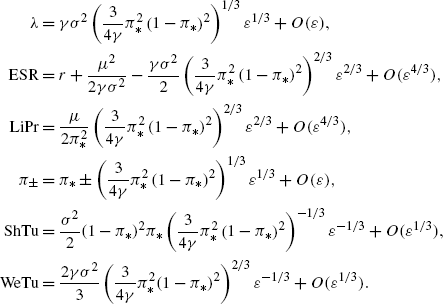
  Setting π _∗=μ/γσ ², the following expansions in terms of the bid-ask spread ε hold:⁹

  

  (2.4)

In summary, our optimal trading policy and its resulting welfare, liquidity premium and trading volume are all simple functions of investment opportunities (r, μ and σ), preferences (γ) and the gap λ. The gap does not admit an explicit formula in terms of the transaction cost parameter ε, but is determined through the implicit relation in (iv), and has the asymptotic expansion in (vi), from which all other asymptotic expansions follow through the explicit formulas.

The frictionless markets with constant investment opportunities in (i) and (ii) of Theorem 2.2 are equivalent to the market with transaction costs in terms of equivalent safe rates. Nevertheless, the corresponding optimal policies are very different, requiring no or incessant rebalancing in the frictionless markets of (i) and (ii), respectively, whereas there is finite positive trading volume in the market with transaction costs.

By contrast, the shadow price, which is key in the derivation of our results, is a fictitious risky asset, with price evolving within the bid-ask spread, for which the corresponding frictionless market is equivalent to the transaction cost market in terms of both welfare and the optimal policy.

Theorem 2.3

The policy in Theorem 2.2(iii) and the equivalent safe rate in Theorem 2.2(i) are also optimal for a frictionless asset with shadow price $\tilde{S}_{t}$, which always lies within the bid-ask spread and coincides with the trading price at times of trading for the optimal policy. The shadow price satisfies

$$ d\tilde{S}_t/\tilde{S}_t = \big(\tilde{\mu}(\varUpsilon_t)+r\big)\,dt + \tilde{\sigma}(\varUpsilon_t) \,dW_t, $$

for the deterministic functions $\tilde{\mu}(\cdot)$ and $\tilde{\sigma }(\cdot)$ given explicitly in Lemma B.2. The state variable $\varUpsilon_{t}=\log(\varphi_{t} S_{t}/({\ell(\lambda)}\varphi ^{0}_{t} S^{0}_{t}))$ represents the logarithm of the ratio of risky and safe positions, which follows a Brownian motion with drift, reflected to remain in the interval [0,log(u(λ)/ℓ(λ))], i.e.,

$$ d\varUpsilon_t=(\mu-\sigma^2/2)\,dt+\sigma \,dW_t +dL_t-dU_t. $$

Here, L _t and U _t are increasing processes, proportional to the cumulative purchases and sales, respectively (cf. (B.9) below). In the interior of the no-trade region, that is, when ϒ _t lies in (0,log(u(λ)/ℓ(λ))), the numbers of units of the safe and risky asset are constant, and the state variable ϒ _t follows Brownian motion with drift. As ϒ _t reaches the boundary of the no-trade region, buying or selling takes place so as to keep it within [0,log(u(λ)/ℓ(λ))].

In view of Theorem 2.3, trading with constant investment opportunities and proportional transaction costs is equivalent to trading in a fictitious frictionless market with stochastic investment opportunities, which vary with the location of the investor’s portfolio in the no-trade region.

3 Implications

3.1 Trading strategies

Equation (2.3) implies that trading boundaries are symmetric around the frictionless Merton proportion π _∗=μ/γσ ². At first glance, this seems to contradict previous studies (e.g. Liu and Loewenstein [25], Shreve and Soner [35]), which emphasize how these boundaries are asymmetric, and may even fail to include the Merton proportion. These papers employ a common reference price (the average of the bid and ask prices) to evaluate both boundaries. By contrast, we express trading boundaries using trading prices (i.e., the ask price for the buy boundary, and the bid price for the sell boundary). This simple convention unveils the natural symmetry of the optimal policy, and explains asymmetries as figments of notation—even in their models. To see this, denote by $\pi_{-}'$ and $\pi_{+}'$ the buy and sell boundaries in terms of the ask price. These papers prove the bounds (Shreve and Soner [35, (11.4) and (11.6)] in an infinite-horizon model with consumption, resp. Liu and Loewenstein [25, (22), (23)] in a finite-horizon model)

$$ \pi_-'< \frac{\mu}{\gamma\sigma^2} \quad\text{and}\quad \frac{\mu}{\gamma\sigma^2(1-\varepsilon)+\varepsilon\mu} < \pi_+' < \frac{\mu}{\frac{1}{2}\gamma\sigma^2(1-\varepsilon )+\varepsilon \mu} . $$

(3.1)

With trading prices (i.e., substituting $\pi_{-}=\pi_{-}'$ and $\pi _{+}=\frac {1-\varepsilon}{1-\varepsilon\pi_{+}'}\pi_{+}'$), these bounds become

$$ \pi_-< \frac{\mu}{\gamma\sigma^2} < \pi_+ < 2\frac{\mu}{\gamma\sigma^2}, $$

(3.2)

whence the Merton proportion always lies between π ₋ and π ₊.

To understand the robustness of our optimal policy to intermediate consumption, we compare our trading boundaries with those obtained by Davis and Norman [9] as well as Shreve and Soner [35] in the consumption model of Magill and Constantinides [29]. The asymptotic expansions of Janeček and Shreve [23] make this comparison straightforward.

With or without consumption, the trading boundaries coincide at the first order. This fact has a clear economic interpretation: The separation between consumption and investment, which holds in a frictionless model with constant investment opportunities, is a robust feature of frictionless models, because it still holds, at the first order, even with transaction costs. Put differently, if investment opportunities are constant, consumption has only a second order effect for investment decisions, in spite of the large no-trade region implied by transaction costs. Figure 1 shows that our bounds are very close to those obtained in the model of Davis and Norman [9] for bid-ask spreads below 1 %, but start diverging for larger values.

Fig. 1

Buy (lower) and sell (upper) boundaries (vertical axis, as risky weights) as functions of the spread ε, in linear scale (upper panel) and cubic scale (lower panel). The plot compares the approximate weights from the first term of the expansion (dotted), the exact optimal weights (solid), and the boundaries found by Davis and Norman [9] in the presence of consumption (dashed). Parameters are μ=8 %, σ=16 %, γ=5, and a zero discount rate for consumption (for the dashed curve)

3.2 Business time and mean-variance ratio

In a frictionless market, the equivalent safe rate and the optimal policy are

$$\operatorname{ESR}= r + \frac{1}{2\gamma} \left(\frac{\mu}{\sigma}\right)^2 \quad\text{and}\quad \pi_* = \frac{\mu}{\gamma\sigma^2}. $$

This rate depends only on the safe rate r and the Sharpe ratio μ/σ. Investors are indifferent between two markets with identical safe rates and Sharpe ratios, because both markets lead to the same set of payoffs, even though a payoff is generated by different portfolios in the two markets. By contrast, the optimal portfolio depends only on the mean-variance ratio μ/σ ².

With transaction costs, (2.4) shows that the asymptotic expansion of the gap per unit of variance λ/σ ² only depends on the mean-variance ratio μ/σ ². Put differently, holding the mean-variance ratio μ/σ ² constant, the expansion of λ is linear in σ ². In fact, not only the expansion but also the exact quantity has this property, since λ/σ ² in (iv) only depends on μ/σ ².

Consequently, the optimal policy in (iii) only depends on the mean-variance ratio μ/σ ², as in the frictionless case. The equivalent safe rate, however, no longer solely depends on the Sharpe ratio μ/σ: Investors are not indifferent between two markets with the same Sharpe ratio, because one market is more attractive than the other if it entails lower trading costs. As an extreme case, in one market it may be optimal to leave all wealth in the risky asset, eliminating any need to trade. Instead, the formulas in (i), (ii) and (v) show that like the gap per variance λ/σ ², the equivalent safe rate, the liquidity premium, and both share and wealth turnover only depend on μ/σ ², when measured per unit of variance. The interpretation is that these quantities are proportional to business time σ ² t (compare Ané and Geman [2]), and the factor of σ ² arises from measuring them in calendar time.

In the frictionless limit, the linearity in σ ² and the dependence on μ/σ ² cancel, and the result depends on the Sharpe ratio alone. For example, the equivalent safe rate becomes¹⁰

$$r+\frac{\sigma^2}{2\gamma} \left(\frac{\mu}{\sigma^2}\right)^2 =r+\frac {1}{2\gamma}\left(\frac{\mu}{\sigma}\right)^2 . $$

3.3 Liquidity premium

The liquidity premium [7] is the amount of expected excess return the investor is ready to forgo to trade the risky asset without transaction costs, so as to achieve the same equivalent safe rate. Figure 2 plots the liquidity premium against the spread ε (upper panel) and risk aversion γ (lower panel).

Fig. 2

Upper panel: liquidity premium (vertical axis) against the spread ε, for risk aversion γ equal to 5 (solid), 1 (long dashed), and 0.5 (short dashed). Lower panel: liquidity premium (vertical axis) against risk aversion γ, for spread ε=0.01 % (solid), 0.1 % (long dashed), 1 % (short dashed), and 10 % (dotted). Parameters are μ=8 % and σ=16 %

The liquidity premium is exactly zero when the Merton proportion π _∗ is either zero or one. In these two limit cases, it is optimal not to trade at all, hence no compensation is required for the costs of trading. The liquidity premium is relatively low in the regime of no leverage (0<π _∗<1), corresponding to γ>μ/σ ², confirming the results of Constantinides [7], who reports liquidity premia one order of magnitude smaller than trading costs.

The leverage regime (γ<μ/σ ²), however, shows a very different picture. As risk aversion decreases below the full-investment level γ=μ/σ ², the liquidity premium increases rapidly towards the expected excess return μ, as lower levels of risk aversion prescribe increasingly high leverage. The costs of rebalancing a levered position are high, and so are the corresponding liquidity premia.

The liquidity premium increases in spite of the increasing width of the no-trade region for larger leverage ratios. In other words, even as a less risk averse investor tolerates wider oscillations in the risky weight, this increased flexibility is not enough to compensate for the higher costs required to rebalance a more volatile portfolio.

3.4 Trading volume

In the empirical literature (cf. Lo and Wang [26] and the references therein), the most common measure of trading volume is share turnover, defined as number of shares traded divided by shares held or, equivalently, as the value of shares traded divided by the value of shares held. In our model, turnover is positive only at the trading boundaries, while it is null inside the no-trade region. Since turnover, on average, grows linearly over time, we consider the long-term average of share turnover per unit of time, plotted in Fig. 3 against risk aversion. Turnover is null at the full-investment level γ=μ/σ ², as no trading takes place in this case. Lower levels of risk aversion generate leverage, and trading volume increases rapidly, like the liquidity premium.

Fig. 3

Trading volume (vertical axis, annual fractions traded), as share turnover (upper panel) and wealth turnover (lower panel), against risk aversion (horizontal axis), for spread ε=0.01 % (solid), 0.1 % (long dashed), 1 % (short dashed), and 10 % (dotted). Parameters are μ=8 % and σ=16 %

Share turnover does not decrease to zero as the risky weight decreases to zero for increasing risk aversion γ. On the contrary, the first term in the asymptotic formula converges to a finite level. This phenomenon arises because more risk averse investors hold less risky assets (reducing volume), but also rebalance more frequently (increasing volume). As risk aversion increases, neither of these effects prevails, and turnover converges to a finite limit.

To better understand these properties, consider wealth turnover, defined as the value of shares traded, divided by total wealth (not by the value of shares held).¹¹ Share and wealth turnover are qualitatively similar for low risk aversion, as the risky weight of wealth is larger, but they diverge as risk aversion increases and the risky weight declines to zero. Then, wealth turnover decreases to zero, whereas share turnover does not.

The levels of trading volume observed empirically imply very low values of risk aversion in our model. For example, Lo and Wang [26] report in the NYSE-AMEX an average weekly turnover of 0.78 % between 1962 and 1996, which corresponds to an approximate annual turnover above 40 %. As Fig. 3 shows, such a high level of turnover requires a risk aversion below 2, even for a very small spread of ε=0.01 %. Such a value cannot be interpreted as risk aversion of a representative investor, because it would imply a leveraged position in the stock market, which is inconsistent with equilibrium. This phenomenon intensifies in the last two decades. As shown by Fig. 4, turnover increases substantially from 1993 to 2010, with monthly averages of 20 % typical from 2007 on, corresponding to an annual turnover of over 240 %.

Fig. 4

Upper panel: share turnover (top), spread (center), and implied liquidity premium (bottom) in logarithmic scale, from 1992 to 2010. Lower panel: monthly averages for share turnover, spread, and implied liquidity premium over subperiods. Spread and turnover are capitalization-weighted averages across securities in the monthly CRSP database with share codes 10, 11 that have non-zero bid, ask, volume and shares outstanding

The overall implication is that portfolio rebalancing can generate substantial trading volume, but the model explains the trading volume observed empirically only with low risk aversion and high leverage. In a numerical study with risk aversion of 6 and spreads of 2 %, Lynch and Tan [28] also find that the resulting trading volume is too low, even allowing for labor income and predictable returns, and obtain a condition on the wealth-income ratio under which the trading volume has the same order of magnitude as reported by empirical studies. Our analytical results are consistent with their findings, but indicate that substantially higher volume can be explained with lower risk aversion, even in the absence of labor income.

3.5 Volume, spreads and the liquidity premium

The analogies between the comparative statics of the liquidity premium and trading volume suggest a close connection between these quantities. An inspection of the asymptotic formulas unveils the relations

$$ {\operatorname{LiPr}} = \frac{3}{4} \varepsilon{ \operatorname{ShTu}} + O(\varepsilon^{4/3}) \quad\text{and}\quad {\left(r+\frac{\mu^2}{2\gamma\sigma^2}\right)-\operatorname{ESR}} = \frac{3}{4} \varepsilon{ \operatorname{WeTu}} + O(\varepsilon^{4/3}). $$

(3.3)

These two relations have the same meaning: The welfare effect of small transaction costs is proportional to trading volume times the spread. The constant of proportionality 3/4 is universal, that is, independent of both investment opportunities (r, μ, σ) and preferences (γ).

In the first formula, the welfare effect is measured by the liquidity premium, that is, in terms of the risky asset. Likewise, trading volume is expressed as share turnover, which also focuses on the risky asset alone. By contrast, the second formula considers the decrease in the equivalent safe rate and wealth turnover, two quantities that treat both assets equally. In summary, if both welfare and volume are measured consistently with each other, the welfare effect approximately equals volume times the spread, up to the universal factor 3/4.

Figure 4 plots the spread, share turnover, and the liquidity premium implied by the first equation in (3.3). As in Lo and Wang [26], the spread and share turnover are capitalization-weighted averages of all securities in the Center for Research on Security Prices (CRSP) monthly stocks database with share codes 10 and 11, and with non-zero bid, ask, volume and share outstanding. While turnover figures are available before 1992, separate bid and ask prices were not recorded until then, thereby preventing a reliable estimation of spreads for earlier periods.

Spreads steadily decline in the observation period, dropping by almost an order of magnitude after stock market decimalization of 2001. At the same time, trading volume substantially increases from a typical monthly turnover of 6 % in the early 1990s to over 20 % in the late 2000s. The implied liquidity premium also declines with spreads after decimalization, but less than the spread, in view of the increase in turnover. During the months of the financial crisis in late 2008, the implied liquidity premium rises sharply, not because of higher volumes, but because spreads widen substantially. Thus, although this implied liquidity premium is only a coarse estimate, it has advantages over other proxies, because it combines information on both prices and quantities, and is supported by a model.

3.6 Finite horizons

The trading boundaries in this paper are optimal for a long investment horizon, but are also approximately optimal for finite horizons. The following theorem, which complements the main result, makes this point precise.

Theorem 3.1

Fix a time horizon T>0. Then the finite-horizon equivalent safe rate of any strategy $(\phi^{0}_{t},\phi_{t})$ satisfies the upper bound

(3.4)

and the finite-horizon equivalent safe rate of our long-run optimal strategy $(\varphi^{0}_{t} ,\varphi_{t})$ satisfies the lower bound

(3.5)

For the same unlevered initial position ($\phi_{0-}=\varphi_{0-}\ge0, \phi^{0}_{0-}=\varphi^{0}_{0-}\ge0$), the equivalent safe rates of $(\phi ^{0}_{t},\phi_{t})$ and of the optimal policy $(\varphi^{0}_{t},\varphi_{t})$ for horizon T therefore differ by at most

$$ \frac{1}{T} \Big(\log E\big[(\varXi^\phi_T)^{1-\gamma}\big]^{\frac {1}{1-\gamma}}- \log E\big[(\varXi^\varphi_T)^{1-\gamma}\big]^{\frac{1}{1-\gamma }}\Big)\le (3\pi_*+1)\frac{\varepsilon}{T}+O(\varepsilon^{4/3}). $$

(3.6)

This result implies that the horizon, like consumption, only has a second order effect on portfolio choice with transaction costs, because the finite-horizon equivalent safe rate matches, at the leading order ε ^2/3, the equivalent safe rate of the stationary long-run optimal policy. This result recovers in particular the first-order asymptotics for the finite-horizon value function obtained by Bichuch [4, Theorem 4.1]. In addition, Theorem 3.1 provides explicit estimates for the correction terms of order ε arising from liquidation costs. Indeed, $r+\frac {\mu^{2}-\lambda^{2}}{2\gamma\sigma^{2}}$ is the maximum rate achieved by trading optimally. The remaining terms arise due to the transient influence of the initial endowment, as well as the costs of the initial transaction, which takes place if the initial position lies outside the no-trade region, and of the final portfolio liquidation. These costs are of order ε/T because they are incurred only once, and hence defrayed by a longer trading period. By contrast, portfolio rebalancing generates recurring costs, proportional to the horizon, and their impact on the equivalent safe rate does not decline as the horizon increases.

Even after accounting for all such costs in the worst-case scenario, the bound in (3.6) shows that their combined effect on the equivalent safe rate is lower than the spread ε, as soon as the horizon exceeds 3π _∗+1, that is, four years in the absence of leverage. Yet, this bound holds only up to a term of order ε ^4/3, so it is worth comparing it with the exact bounds in (B.16), (B.17), from which (3.4) and (3.5) are obtained.

The exact bounds in Fig. 5 show that for typical parameter values, the loss in equivalent safe rate of the long-run optimal strategy is lower than the spread ε even for horizons as short as 18 months, and quickly declines to become ten times smaller, for horizons close to ten years. In summary, the long-run approximation is a useful modeling device that makes the model tractable, and the resulting optimal policies are also nearly optimal even for horizons of a few years.

Fig. 5

Upper bound on the difference between the long-run and finite-horizon equivalent safe rates (vertical axis), against the horizon (horizontal axis), for spread ε=0.01 % (solid), 0.1 % (long dashed), 1 % (short dashed), and 10 % (dotted). Parameters are μ=8 %, σ=16 %, γ=5

4 Heuristic solution

This section contains an informal derivation of the main results. Here, formal arguments of stochastic control are used to obtain the optimal policy, its welfare, and their asymptotic expansions.

4.1 Transaction costs market

For a trading strategy $(\varphi^{0}_{t},\varphi_{t})$, again write the number of risky shares $\varphi_{t}=\varphi_{t}^{\uparrow}-\varphi_{t}^{\downarrow}$ as the difference of the cumulated units purchased and sold, and denote by

$$X_t=\varphi^0_t S^0_t, \qquad Y_t=\varphi_t S_t, $$

the values of the safe and risky positions in terms of the ask price S _t . Then the self-financing condition (2.1) and the dynamics of $S^{0}_{t}$ and S _t imply

Consider the maximization of expected power utility U(x)=x ^1−γ/(1−γ) from terminal wealth at time T,¹² and denote by V(t,x,y) its value function, which depends on time and the value of the safe and risky positions. Itô’s formula yields

where the arguments of the functions are omitted for brevity. By the martingale optimality principle of stochastic control (cf. Davis and Varaiya [10]), the process V(t,X _t ,Y _t ) must be a supermartingale for any choice of the cumulative purchases and sales $\varphi^{\uparrow}_{t},\varphi^{\downarrow}_{t}$. Since these are increasing processes, it follows that V _y −V _x ≤0 and (1−ε)V _x −V _y ≤0, that is,

$$ 1 \le\frac{V_x}{V_y}\le\frac{1}{1-\varepsilon}. $$

In the interior of this “no-trade region”, where the number of risky shares remains constant, the drift of V(t,X _t ,Y _t ) cannot be positive, and must become zero for the optimal policy,¹³ so that

$$ V_t+ r x V_x+(\mu+r)y V_y+\frac{\sigma^2}{2} y^2 V_{yy} =0 \quad\text{if } 1< \frac{V_x}{V_y}<\frac{1}{1-\varepsilon}. $$

To simplify further, note that the value function must be homogeneous with respect to wealth, and that—in the long run—it should grow exponentially with the horizon at a constant rate. These arguments lead one to guess¹⁴ that

$$V(t,x,y)=x^{1-\gamma}v(y/x) e^{- (1-\gamma) (r+\beta) t} $$

for some β to be found. Setting z=y/x, the above equation reduces to

$$ \frac{\sigma^2}{2} z^2v''(z)+\mu z v'(z)- (1-\gamma) \beta v(z)=0 \quad\text{if } 1+z<\frac{ (1-\gamma) v(z)}{v'(z)}<\frac {1}{1-\varepsilon}+z. $$

(4.1)

Assuming that the no-trade region $\{z:1+z\leq\frac{ (1-\gamma) v(z)}{v'(z)}\leq\frac{1}{1-\varepsilon}+z\}$ coincides with some interval ℓ≤z≤u to be determined, and noting that at ℓ the left inequality in (4.1) holds as equality, while at u the right inequality holds as equality, the following free boundary problem arises:

(4.2)

(4.3)

(4.4)

These conditions are not enough to identify the solution, because they can be matched for any choice of the trading boundaries ℓ,u. The optimal boundaries are the ones that also satisfy the smooth-pasting conditions (cf. Beneš et al. [3], Dumas [11]), formally obtained by differentiating (4.3) and (4.4) with respect to ℓ and u, respectively. This gives

(4.5)

In addition to the reduced value function v, this system requires to solve for the excess equivalent safe rate β and the trading boundaries ℓ and u. Substituting (4.5) and (4.3) into (4.2) yields (cf. Dumas and Luciano [12])

Setting π ₋=ℓ/(1+ℓ), and factoring out (1−γ)v, it follows that

Note that π ₋ is the risky weight when it is time to buy, and hence the risky position is valued at the ask price. The same argument for u shows that the other solution of the quadratic equation is π ₊=u(1−ε)/(1+u(1−ε)), which is the risky weight when it is time to sell, and hence the risky position is valued at the bid price. Thus, the optimal policy is to buy when the “ask’’ fraction falls below π ₋, sell when the “bid’’ fraction rises above π ₊, and do nothing in between. Since π ₋ and π ₊ solve the same quadratic equation, they are related to β via

It is convenient to set β=(μ ²−λ ²)/2γσ ², because β=μ ²/2γσ ² without transaction costs. We call λ the gap, since λ=0 in a frictionless market, and, as λ increases, all variables diverge from their frictionless values. Put differently, to compensate for transaction costs, the investor would require another asset, with expected return λ and volatility σ, which trades without frictions and is uncorrelated with the risky asset.¹⁵ With this notation, the buy and sell boundaries are just

In other words, the buy and sell boundaries are symmetric around the classical frictionless solution μ/γσ ². Since ℓ(λ),u(λ) are identified by π _± in terms of λ, it now remains to find λ. After deriving ℓ(λ) and u(λ), the boundaries in the problem (4.2)–(4.4) are no longer free, but fixed. With the substitution

$$v(z)=e^{(1-\gamma)\int_0^{\log(z/{\ell(\lambda)})} w(y)\,dy}, \quad \mbox{i.e., } w(y)=\frac{{\ell(\lambda)}e^y v'({\ell(\lambda )}e^y)}{(1-\gamma)v({\ell(\lambda)}e^y)}, $$

the boundary problem (4.2)–(4.4) reduces to a Riccati ODE,

(4.6)

(4.7)

(4.8)

where y∈[0,logu(λ)/ℓ(λ)] and

$$ \frac{u(\lambda)}{\ell(\lambda)} = \frac{1}{1-\varepsilon}\frac{\pi_+ (1-\pi_-)}{\pi_- (1-\pi_+)} = \frac{1}{1-\varepsilon}\frac{(\mu+\lambda)(\mu-\lambda-\gamma \sigma^2)}{(\mu-\lambda)(\mu+\lambda-\gamma\sigma^2)}. $$

For each λ, the initial value problem (4.6), (4.7) has a solution w(λ,⋅), and the correct value of λ is identified by the second boundary condition (4.8).

4.2 Asymptotics

Equation (4.8) does not have an explicit solution, but it is possible to obtain an asymptotic expansion for small transaction costs (ε∼0) using the implicit function theorem. To this end, write the boundary condition (4.8) as f(λ,ε)=0, where

$$ f(\lambda,\varepsilon) = w\Big(\lambda, \log\big(u(\lambda )/{\ell (\lambda)}\big)\Big)-\frac{\mu+\lambda}{\gamma\sigma^2}. $$

Of course, f(0,0)=0 corresponds to the frictionless case. The implicit function theorem then suggests that around zero, λ(ε) follows the asymptotics λ(ε)∼−εf _ε /f _λ , but the difficulty is that f _λ =0, because λ is not of order ε. Heuristic arguments (cf. Shreve and Soner [35, Remark B.3], Rogers [34]) suggest that λ is of order ε ^1/3.¹⁶ Thus, setting λ=δ ^1/3 and $\hat{f}(\delta,\varepsilon)=f(\delta^{1/3},\varepsilon)$, and computing the derivatives of the explicit formula for w(λ,x) (cf. Lemma A.1) shows that

As a result, we obtain

$$ \delta(\varepsilon) \sim-\frac{f_\varepsilon}{f_\delta} \varepsilon= \frac{3 \mu^2 (\mu-\gamma\sigma^2 )^2}{4 \gamma^2 \sigma ^2}\varepsilon \quad\text{whence}\quad \lambda(\varepsilon) \sim \left(\frac{3\mu^2 \left(\mu-\gamma\sigma^2\right)^2}{4\gamma^2 \sigma^2}\right)^{1/3} \varepsilon^{1/3}. $$

The asymptotic expansions of all other quantities then follow by Taylor expansion.

5 Conclusion

In a tractable model of transaction costs with one safe and one risky asset and constant investment opportunities, we have computed explicitly the optimal trading policy, its welfare, liquidity premium, and trading volume, for an investor with constant relative risk aversion and a long horizon.

The trading boundaries are symmetric around the Merton proportion, if each boundary is computed with the corresponding trading price. Both the liquidity premium and the trading volume are small in the unlevered regime, but become substantial in the presence of leverage. For a small bid-ask spread, the liquidity premium is approximately equal to share turnover times the spread, times the universal constant 3/4.

Trading boundaries depend on investment opportunities only through the mean-variance ratio. The equivalent safe rate, the liquidity premium, and the trading volume also depend only on the mean-variance ratio if measured in business time.

Appendices

Appendix A: Explicit formulas and their properties

We now show that the candidate w for the reduced value function and the quantity λ are indeed well defined for sufficiently small spreads. The first step is to determine, for a given small λ>0, an explicit expression for the solution w of the ODE (4.6), complemented by the initial condition (4.7).

Lemma A.1

Let 0<μ/γσ ²≠1. Then for sufficiently small λ>0, the function

$$w(\lambda,y)= \begin{cases} \frac{a(\lambda)\tanh[\tanh^{-1}(b(\lambda)/a(\lambda ))-a(\lambda )y]+(\frac{\mu}{\sigma^2}-\frac{1}{2})}{\gamma-1},\\[5pt] \quad\mbox{\textit{if} } \gamma\in(0,1) \mbox{ \textit{and} } \frac {\mu}{\gamma\sigma^2}<1 \mbox{ \textit{or} } \gamma>1 \mbox{ \textit{and} } \frac {\mu}{\gamma\sigma^2}>1,\\[5pt] \frac{a(\lambda) \tan[\tan^{-1}(b(\lambda)/a(\lambda))+a(\lambda )y]+(\frac{\mu}{\sigma^2}-\frac{1}{2})}{\gamma-1},\\[5pt] \quad\mbox{\textit{if} } \gamma>1 \mbox{ \textit{and} } \frac{\mu }{\gamma\sigma^2} \in\left(\frac{1}{2}-\frac{1}{2}\sqrt{1-\frac {1}{\gamma}},\frac{1}{2}+\frac{1}{2}\sqrt{1-\frac{1}{\gamma }}\right),\\[5pt] \frac{a(\lambda)\coth[\coth^{-1}(b(\lambda)/a(\lambda))-a(\lambda )y]+(\frac{\mu}{\sigma^2}-\frac{1}{2})}{\gamma-1}, \\[5pt] \quad\mbox{\textit{otherwise}}, \end{cases} $$

with

$$a(\lambda)=\sqrt{\Big|(\gamma-1)\frac{\mu^2-\lambda^2}{\gamma \sigma ^4}-\Big(\frac{1}{2}-\frac{\mu}{\sigma^2}\Big)^2\Big|}, \qquad b(\lambda)=\frac{1}{2}-\frac{\mu}{\sigma^2}+(\gamma-1)\frac{\mu -\lambda}{\gamma\sigma^2}, $$

is a local solution of

$$ w'(y)+(1-\gamma)w^2(y)+\left(\frac{2\mu}{\sigma^2}-1\right)w(y)-\frac {\mu^2-\lambda^2}{\gamma\sigma^4}=0, \qquad w(0)=\frac{\mu-\lambda }{\gamma\sigma^2}. $$

(A.1)

Moreover, y↦w(λ,y) is increasing (resp. decreasing) for μ/γσ ²∈(0,1) (resp. μ/γσ ²>1).

Proof

The first part of the assertion is easily verified by taking derivatives, noticing that the case distinctions distinguish between the different signs of the discriminant

$$(\gamma-1)\frac{\mu^2-\lambda^2}{\gamma\sigma^4}-\left(\frac {1}{2}-\frac{\mu}{\sigma^2}\right)^2 $$

of the Riccati equation (A.1) for sufficiently small λ. Indeed, in the second case the discriminant is positive for sufficiently small λ. The first and third case correspond to a negative discriminant, as well as b(λ)/a(λ)<1 and b(λ)/a(λ)>1, respectively, for sufficiently small λ>0, so that the function w is well defined in each case.

The second part of the assertion follows by inspection of the explicit formulas. □

Next, we establish that the crucial constant λ, which determines both the no-trade region and the equivalent safe rate, is well defined.

Lemma A.2

Let 0<μ/γσ ²≠1 and w(λ,⋅) be defined as in Lemma A.1, and set

$${\ell(\lambda)}=\frac{\mu-\lambda}{\gamma\sigma^2-(\mu-\lambda )}, \qquad u(\lambda)=\frac{1}{1-\varepsilon}\frac{\mu+\lambda}{\gamma \sigma^2-(\mu +\lambda)}. $$

Then, for sufficiently small ε>0, there exists a unique solution λ of

$$ w\left(\lambda,\log\frac{u(\lambda)}{\ell(\lambda)} \right) -\frac{\mu+\lambda}{\gamma\sigma^2}=0. $$

(A.2)

As ε↓0, it has the asymptotics

Proof

The explicit expression for w in Lemma A.1 implies that w(λ,x) in Lemma A.1 is analytic in both variables at (0,0). By the initial condition in (A.1), its power series has the form

$$w(\lambda,x) = \frac{\mu-\lambda}{\gamma\sigma^2} +\sum_{i=1}^\infty\sum_{j=0}^\infty W_{ij} x^i \lambda^j, $$

where expressions for the coefficients W _ij are computed by expanding the explicit expression for w. (The leading terms are provided after this proof.) Hence, the left-hand side of the boundary condition (A.2) is an analytic function of ε and λ. Its power series expansion shows that the coefficients of ε ⁰ λ ^j vanish for j=0,1,2, so that the condition (A.2) reduces to

$$ \lambda^3 \sum_{i\geq0} A_i \lambda^i = \varepsilon\sum_{i,j\geq0} B_{ij} \varepsilon^i \lambda^j $$

(A.3)

with (computable) coefficients A _i and B _ij . This equation has to be solved for λ. Since

$$A_0 = \frac{4}{3\mu\sigma^2(\gamma\sigma^2-\mu)} \quad\text{and} \quad B_{00} = \frac{\mu(\gamma\sigma^2-\mu)}{\gamma^2\sigma^4} $$

are non-zero, divide (A.3) by ∑ _i≥0 A _i λ ⁱ, and take the third root, obtaining that, for some C _ij ,

$$\lambda= \varepsilon^{1/3} \sum_{i,j\geq0} C_{ij} \varepsilon^i \lambda^j = \varepsilon^{1/3} \sum_{i,j\geq0} C_{ij} (\varepsilon^{1/3})^{3i} \lambda^j . $$

The right-hand side is an analytic function of λ and ε ^1/3, so that the implicit function theorem [21, Theorem I.B.4] yields a unique solution λ (for ε sufficiently small), which is an analytic function of ε ^1/3. Its power series coefficients can be computed at any order. □

In the preceding proof, we needed the first coefficients of the series expansion of the analytic function on the left-hand side of (A.2). Calculating them is elementary, but rather cumbersome, and can be quickly performed with symbolic computation software. Following a referee’s suggestion, we present some expressions to aid readers who wish to check the calculations by hand, namely the derivatives of w at (λ,x)=(0,0) that are needed to calculate the Taylor coefficients of (A.2) used in the proof. Note that they are the same in all three cases of Lemma A.1, and given by

Henceforth, consider small transaction costs ε>0, and let λ denote the constant in Lemma A.2. Moreover, set w(y)=w(λ,y), a=a(λ), b=b(λ), and u=u(λ), ℓ=ℓ(λ). In all cases, the function w can be extended smoothly to an open neighborhood of [0,log(u/ℓ)] (resp. [log(u/ℓ),0] if μ/γσ ²>1). By continuity, the ODE (A.1) then also holds at 0 and log(u/ℓ); inserting the boundary conditions for w in turn readily yields the following counterparts for the derivative w′:

Lemma A.3

Let 0<μ/γσ ²≠1. Then, in all three cases,

$$w'(0)=\frac{\mu-\lambda}{\gamma\sigma^2}-\Bigg(\frac{\mu -\lambda}{\gamma \sigma^2}\Bigg)^2, \qquad w'\bigg(\log\frac{u}{\ell} \bigg)=\frac {\mu +\lambda}{\gamma\sigma^2}-\left(\frac{\mu+\lambda}{\gamma\sigma ^2}\right)^2. $$

Appendix B: Shadow prices and verification

The key to justify the heuristic arguments of Sect. 4 is to reduce the portfolio choice problem with transaction costs to another portfolio choice problem, without transaction costs. Here, the bid and ask prices are replaced by a single shadow price $\tilde{S}_{t}$, evolving within the bid-ask spread, which coincides with one of the prices at times of trading, and yields the same optimal policy and utility. Evidently, any frictionless market with values in the bid-ask spread leads to more favorable terms of trade than the original market with transaction costs. To achieve equality, the particularly unfavorable shadow price must match the trading prices whenever its optimal policy transacts.

Definition B.1

A shadow price is a frictionless price process $\tilde{S}$, evolving within the bid-ask spread ($(1-\varepsilon)S_{t} \le\tilde{S}_{t} \le S_{t}$ a.s.), such that there is an optimal strategy for $\tilde{S}$ which is of finite variation and which entails buying only when the shadow price $\tilde{S}_{t}$ equals the ask price S _t , and selling only when $\tilde{S}_{t}$ equals the bid price (1−ε)S _t .

Once a candidate for such a shadow price is identified, long-run verification results for frictionless models (cf. Guasoni and Robertson [20]) deliver the optimality of the guessed policy. Further, this method provides explicit upper and lower bounds on finite-horizon performance (cf. Lemma B.3 below), thereby allowing to check whether the long-run optimal strategy is approximately optimal for a horizon T. Put differently, it shows which horizons are long enough.

2.1 B.1 Derivation of a candidate shadow price

With a smooth candidate value function at hand, a candidate shadow price can be identified as follows. By definition, trading at the shadow price should not allow the investor to outperform the original market with transaction costs. In particular, if $\tilde{S}_{t}$ is the value of the shadow price at time t, then allowing the investor to carry out at single trade at time t at this frictionless price should not lead to an increase in utility. A trade of ν risky shares at the frictionless price $\tilde{S}_{t}$ moves the investor’s safe position X _t to $X_{t}-\nu\tilde{S}_{t}$ and her risky position (valued at the ask price S _t ) from Y _t to Y _t +νS _t . Then, recalling that the second and third arguments of the candidate value function V from Sect. 4 were precisely the investor’s safe and risky positions, the requirement that such a trade does not increase the investor’s utility is tantamount to

$$V(t,X_t-\nu\tilde{S}_t,Y_t+\nu S_t) \leq V(t,X_t,Y_t), \quad\forall \nu\in\mathbb{R}. $$

A Taylor expansion of the left-hand side for small ν then implies that we should have $-\nu\tilde{S}_{t} V_{x}+\nu S_{t} V_{y} \leq0$. Since this inequality must hold both for positive and negative values of ν, it yields

$$ \tilde{S}_t=\frac{V_y}{V_x} S_t. $$

(B.1)

That is, the multiplicative deviation of the shadow price from the ask price should be the marginal rate of substitution of risky for safe assets. In particular, this argument immediately yields a candidate shadow price, once a smooth candidate value function has been identified. For the long-run problem, we have derived in the previous section the candidate value function

$$V(t,x,y)=e^{-(1-\gamma)(r+\beta)t}x^{1-\gamma} e^{(1-\gamma)\int _0^{\log(y/\ell x)}w(y)\,dy}. $$

Using this equality to calculate the partial derivatives in (B.1), the candidate shadow price becomes

$$ \tilde{S}_t=\frac{w(\varUpsilon_t)}{\ell e^{\varUpsilon _t}(1-w(\varUpsilon_t))}S_t, $$

(B.2)

where ϒ _t =log(Y _t /ℓX _t ) denotes the logarithm of the risky-safe ratio, centered at its value at the lower buying boundary ℓ. If this candidate is indeed the right one, then its optimal strategy and value should coincide with their frictional counterparts derived heuristically above. In particular, the optimal risky fraction $\tilde{\pi}_{t}$ should correspond to the same numbers $\varphi^{0}_{t}$ and φ _t of safe and risky shares, if measured in terms of $\tilde {S}_{t}$ instead of the ask price S _t . As a consequence,

$$ \tilde{\pi}_t=\frac{\varphi_t \tilde{S}_t}{\varphi ^0_tS^0_t+\varphi _t\tilde{S}_t} =\frac{\varphi_t S_t \frac{w(\varUpsilon_t)}{\ell e^{\varUpsilon _t}(1-w(\varUpsilon_t))}}{\varphi^0_t S^0_t +\varphi_t S_t \frac{w(\varUpsilon_t)}{\ell e^{\varUpsilon_t}(1-w(\varUpsilon_t))}} =\frac{\frac{w(\varUpsilon_t)}{1-w(\varUpsilon_t)}}{1+\frac {w(\varUpsilon_t)}{1-w(\varUpsilon_t)}}=w(\varUpsilon_t), $$

where for the third equality we have used the fact that the risky-safe ratio $\varphi_{t} S_{t}/\varphi^{0}_{t} S^{0}_{t}$ can be written as $\ell e^{\varUpsilon_{t}}$ by the definition of ϒ _t .

We now turn to the corresponding frictionless value function $\tilde{V}$. By the definition of a shadow price, it should coincide with its frictional counterpart V. In the frictionless case, it is more convenient to factor out the total wealth $\tilde{X}_{t}=\varphi^{0}_{t} S^{0}_{t}+\varphi_{t} \tilde{S}_{t}$ (in terms of the frictionless risky price $\tilde{S}_{t}$) instead of the safe position $X_{t}=\varphi^{0}_{t} S^{0}_{t}$, giving

$$\tilde{V}(t,\tilde{X}_t,\varUpsilon_t)=V(t,X_t,Y_t)=e^{-(1-\gamma )(r+\beta)t} \tilde{X}_t^{1-\gamma} \left(\frac{X_t}{\tilde {X}_t}\right)^{1-\gamma} e^{(1-\gamma)\int_0^{\varUpsilon_t}w(y)\,dy}. $$

Since $X_{t}/\tilde{X}_{t}=1-w(\varUpsilon_{t})$ by the definitions of $\tilde {S}_{t}$ and ϒ _t , one can rewrite the last two factors as

Then, setting $\tilde{w}=w-\frac{w'}{1-w}$, the candidate long-run value function for $\tilde{S}$ becomes

$$\tilde{V}(t,\tilde{x},\tilde{y})=e^{-(1-\gamma)(r+\beta)t} \tilde {x}^{1-\gamma} e^{(1-\gamma)\int_0^{\tilde{y}}\tilde{w}(y)\,dy}\big (1-w(0)\big)^{\gamma-1}. $$

Starting from the candidate value function and optimal policy for $\tilde{S}$, we can now proceed to verify that they are indeed optimal for $\tilde{S}$, by adapting the argument from [20]. But before we do that, we have to construct the respective processes.

2.2 B.2 Construction of the shadow price

The above heuristic arguments suggest that the optimal ratio $Y_{t}/X_{t}=\varphi_{t} S_{t}/\varphi^{0}_{t} S^{0}_{t}$ should take values in the interval [ℓ,u]. As a result, ϒ _t =log(Y _t /ℓX _t ) should be [0,log(u/ℓ)]-valued if the lower trading boundary ℓ for the ratio Y _t /X _t is positive. If the investor shorts the safe asset to leverage her risky position, the ratio becomes negative. In the frictionless case, and also for small transaction costs, this happens if the risky weight μ/γσ ² is bigger than 1. Then, the trading boundaries ℓ≤u are both negative, so that the centered log-ratio ϒ _t should take values in [log(u/ℓ),0]. In both cases, trading should only take place when the risky-safe ratio reaches the boundaries of this region. Hence, the numbers of safe and risky units $\varphi^{0}_{t}$ and φ _t should remain constant, and $\varUpsilon_{t}=\log(\varphi_{t}/\ell\varphi ^{0}_{t})+\log (S_{t}/S^{0}_{t})$ should follow a Brownian motion with drift as long as ϒ _t moves in (0,log(u/ℓ)) (resp. in (log(u/ℓ),0) if μ/γσ ²>1). This argument motivates the definition of the process ϒ as reflected Brownian motion, i.e.,

$$ d\varUpsilon_t=(\mu-\sigma^2/2)\,dt+\sigma \,dW_t+dL_t-dU_t, \qquad \varUpsilon_0 \in[0,\log(u/\ell)], $$

(B.3)

for continuous, adapted minimal processes L and U which are nondecreasing (resp. non-increasing if μ/γσ ²>1) and increase (resp. decrease if μ/γσ ²>1) only on the sets {ϒ=0} and {ϒ=log(u/ℓ)}, respectively. Starting from this process, the existence of which is a classical result of [36], the process $\tilde{S}$ is defined in accordance with (B.2).

Lemma B.2

Define

$$ \varUpsilon_0= \begin{cases} 0, &\mbox{\textit{if} }\ell\xi^0S^0_0 \geq\xi S_0,\\[4pt] \log (u/\ell ), &\mbox{\textit{if} } u\xi^0 S^0_0 \leq\xi S_0,\\[4pt] \log[(\xi S_0/\xi^0 S^0_0)/\ell], &\mbox{\textit{otherwise},} \end{cases} $$

(B.4)

and let ϒ be defined as in (B.3), starting at ϒ ₀. Then $\tilde{S} = S \frac{w(\varUpsilon)}{\ell e^{\varUpsilon} (1-w(\varUpsilon))}$, with w as in Lemma A.1, has the dynamics

$$ d\tilde{S}_t/\tilde{S}_t = \big(\tilde{\mu}(\varUpsilon_t)+r\big)\,d t+ \tilde{\sigma}(\varUpsilon_t)\,d W_t, $$

where $\tilde{\mu}(\cdot)$ and $\tilde{\sigma}(\cdot)$ are defined as

Moreover, the process $\tilde{S}$ takes values within the bid-ask spread [(1−ε)S,S].

Note that the first two cases in (B.4) arise if the initial risky-safe ratio $\xi S_{0}/(\xi^{0} S_{0}^{0})$ lies outside of the interval [ℓ,u]. Then we need to jump from the initial position $(\varphi_{0-}^{0}, \varphi_{0-}) = (\xi^{0},\xi)$ to the nearest boundary value of [ℓ,u]. This transfer requires the purchase resp. sale of the risky asset and hence the initial price $\tilde{S} _{0}$ is defined to match the buying resp. selling price of the risky asset.

Proof of Lemma B.2

The dynamics of $\tilde{S}$ result from Itô’s formula, the dynamics of ϒ, and the identity

$$ w''(y) = 2(\gamma-1)w'(y) w(y)- (2\mu/\sigma^2-1) w'(y), $$

(B.5)

obtained by differentiating the ODE (A.1) for w with respect to y. Therefore it remains to show that $\tilde{S}_{t}$ indeed takes values in the bid-ask spread [(1−ε)S _t ,S _t ]. To this end, notice that in view of the ODE (A.1) for w, the derivative of the function g(y):=w(y)/ℓe ^y(1−w(y)) is given by

$$g'(y)=\frac{w'(y)-w(y)+w^2(y)}{\ell e^y (1-w(y))^2}=\frac{\gamma (w^2-2\frac{\mu}{\gamma\sigma^2} w)+(\mu^2-\lambda^2)/\gamma \sigma ^4}{\ell e^y (1-w(y))^2}. $$

Due to the boundary conditions for w, the function g′ vanishes at 0 and log(u/ℓ). Differentiating its numerator gives $2\gamma w'(y)(w(y)-\frac{\mu}{\gamma\sigma^{2}})$. For $\frac{\mu}{\gamma \sigma ^{2}} \in(0,1)$ (resp. $\frac{\mu}{\gamma\sigma^{2}}>1$), w is increasing from $\frac{\mu-\lambda}{\gamma\sigma^{2}}<\frac{\mu }{\gamma \sigma^{2}}$ to $\frac{\mu+\lambda}{\gamma\sigma^{2}}>\frac{\mu }{\gamma \sigma^{2}}$ on [0,log(u/ℓ)] (resp. decreasing from $\frac{\mu +\lambda}{\gamma\sigma^{2}}$ to $\frac{\mu-\lambda}{\gamma\sigma ^{2}}$ on [log(u/ℓ),0]); hence, w′ is nonnegative (resp. non-positive). Moreover, g′ starts at zero for y=0 (resp. log(u/ℓ)), then decreases (resp. increases), and eventually starts increasing (resp. decreasing) again, until it reaches level zero again for y=log(u/ℓ) (resp. y=0). In particular, g′ is non-positive (resp. nonnegative), so that g is decreasing on [0,log(u/ℓ)] (resp. increasing on [log(u/ℓ),0] for $\frac{\mu}{\gamma\sigma^{2}}>1$). Taking into account that g(0)=1 and g(log(u/ℓ))=1−ε, by the boundary conditions for w and the definition of u and ℓ in Lemma A.2, the proof is now complete. □

2.3 B.3 Verification

The long-run optimal portfolio in the frictionless “shadow market” with price process $\tilde{S}$ can now be determined by adapting the argument in Guasoni and Robertson [20]. The first step is to determine finite-horizon bounds, which provide upper and lower estimates for the maximal expected utility on any finite horizon T.

Lemma B.3

For a fixed time horizon T>0, let $\beta= \frac{\mu^{2}-\lambda ^{2}}{2\gamma\sigma^{2}}$ and let the function w be defined as in Lemma A.1. Then, for the shadow payoff $\tilde{X}_{T}$ corresponding to the risky fraction $\tilde{\pi}(\varUpsilon_{t}) = w(\varUpsilon_{t})$ and the shadow discount factor $\tilde{M}_{T}=e^{-rT}\mathcal{E}(-\int_{0}^{\cdot}\frac{{\tilde{\mu}}}{ {\tilde{\sigma}}}\,dW)_{T}$, the following bounds hold true:

(B.6)

where $\tilde{q} (y) := \int_{0}^{y} (w(z)-\frac{w'(z)}{1-w(z)}) dz$ and $\hat{E} \left[\cdot\right]$ denotes the expectation with respect to the myopic probability $\hat{P}$, defined by

Proof

First note that ${\tilde{\mu}}, {\tilde{\sigma}}$ and w are functions of ϒ _t , but the argument is omitted throughout to ease notation. Now, to prove (B.6), notice that the frictionless shadow wealth process $\tilde{X}$ with dynamics $\frac{d\tilde {X}_{t}}{\tilde{X}_{t}}=w \frac{d\tilde{S}_{t}}{\tilde{S}_{t}}+(1-w)\frac {dS^{0}_{t}}{S^{0}_{t}}$ satisfies

$$ \tilde{X}_T^{1-\gamma}= \tilde{X}_0^{1-\gamma} e^{(1-\gamma)\int_0^T (r+{\tilde{\mu}}w -\frac {{\tilde{\sigma}}^2}{2}w^2) \,dt +(1-\gamma)\int_0^T {\tilde{\sigma}}w \,dW_t}. $$

Hence we get

$$\tilde{X}_T^{1-\gamma} = \tilde{X}_0^{1-\gamma}\frac{d\hat{P}}{dP} e^{\int_0^T ((1-\gamma)(r+{\tilde{\mu}}w -\frac{{\tilde{\sigma}}^2}{2}w^2) +\frac{1}{2}(-\frac{{\tilde{\mu}}}{ {\tilde{\sigma}}}+{\tilde{\sigma}}w)^2)\,dt+\int_0^T ((1-\gamma ){\tilde{\sigma}}w-(-\frac{{\tilde{\mu}}}{ {\tilde{\sigma}}}+{\tilde{\sigma}}w)) \,dW_t}. $$

After inserting the definitions of ${\tilde{\mu}}$ and ${\tilde{\sigma}}$, respectively, the second integrand simplifies to $(1-\gamma)\sigma (\frac {w'}{1-w}-w)$. Similarly, the first integrand reduces to

$$(1-\gamma)\biggl(r+\frac{\sigma^2}{2}\biggl(\frac{w'}{1-w}\biggr)^2-(1-\gamma)\sigma^2 \frac{w' w}{1-w} +(1-\gamma)\frac{\sigma^2}{2}w^2\biggr). $$

In summary,

(B.7)

The boundary conditions for w and w′ imply

$$w(0)-\frac{w'(0)}{1-w(0)}=w\big(\log(u/\ell)\big)-\frac{w'(\log (u/\ell ))}{1-w(\log(u/\ell))}=0; $$

hence, Itô’s formula yields the result that the minimal nondecreasing terms vanish in the dynamics of $\tilde{q}(\varUpsilon_{t})$, so that

(B.8)

because w−w′/(1−w) vanishes on the sets where the processes L and U increase. Substituting the second derivative w″ according to the ODE (B.5) and using the resulting identity to replace the stochastic integral in (B.7) yields

$$\tilde{X}_T^{1-\gamma} = \tilde{X}_0^{1-\gamma}\frac{d\hat{P}}{dP} e^{(1-\gamma)\int_0^T (r+\frac{\sigma^2}{2}w'+(1-\gamma)\frac {\sigma^2}{2}w^2+(\mu-\frac{\sigma^2}{2})w)\,dt} e^{(1-\gamma)(\tilde {q}(\varUpsilon_0)-\tilde{q}(\varUpsilon_T))}. $$

After inserting the ODE (A.1) for w, the first bound thus follows by taking the expectation.

The argument for the second bound is similar. Plugging in the definitions of ${\tilde{\mu}}$ and ${\tilde{\sigma}}$, the shadow discount factor $\tilde{M}_{T}=e^{-rT}\mathcal{E}(-\int_{0}^{\cdot}\frac{{\tilde{\mu}}}{ {\tilde{\sigma}}}\,dW)_{T}$ and the myopic probability $\hat{P}$ yields

Again replace the stochastic integral using (B.8) and the ODE (B.5), obtaining

$$\tilde{M}_T^{1-\frac{1}{\gamma}}=\frac{d\hat{P}}{dP} e^{\frac {1-\gamma }{\gamma}\int_0^T (r+\frac{\sigma^2}{2}w'+(1-\gamma)\frac{\sigma ^2}{2}w^2+(\mu-\frac{\sigma^2}{2})w)\,dt}e^{\frac{1-\gamma}{\gamma }(\tilde {q}(\varUpsilon_0)-\tilde{q}(\varUpsilon_T))}. $$

By inserting the ODE (A.1) for w, taking the expectation, and raising it to power γ, the second bound follows. □

With the finite-horizon bounds at hand, it is now straightforward to establish that the policy $\tilde{\pi}(\varUpsilon)$ is indeed long-run optimal in the frictionless market with price $\tilde{S}$.

Lemma B.4

Let 0<μ/γσ ²≠1 and let w be defined as in Lemma A.1. Then the risky weight $\tilde{\pi}(\varUpsilon _{t})=w(\varUpsilon_{t})$ is long-run optimal with equivalent safe rate r+β in the frictionless market with price process $\tilde{S}$. The corresponding wealth process (in terms of $\tilde{S}_{t}$), and the numbers of safe and risky units are given by

Proof

The formulas for the wealth process and the corresponding numbers of safe and risky units follow directly from the standard frictionless definitions. Now let $\tilde{M}$ be the shadow discount factor from Lemma B.3. Then standard duality arguments for power utility (cf. Lemma 5 in Guasoni and Robertson [20]) imply that the shadow payoff $\tilde{X}_{T}^{\phi}$ corresponding to any admissible strategy ϕ satisfies the inequality

$$ E \big[(\tilde{X}^\phi_T)^{1-\gamma} \big]^{\frac{1}{1-\gamma}} \le E \Big[\tilde{M}_T^{\frac{\gamma-1}{\gamma}}\Big]^{\frac{\gamma}{1-\gamma}} . $$

This inequality in turn yields for any admissible strategy ϕ in the frictionless market with shadow price $\tilde{S}$ the upper bound

$$ \liminf_{T \to\infty} \frac{1}{(1-\gamma)T}\log E\big[(\tilde {X}^\phi _T)^{1-\gamma}\big] \le\liminf_{T\rightarrow\infty} \frac{\gamma}{(1-\gamma)T} \log E\Big[{\tilde{M}_T^{\frac{\gamma -1}{\gamma}}}\Big]. $$

Since the function $\tilde{q}$ is bounded on the compact support of ϒ _t , the second bound in Lemma B.3 implies that the right-hand side equals r+β. Likewise, the first bound in the same lemma implies that the shadow payoff $\tilde{X}_{T}$ (corresponding to the policy φ) attains this upper bound, concluding the proof. □

The next lemma establishes that the candidate $\tilde{S}$ is indeed a shadow price.

Lemma B.5

Let 0<μ/γσ ²≠1. Then the number of shares $\varphi _{t}=w(\varUpsilon_{t})\tilde{X}_{t}/\tilde{S}_{t}$ in the portfolio  $\tilde {\pi }(\varUpsilon_{t})$ in Lemma B.4 has the dynamics

$$ \frac{d\varphi_t}{\varphi_t}=\left(1-\frac{\mu-\lambda}{\gamma \sigma ^2}\right)dL_t-\left(1-\frac{\mu+\lambda}{\gamma\sigma^2}\right)dU_t. $$

(B.9)

Thus φ _t increases only when ϒ _t =0, that is, when $\tilde{S}_{t}$ equals the ask price, and decreases only when ϒ _t =log(u/ℓ), that is, when $\tilde{S}_{t}$ equals the bid price.

Proof

Itô’s formula and the ODE (B.5) yield

$$dw(\varUpsilon_t)=-(1-\gamma)\sigma^2 w'(\varUpsilon _t)w(\varUpsilon _t)\,dt+\sigma w'(\varUpsilon_t)\,dW_t+w'(\varUpsilon_t)(dL_t-dU_t). $$

Integrating $\varphi_{t}=w(\varUpsilon_{t})\tilde{X}_{t}/\tilde{S}_{t}$ by parts twice, inserting the dynamics of w(ϒ _t ), $\tilde {X}_{t}$, $\tilde{S}_{t}$, and simplifying yields

$$\frac{d\varphi_t}{\varphi_t}=\frac{w'(\varUpsilon _t)}{w(\varUpsilon _t)}\,d(L_t-U_t). $$

Since L _t and U _t only increase (resp. decrease when μ/γσ ²>1) on {ϒ _t =0} and {ϒ _t =log(u/ℓ)}, respectively, the assertion now follows from the boundary conditions for w and w′. □

The optimal growth rate for any frictionless price within the bid-ask spread must be greater than or equal as in the original market with bid-ask process ((1−ε)S,S), because the investor trades at more favorable prices. For a shadow price, there is an optimal strategy that only entails buying (resp. selling) stocks when $\tilde{S}_{t}$ coincides with the ask resp. bid price. Hence, this strategy yields the same payoff when executed at bid-ask prices, and thus is also optimal in the original model with transaction costs. The corresponding equivalent safe rate must also be the same, since the difference due to the liquidation costs vanishes as the horizon grows in (2.2).

Proposition B.6

For a sufficiently small spread ε, the strategy (φ ⁰,φ) from Lemma B.4 is also long-run optimal in the original market with transaction costs, with the same equivalent safe rate.

Proof

As φ _t only increases (resp. decreases) when $\tilde{S}_{t}=S_{t}$ (resp. $\tilde{S}_{t}=(1-\varepsilon)S_{t}$), the strategy (φ ⁰,φ) is also self-financing for the bid-ask process ((1−ε)S,S). Since $S_{t} \geq\tilde{S}_{t} \geq (1-\varepsilon )S_{t}$ and the number φ _t of risky shares is always positive, it follows that

(B.10)

The shadow risky fraction $\tilde{\pi}(\varUpsilon_{t})=w(\varUpsilon_{t})$ is bounded from above by the term (μ+λ)/γσ ²=μ/γσ ²+O(ε ^1/3). For a sufficiently small spread ε, the strategy (φ ⁰,φ) is therefore also admissible for ((1−ε)S,S). Moreover, (B.10) then also yields

(B.11)

that is, (φ ⁰,φ) has the same growth rate either with $\tilde{S}$ or with ((1−ε)S,S).

For any admissible strategy (ψ ⁰,ψ) for the bid-ask spread [(1−ε)S,S], set $\tilde{\psi}_{t}^{0}=\psi^{0}_{0-}-\int_{0}^{t} \tilde{S}_{s}/S^{0}_{s} \,d\psi_{s}$. Then $(\tilde{\psi} ^{0},\psi)$ is a self-financing trading strategy for $\tilde{S}$ with $\tilde{\psi} ^{0} \geq\psi^{0}$. Together with $\tilde{S}_{t} \in[(1-\varepsilon )S_{t},S_{t}]$, the long-run optimality of (φ ⁰,φ) for $\tilde{S}$ and (B.11), it follows that

Hence (φ ⁰,φ) is also long-run optimal for ((1−ε)S,S). □

The main result now follows by putting together the above statements.

Theorem B.7

For ε>0 small and 0<μ/γσ ²≠1, the process $\tilde{S}$ in Lemma B.2 is a shadow price. A long-run optimal policy—both for the frictionless market with price $\tilde{S}$ and in the market with bid-ask prices (1−ε)S,S—is to keep the risky weight $\tilde{\pi}_{t}$ (in terms of $\tilde {S}_{t}$) in the no-trade region

$$[\pi_-,\pi_+]=\left[\frac{\mu-\lambda}{\gamma\sigma^2},\frac {\mu+\lambda }{\gamma\sigma^2}\right]. $$

As ε↓0, its boundaries have the asymptotics

The corresponding equivalent safe rate is

If μ/γσ ²=1, then $\tilde{S} =S$ is a shadow price, and it is optimal to invest all the wealth in the risky asset at time t=0 and never to trade afterwards. In this case, the equivalent safe rate is given by the frictionless value r+β=r+μ ²/2γσ ²=r+μ/2.

Proof

First let 0<μ/γσ ²≠1. Optimality with equivalent safe rate r+β of the strategy (φ ⁰,φ) associated to $\tilde{\pi}(\varUpsilon)$ for $\tilde{S}$ has been shown in Lemma B.4. The asymptotic expansions are an immediate consequence of the fractional power series for λ (cf. Lemma A.2) and Taylor expansion.

Next, Lemma B.5 shows that $\tilde{S}$ is a shadow price process in the sense of Definition B.1. In view of the asymptotic expansions for π _±, Proposition B.6 shows that for small transaction costs ε, the same policy is also optimal, with the same equivalent safe rate, in the original market with bid-ask prices (1−ε)S,S.

Consider now the degenerate case μ/γσ ²=1. Then the optimal strategy in the frictionless model $\tilde{S} =S$ transfers all wealth to the risky asset at time t=0, never to trade afterwards ($\varphi^{0}_{t}=0$ and $\varphi_{t}=\xi+\xi^{0} S^{0}_{0}/S_{0}$ for all t≥0). Hence it is of finite variation, and the number of shares never decreases, and increases only at time t=0, where the shadow price coincides with the ask price. Thus $\tilde{S} =S$ is a shadow price. For small ε, the remaining assertions then follow as in Proposition B.6 above. □

Next is the proof of Theorem 3.1, which establishes asymptotic finite-horizon bounds. In fact, the proof yields exact bounds in terms of λ, from which the expansions in the theorem are obtained.

Proof of Theorem 3.1

Let (ϕ ⁰,ϕ) be any admissible strategy starting from the initial position $(\varphi^{0}_{0-},\varphi_{0-})$. Then as in the proof of Proposition B.6, we have $\varXi^{\phi}_{T} \leq\tilde {X}^{\phi}_{T}$ for the corresponding shadow payoff, that is, the terminal value of the wealth process $\tilde{X}^{\phi}=\phi^{0}_{0}+\phi_{0} \tilde {S}_{0}+\int_{0}^{\cdot}\phi_{s}\, d\tilde{S}_{s}$ corresponding to trading with ϕ in the frictionless market with price process $\tilde{S}$. Hence Lemma 5 in Guasoni and Robertson [20] and the second bound in Lemma B.3 imply that

(B.12)

For the strategy (φ ⁰,φ) from Lemma B.5, we have $\varXi^{\varphi}_{T} \geq(1-\frac{\varepsilon}{1-\varepsilon }\frac {\mu+\lambda}{\gamma\sigma^{2}})\tilde{X}^{\varphi}_{T}$ by the proof of Proposition B.6. Hence the first bound in Lemma B.3 yields

(B.13)

To determine explicit estimates for these bounds, we first analyze the sign of the function $\tilde{w} =w-\frac{w'}{1-w}$ and hence the monotonicity of $\tilde{q}(y)=\int_{0}^{y} \tilde{w}(z)\,dz$. Whenever $\tilde{w}=0$, i.e., w′=w(1−w), the derivative of $\tilde{w}$ is

where we have used the ODE (B.5) for the second equality. Since $\tilde{w}$ vanishes at 0 and log(u/ℓ) by the boundary conditions for w and w′, this shows that the behavior of $\tilde {w}$ depends on whether the investor’s position is leveraged or not. In the absence of leverage, μ/γσ ²∈(0,1), $\tilde {w}$ is defined on [0,log(u/ℓ)]. It vanishes at the left boundary 0 and then increases since its derivative is initially positive by the initial condition for w. Once the function w has increased to level μ/γσ ², the derivative of $\tilde{w}$ starts to become negative; as a result, $\tilde{w}$ begins to decrease until it reaches level zero again at log(u/ℓ). In particular, $\tilde{w}$ is nonnegative for μ/γσ ²∈(0,1).

In the leverage case μ/γσ ²>1, the situation is reversed. Then, $\tilde{w}$ is defined on [log(u/ℓ),0] and, by the boundary condition for w at log(u/ℓ), therefore starts to decrease after starting from zero at log(u/ℓ). Once w has decreased to level μ/γσ ², $\tilde{w}$ starts increasing until it reaches level zero again at 0. Hence $\tilde{w}$ is non-positive for μ/γσ ²>1.

Now consider case 2 of Lemma A.1; the calculations for the other cases follow along the same lines with minor modifications. Then μ/γσ ²∈(0,1) and $\tilde{q}$ is positive and increasing. Hence,

$$ \frac{\gamma}{(1-\gamma)T}\log\hat{E}\big[e^{(\frac{1}{\gamma }-1)(\tilde {q}(\varUpsilon_0)-\tilde{q}(\varUpsilon_T))}\big]\leq\frac {1}{T}\int _0^{\log(u/\ell)}\tilde{w}(y)\,dy $$

(B.14)

and likewise

$$ \frac{1}{(1-\gamma)T}\log\hat{E}\big[e^{(1-\gamma)(\tilde {q}(\varUpsilon _0)-\tilde{q}(\varUpsilon_T))}\big] \geq-\frac{1}{T}\int_0^{\log (u/\ell )} \tilde{w}(y)\,dy. $$

(B.15)

Since $\tilde{w}(y)=w(y)-w'/(1-w)$, the boundary conditions for w imply

$$ \int_0^{\log(u/\ell)} \tilde{w}(y)\,dy=\int_0^{\log(u/\ell)}w(y)\,dy -\log \frac{\mu-\lambda-\gamma\sigma^2}{\mu+\lambda-\gamma\sigma^2} . $$

(B.16)

By elementary integration of the explicit formula in Lemma A.1 and using the boundary conditions from Lemma A.3 for the evaluation of the result at 0 resp. log(u/ℓ), the integral of w can also be computed in closed form to give

(B.17)

As ε↓0, a Taylor expansion and the power series for λ then yield

$$\int_0^{\log(u/\ell)} \tilde{w}(y)\,dy=\frac{\mu}{\gamma\sigma ^2}\varepsilon+O(\varepsilon^{4/3}). $$

Likewise,

$$\log\left(1-\frac{\varepsilon}{1-\varepsilon}\frac{\mu-\lambda }{\gamma \sigma^2}\right)=-\frac{\mu}{\gamma\sigma^2}\varepsilon +O(\varepsilon^{4/3}), $$

as well as

$$\log(\varphi^0_{0-}+\varphi_{0-}\tilde{S}_0) \geq\log(\varphi ^0_{0-}+\varphi_{0-}S_0)- \frac{\varphi_{0-}S_0}{\varphi ^0_{0-}+\varphi _{0-}S_0}\varepsilon+O(\varepsilon^2). $$

The claimed bounds then follow from (B.12) and (B.14), resp. (B.13) and (B.15). □

Appendix C: Trading volume

As above, let $\varphi_{t}=\varphi_{t}^{\uparrow}-\varphi_{t}^{\downarrow}$ denote the number of risky units at time t, written as the difference of the cumulated numbers of shares bought resp. sold until t. Relative share turnover, defined as the measure $d\|\varphi\| _{t}/|\varphi_{t}|=d\varphi_{t}^{\uparrow}/|\varphi_{t}|+d\varphi ^{\downarrow }_{t}/|\varphi_{t}|$, is a scale-invariant indicator of trading volume (cf. Lo and Wang [26]). The long-term average share turnover is defined as

$$\lim_{T\rightarrow\infty}\frac{1}{T}\int_0^T \frac{d\|\varphi\| _t}{|\varphi_t|}. $$

Similarly, relative wealth turnover is defined as the amount of wealth transacted divided by current wealth,

$$(1-\varepsilon)S_t\,d\varphi^{\downarrow}_t\big{/}\big(\varphi^0_t S^0_t+\varphi _t (1-\varepsilon)S_t\big)+S_t\, d\varphi^{\uparrow}_t\big{/}(\varphi^0_t S^0_t+\varphi_t S_t), $$

where both quantities are evaluated in terms of the bid price (1−ε)S _t when selling shares resp. in terms of the ask price S _t when purchasing them. As above, the long-term average wealth turnover is then defined as

$$\lim_{T\rightarrow\infty}\frac{1}{T}\left(\int_0^T \frac {(1-\varepsilon )S_t\,d\varphi^{\downarrow}_t}{\varphi^0_t S^0_t+\varphi_t (1-\varepsilon )S_t}+\int_0^T\frac{S_t\, d\varphi^{\uparrow}_t}{\varphi^0_t S^0_t+\varphi _t S_t}\right). $$

Both of these limits admit explicit formulas in terms of the gap, which yield asymptotic expansions for ε↓0. The analysis starts with a preparatory result (cf. Janeček and Shreve [23, Remark 4] for the case of driftless Brownian motion).

Lemma C.1

Let ϒ be a diffusion on an interval [ℓ,u], 0<ℓ<u, reflected at the boundaries, i.e.,

$$ d\varUpsilon_t = b(\varUpsilon_t) \,dt + a(\varUpsilon_t)^{1/2} \,dW_t + dL_t - dU_t, $$

where the mappings a(y)>0 and b(y) are both continuous, and the continuous, minimal nondecreasing processes L and U satisfy L ₀=U ₀=0 and only increase on {L=ℓ} and {U=u}, respectively. Denoting by ν(y) the invariant density of ϒ, we have the almost sure limits

$$ \lim_{T\rightarrow\infty} \frac{L_T}{T} = \frac{a(\ell) \nu(\ell)}{2}, \qquad \lim_{T\rightarrow\infty} \frac{U_T}{T} = \frac{a(u) \nu(u)}{2}. $$

Proof

For f∈C ²([ℓ,u]), write $\mathcal{L} f(y):=b(y) f'(y)+a(y)f''(y)/2$. Then, by Itô’s formula,

Now, take f such that f′(ℓ)=1 and f′(u)=0, and pass to the limit T→∞. The left-hand side vanishes because f is bounded; the stochastic integral also vanishes by the Dambis–Dubins–Schwarz theorem, the law of the iterated logarithm, and the boundedness of f′. Thus, the ergodic theorem [5, II.35 and II.36] implies that

$$\lim_{T\rightarrow\infty} \frac{L_T}{T} = -\int_\ell^u \mathcal{L}f(y) \nu(y)\, dy. $$

Now, the self-adjoint representation [33, VII.3.12] $\mathcal{L}f = (a f' \nu)'/2 \nu$ yields

$$\lim_{T\rightarrow\infty} \frac{L_T}{T} = -\frac{1}{2}\int_\ell^u (af'\nu)'(y) \,dy = \frac{a(\ell)\nu(\ell)f'(\ell)}{2} - \frac{a(u)\nu(u)f'(u)}{2} = \frac {a(\ell)\nu(\ell)}{2}. $$

The other limit follows from the same argument, using f such that f′(ℓ)=0 and f′(u)=1. □

Lemma C.2

Let 0<μ/γσ ²≠1 and, as in (B.3), let

$$\varUpsilon_t=\left(\mu-\frac{\sigma^2}{2}\right)t+\sigma W_t +L_t-U_t $$

be Brownian motion with drift, reflected at 0 and log(u/ℓ). Then if μ≠σ ²/2, we have the almost sure limits

$$\lim_{T \to\infty} \frac{L_T}{T}= \frac{\sigma^2}{2}\left(\frac {\frac {2\mu}{\sigma^2}-1}{(u/\ell)^{\frac{2\mu}{\sigma^2}-1}-1}\right) \quad\mbox{\textit{and}} \quad \lim_{T \to\infty} \frac{U_T}{T}=\frac{\sigma^2}{2}\left(\frac {1-\frac {2\mu}{\sigma^2}}{(u/\ell)^{1-\frac{2\mu}{\sigma^2}}-1}\right) . $$

If μ=σ ²/2, then lim _T→∞ L _T /T=lim _T→∞ U _T /T=σ ²/(2log(u/ℓ)) a.s.

Proof

First let μ≠σ ²/2. Moreover, suppose that μ/γσ ²∈(0,1). Then the scale function and the speed measure of the diffusion ϒ are

The invariant distribution of ϒ is the normalized speed measure

$$\nu(dy)=\frac{m(dy)}{m([0,\log(u/\ell)])}=1_{[0,\log(u/\ell )]}(y)\frac {\frac{2\mu}{\sigma^2}-1}{(u/\ell)^{\frac{2\mu}{\sigma ^2}-1}-1}e^{(\frac {2\mu}{\sigma^2}-1)y}\,dy. $$

For μ/γσ ²>1, the endpoints 0 and log(u/ℓ) exchange their roles, and the result is the same, up to replacing [0,log(u/ℓ)] with [log(u/ℓ),0] and multiplying the formula by −1. Then the claim follows from Lemma C.1. In the case μ=σ ²/2 of driftless Brownian motion, ϒ has uniform stationary distribution on [0,log(u/ℓ)] (resp. on [log(u/ℓ),0] if μ/γσ ²>1), and the claim again follows by Lemma C.1. □

Lemma C.2 and the formula for φ _t from Lemma B.5 yield the long-term average trading volumes. The asymptotic expansions then follow from the power series for λ (cf. Lemma A.2).

Corollary C.3

If μ/γσ ²≠1, the long-term average share turnover is

and the long-term average wealth turnover is

If μ/γσ ²=1, the long-term average share and wealth turnover both vanish.

References

Akian, M., Sulem, A., Taksar, M.I.: Dynamic optimization of long-term growth rate for a portfolio with transaction costs and logarithmic utility. Math. Finance 11, 153–188 (2001)
Ané, T., Geman, H.: Order flow, transaction clock, and normality of asset returns. J. Finance 55, 2259–2284 (2000)
Beneš, V.E., Shepp, L.A., Witsenhausen, H.S.: Some solvable stochastic control problems. Stochastics 4, 39–83 (1980)
Bichuch, M.: Asymptotic analysis for optimal investment in finite time with transaction costs. SIAM J. Financ. Math. 3, 433–458 (2011)
Borodin, A.N., Salminen, P.: Handbook of Brownian Motion—Facts and Formulae, 2nd edn. Probability and Its Applications. Birkhäuser Verlag, Basel (2002)
Choi, J., Sîrbu, M., Žitković, G.: Shadow prices and well-posedness in the problem of optimal investment and consumption with transaction costs. Preprint, available at http://arxiv.org/abs/1204.0305 (2012)
Constantinides, G.M.: Capital market equilibrium with transaction costs. J. Polit. Econ. 94, 842–862 (1986)
Dai, M., Yi, F.: Finite-horizon optimal investment with transaction costs: a parabolic double obstacle problem. J. Differ. Equ. 246, 1445–1469 (2009)
Davis, M.H.A., Norman, A.R.: Portfolio selection with transaction costs. Math. Oper. Res. 15, 676–713 (1990)
Davis, M.H.A., Varaiya, P.: Dynamic programming conditions for partially observable stochastic systems. SIAM J. Control 11, 226–261 (1973)
Dumas, B.: Super contact and related optimality conditions. J. Econ. Dyn. Control 15, 675–685 (1991)
Dumas, B., Luciano, E.: An exact solution to a dynamic portfolio choice problem under transactions costs. J. Finance 46, 577–595 (1991)
Dybvig, P.H., Rogers, L.C.G., Back, K.: Portfolio turnpikes. Rev. Financ. Stud. 12, 165–195 (1999)
Fleming, W.H., Soner, H.M.: Controlled Markov Processes and Viscosity Solutions, 2nd edn. Springer, New York (2006)
Gallant, A.R., Rossi, P.E., Tauchen, G.: Stock prices and volume. Rev. Financ. Stud. 5, 199–242 (1992)
Gerhold, S., Muhle-Karbe, J., Schachermayer, W.: Asymptotics and duality for the Davis and Norman problem. Stochastics 84, 625–641 (2012). (Special Issue: The Mark H.A. Davis Festschrift)
Gerhold, S., Muhle-Karbe, J., Schachermayer, W.: The dual optimizer for the growth-optimal portfolio under transaction costs. Finance Stoch. 17, 325–354 (2013)
Grossman, S.J., Vila, J.L.: Optimal dynamic trading with leverage constraints. J. Financ. Quant. Anal. 27, 151–168 (1992)
Grossman, S.J., Zhou, Z.: Optimal investment strategies for controlling drawdowns. Math. Finance 3, 241–276 (1993)
Guasoni, P., Robertson, S.: Portfolios and risk premia for the long run. Ann. Appl. Probab. 22, 239–284 (2012)
Gunning, R.C., Rossi, H.: Analytic Functions of Several Complex Variables. AMS Chelsea Publishing, Providence (2009)
Herczegh, A., Prokaj, V.: Shadow price in the power utility case. Preprint, available at http://arxiv.org/abs/1112.4385 (2012)
Janeček, K., Shreve, S.E.: Asymptotic analysis for optimal investment and consumption with transaction costs. Finance Stoch. 8, 181–206 (2004)
Kallsen, J., Muhle-Karbe, J.: On using shadow prices in portfolio optimization with transaction costs. Ann. Appl. Probab. 20, 1341–1358 (2010)
Liu, H., Loewenstein, M.: Optimal portfolio selection with transaction costs and finite horizons. Rev. Financ. Stud. 15, 805–835 (2002)
Lo, A.W., Wang, J.: Trading volume: definitions, data analysis, and implications of portfolio theory. Rev. Financ. Stud. 13, 257–300 (2000)
Luttmer, E.G.J.: Asset pricing in economies with frictions. Econometrica 64, 1439–1467 (1996)
Lynch, A.W., Tan, S.: Explaining the magnitude of liquidity premia: the roles of return predictability, wealth shocks, and state-dependent transaction costs. J. Finance 66, 1329–1368 (2011)
Magill, M.J.P., Constantinides, G.M.: Portfolio selection with transactions costs. J. Econ. Theory 13, 245–263 (1976)
Markowitz, H.M.: Portfolio selection. J. Finance 7, 77–91 (1952)
Merton, R.C.: Optimum consumption and portfolio rules in a continuous-time model. J. Econ. Theory 3, 373–413 (1971)
Merton, R.C.: Lifetime portfolio selection under uncertainty: the continuous-time case. Rev. Econ. Stat. 51, 247–257 (1969)
Revuz, D., Yor, M.: Continuous Martingales and Brownian Motion, 3rd edn. Springer, Berlin (1999)
Rogers, L.C.G.: Why is the effect of proportional transaction costs O(δ 2/3)? In: Yin, G., Zhang, Q. (eds.) Mathematics of Finance. Contemp. Math., vol. 351, pp. 303–308. Amer. Math. Soc., Providence (2004)
Shreve, S.E., Soner, H.M.: Optimal investment and consumption with transaction costs. Ann. Appl. Probab. 4, 609–692 (1994)
Skorokhod, A.V.: Stochastic equations for diffusion processes in a bounded region. Theory Probab. Appl. 6, 264–274 (1961)
Taksar, M., Klass, M.J., Assaf, D.: A diffusion model for optimal portfolio selection in the presence of brokerage fees. Math. Oper. Res. 13, 277–294 (1988)
Acknowledgements
For helpful comments, we thank Maxim Bichuch, George Constantinides, Aleš Černý, Mark Davis, Ioannis Karatzas, Ren Liu, Marcel Nutz, Scott Robertson, Johannes Ruf, Mihai Sirbu, Mete Soner, Gordan Žitković, and seminar participants at Ascona, MFO Oberwolfach, Columbia University, Princeton University, University of Oxford, CAU Kiel, London School of Economics, University of Michigan, TU Vienna, and the ICIAM meeting in Vancouver. We are also very grateful to two anonymous referees for numerous—and amazingly detailed—remarks and suggestions.
The first author was partially supported by the Austrian Federal Financing Agency (FWF) and the Christian-Doppler-Gesellschaft (CDG). The second author was partially supported by the ERC (278295), NSF (DMS-0807994, DMS-1109047), SFI (07/MI/008, 07/SK/M1189, 08/SRC/FMC1389), and FP7 (RG-248896). The third author was partially supported by the National Centre of Competence in Research “Financial Valuation and Risk Management” (NCCR FINRISK), Project D1 (Mathematical Methods in Financial Risk Management), of the Swiss National Science Foundation (SNF). The fourth author was partially supported by the Austrian Science Fund (FWF) under grant P19456, the European Research Council (ERC) under grant FA506041, the Vienna Science and Technology Fund (WWTF) under grant MA09-003, and by the Christian-Doppler-Gesellschaft (CDG).
Author information
Authors and Affiliations
Corresponding author