Similarity queries: their conceptual evaluation, transformations, and processing

Abstract

Many application scenarios can significantly benefit from the identification and processing of similarities in the data. Even though some work has been done to extend the semantics of some operators, for example join and selection, to be aware of data similarities, there has not been much study on the role and implementation of similarity-aware operations as first-class database operators. Furthermore, very little work has addressed the problem of evaluating and optimizing queries that combine several similarity operations. The focus of this paper is the study of similarity queries that contain one or multiple first-class similarity database operators such as Similarity Selection, Similarity Join, and Similarity Group-by. Particularly, we analyze the implementation techniques of several similarity operators, introduce a consistent and comprehensive conceptual evaluation model for similarity queries, and present a rich set of transformation rules to extend cost-based query optimization to the case of similarity queries.

1 Introduction

It is widely recognized that the move from exact semantics of data and queries to imprecise and approximate semantics is one of the key paradigm shifts in data management. Many application scenarios like marketing analysis, sensor networks, and biological applications can greatly benefit from the identification and processing of similarities in data. Some techniques have been proposed to extend certain data operations, for example join and selection, to make use of data similarities. However, there has not been much work on the study of similarity-aware operations as physical database operators. Furthermore, there is very little work on the important problem of evaluating and optimizing queries with multiple similarity operations (similarity queries). Similarity queries enable answering more complex and interesting questions like the following (business scenario):

• Find the closest three suppliers for every customer within 100 miles from our Chicago headquarters.

• Considering the customers that are located within 200 miles from our Chicago headquarters, cluster the customers around certain locations of interest, and report the size of each cluster.

• For every customer, identify its closest 3 suppliers and for each such supplier, identify its closest 2 potential new suppliers.

The focus of this paper is the study of similarity queries with one or multiple physical similarity database operators. We describe several similarity operators and introduce a comprehensive conceptual evaluation model for similarity queries. Moreover, we present a rich set of transformation rules that enable cost-based query optimization of similarity queries.

This paper builds on two other papers [1, 2]. The work on these previous papers focuses mainly on the independent study of two similarity database operators: Similarity Group-by (SGB) [1] and Similarity Join (SJ) [2]. These operators were also presented in two demonstration papers [3, 4]. In this paper, we consider the fundamental problems of the evaluation and optimization of similarity queries with multiple similarity operators. The main contributions of this paper are:

• We consolidate work on previously proposed first-class similarity database operators. We present the Similarity Group-by and the Similarity Join operators (Sect. 3.1), their generic definitions, and multiple instances. We present the guidelines to implement these operators (Sect. 5) and the results of their performance and scalability evaluation.

• We introduce a comprehensive conceptual evaluation order for similarity queries with multiple similarity operators (Similarity Group-by, Similarity Join, and Similarity Selection). This evaluation order specifies a clear and consistent way to execute a similarity query. It also specifies unambiguously what the result of a similarity query is, even in the presence of various similarity operators (Sect. 3).

• We present a rich set of equivalence rules to transform query plans with multiple similarity operators (Sect. 4). The presented rules can be used to transform the conceptual evaluation plan into more efficient equivalent plans. The presented rules include: (i) rules to combine and separate multiple similarity predicates (Sect. 4.1); (ii) core equivalence rules, for example, commutativity, distributivity, and associativity of similarity operators (Sect. 4.2); and (iii) rules that exploit interesting properties of distance functions to generate more efficient plans (Sect. 4.3).

• We identify several key general transformation guidelines for similarity query optimization and show how multiple transformation rules can be applied to transform complex similarity queries (Sect. 4.5).

• We evaluate experimentally the effectiveness of several proposed transformation rules and show that they can generate plans with execution times that are only 10–70% of the ones of the initial query plans (Sect. 6).

While the examples presented in this paper consider the case of numeric and vector data, unless otherwise stated, the definition of similarity operators, the conceptual evaluation model, and the equivalence rules presented in the paper are applicable to any data type and distance function.

The new material is not only more than 50 % of this paper but also the focus of it. The rest of the paper is organized as follows. Section 2 describes related work. Section 3 introduces the conceptual evaluation order for similarity queries. Section 4 presents transformation rules for similarity queries. Section 5 presents the implementation guidelines of similarity operators. The performance evaluation of the implemented operators and the evaluation of the effectiveness of transformation rules are studied in Sect. 6. Section 7 presents the conclusions and future research directions.

2 Related work

Clustering, one of the oldest similarity-aware operations, has been studied extensively, for example, in pattern recognition, biology, statistics, and data mining. Of special interest is the work on clustering of large datasets. CURE [5] and BIRCH [6] are two clustering algorithms based on sampling and summaries, respectively. They use only one pass over the data and hence reduce notably the execution time of clustering. However, their execution times are still significantly slower than that of the standard group-by. The main differences between these operations and the Similarity Group-by operators we present are: (i) the execution times of the Similarity Group-by operators are very close to that of the regular group-by; (ii) Similarity Group-by operators are fully integrated with the query engine, allowing the direct use of their results in complex query pipelines for further analysis; and (iii) the computation of aggregation functions in Similarity Group-by is integrated in the grouping process and considers all the tuples in each group, not a summary or a subset based on sampling. Several clustering algorithms have been implemented in data mining systems. In general, the use of clustering is via a complex data mining model, and the implementation is not integrated with the standard query processing engine. The work by Zhang and Huang [7] proposes some SQL constructs to make clustering facilities available from SQL in the context of spatial data. Basically, these constructs act as wrappers of conventional clustering algorithms, but no further integration with database systems is studied. Li et al. [8] extend the group-by operator to approximately cluster the tuples in a pre-defined number of clusters. Their framework makes use of conventional clustering algorithms, for example, K-means; and employs summaries and bitmap indices to integrate clustering and ranking into database systems. Our study differs from the work by Li et al. in that (i) we focus on similarity grouping operators without the tight coupling to ranking; (ii) our framework does not depend on costly conventional clustering algorithms, but rather allows the specification of the desired grouping using descriptive properties such as group size and compactness; and (iii) we consider optimization techniques for queries that combine Similarity Group-by and other operators. Previous work on data reconciliation proposed SQL extensions to support user-defined similarity functions for grouping purposes [9] and similarity grouping predicates [10]. This previous work focuses on string similarity and similarity predicates to reconcile records. Although Similarity Group-by can be used for this purpose, they are more general and are fully integrated into the query engine.

Significant work has been carried out on the extension of certain common operations such as Join and Selection to make use of similarities in the data. This work introduced the semantics of the extended operations and proposed techniques to implement them primarily as standalone operations outside of a Database Management System (DBMS) query engine rather than as physical database operators. Several types of Similarity Join have been proposed in the literature, for instance, range distance join (retrieves all pairs whose distances are smaller than a pre-defined threshold $\varepsilon$) [11], k-Distance join (retrieves the k most-similar pairs) [12], and kNN-join (retrieves, for each tuple in one table, the k nearest neighbors in the other table) [13]. Also of importance is the work on Similarity Join techniques that make use of relational database technology [14, 15]. These techniques are applicable only to string or set-based data. The general approach pre-processes the data and query, for example, decomposes data and query strings into sets of grams (substrings of a string that are used as its signature), and stores the results of this stage on separate relational tables. Then, the result of the Similarity Join can be obtained using standard SQL statements. A key difference between this work and ours is that we focus on studying the properties, optimization techniques such as query transformation rules, and implementation techniques of several types of Similarity Join as database operators themselves rather than studying the way a Similarity Join can be answered using standard operators.

Similarity Selection operations can be seen as special cases of Similarity Joins with single-tuple inner relations. Among recent contributions on Similarity Selection are the study of fast indices and algorithms for set-based Similarity Selection using semantic properties for search space pruning [16], a quantitative cost-based approach to build high-quality grams to support selection queries on strings [17], and dimensionality reduction techniques to support similarity search using the Earth Mover’s Distance [18].

The work by Adali et al. [19] proposes an algebra for similarity queries and presents extensions of simple algebra rules to the case of similarity operators. A framework for similarity query optimization using simple equivalence rules is presented by Ferreira et al. [20]. These two papers do not consider Similarity Group-by or all the types of Similarity Join we consider. Traina et al. [21] propose an extension to the relational algebra to support similarity predicates combined using Boolean operators. This work, however, does not consider Similarity Join, Similarity Group-by, and queries that combine non-similarity and similarity predicates. Barioni et al. [22] propose SQL syntax to express queries that use both non-similarity and similarity predicates. Baioco et al. [23] present a cost model to estimate the number of I/O accesses and distance calculations to answer similarity queries over data indexed using metric access methods. These two papers only consider $\varepsilon$-Join and kNN-joins. The main difference between the work in [19–22] and our work is that we present a comprehensive model to evaluate queries with multiple similarity operators (Similarity Group-by, Similarity Join, and Similarity Selection), and a rich set of transformation rules for queries with multiple non-similarity and similarity operators.

3 Conceptual evaluation of similarity queries

Many real-world scenarios can benefit from the support of queries with multiple similarity operators. One of the core elements to support generic similarity queries is a conceptual evaluation order that clearly specifies the expected results of a given query. The conceptual evaluation order presented in this section specifies a clear and consistent way to evaluate queries with multiple similarity operators.

3.1 Supported similarity-aware operators

3.1.1 The Similarity Group-by operator (SGB)

Similarity Group-by is a physical database operator that extends the standard group-by to allow the formation of groups based on similarity rather than equality of the data. SGB is a practical similarity grouping operator that can be combined with other operators to efficiently answer similarity queries needed in real-world applications.

Generic Definition of Similarity Group-by We define the Similarity Group-by operator as follows:

$$\begin{aligned} {}_{(G_1,S_1),\cdots ,(G_n,S_n)} \Gamma _{F_1(A_1),\cdots ,F_m(A_m)} (E), \end{aligned}$$

where $E$ is a relation, $G_i$ is an attribute of $E$ used to generate the groups (similarity grouping attribute), $S_i$ is a segmentation of the domain of $G_i$ in non-overlapping segments, $F_i$ is an aggregation function, and $A_i$ is an attribute of $E$. Similar to group-by, each tuple that belongs to the result of SGB represents one group.

We present three implementable instances of the generic SGB. They represent a middle ground between the regular group-by and standard clustering algorithms. The SGB instances are intended to be faster than regular clustering algorithms. These instances generate groups that capture similarities in the data not identified by group-by.

Unsupervised Similarity Group-By (SGB-U) This operator groups a set of tuples in an unsupervised fashion, that is, with no extra data tuples provided to guide the process. SGB-U is defined only over 1D numeric data and uses two clauses (group compactness and group size constraints) to form the groups:

• 1. MAXIMUM_ELEMENT_SEPARATION $s$: The distance between each pair of adjacent elements that belong to the same group should be at most $s$.

• 2. MAXIMUM_GROUP_DIAMETER $d$: For each group, the distance between the two most separated elements in the group should be at most $d$.

The clauses can be combined using the AND operator. Group formation starts from the tuple with the lowest grouping attribute value. Figure 1a gives an example of using SGB-U with $s=6$ and $d=20$. Group 1 is composed of the records with values 1 and 5. While this group could also contain values 16 and 20 based on $d$, they form part of the second group because the distance between 5 and 16 is greater than $s$.

Fig. 1

Types of Similarity Group-by

Supervised Similarity Group Around (SGB-A) SGB-A is defined over data in a Euclidean space. This operator groups tuples based on a set of guiding points, named central points, such that each tuple is assigned to the group of its closest central point. Also, the size and compactness of the groups can be restricted by:

• 1. MAXIMUM_ELEMENT_SEPARATION $s$: For each element $e$ of a group, it is possible to build a path from $e$ to the group’s central point where the length of every link is at most $s$.

• 2. MAXIMUM_GROUP_DIAMETER $2r$: The distance from each element to its central point is at most $r$. $r$ represents the maximum radius.

The central points can be specified using a list of points or by another select statement. If a tuple is equidistant from multiple central points, the tuple is assigned to the group of the central point with the lowest lexicographical order. SGB-A generates at most as many groups as central points are provided and all the elements that do not belong to any group are not considered in the output. Figure 1b gives an example of SGB-A with $s=6$, $r=10$ and central points: 10 and 60. Group 1 is composed of values 1, 5, 16, and 20. While this group can contain value 24 based on $s$, this value does not belong to the group because the distance between 24 and the group’s central point (10) is greater than $r$.

Supervised SGB with Delimiters (SGB-D) SGB-D is defined over data in a Euclidean space. SGB-D forms groups based on a set of delimiting objects (hyperplanes: points in 1D, lines in 2D, etc.). To ensure a deterministic behavior, if a tuple lies on a delimiting hyperplane specified by $a_1x_1 + a_2x_2 + \cdots + a_nx_n = b$, the tuple belongs to the group that contains points in the region $a_1x_1 + a_2x_2 + \cdots + a_nx_n < b$. Figure 1c gives an example of SGB-D with delimiting points 10, 25, 45 and 60. Group 1 contains values 1 and 5.

An important property of all the presented operators is that multiple executions of the operators on the same dataset and same reference objects (central points or delimiting objects) will generate the same results. In general, a query can have multiple similarity grouping attributes (SGAs) and the segmentation of each SGA can use a different similarity grouping instance. In this case, the result of SGB is obtained intersecting the segmentations of all the (independent) SGAs. The following example applies SGB-A on attribute $Pressure$ and SGB-D on attribute $Temperature$.

3.1.2 The Similarity Join operator (SJ)

Similarity Joins extend regular joins to identify tuples of similar rather than equal values. SJs have been studied as key operations in multiple domains. However, there has not been much study on the role and implementation of SJs as physical database operators. In this section, we focus on the study of Similarity Joins as first-class database operators.

Generic Definition and Four Instances of Similarity Join The generic definition of the Similarity Join (SJ) operator is as follows:

$$\begin{aligned} E \bowtie _{\theta _S(e,f)}F=\{\langle e,f \rangle |\theta _S(e,f),e \in E,f \in F\}, \end{aligned}$$

where $\theta _S$ represents the Similarity Join predicate, that is, the similarity-based conditions that the pairs $\langle e,f \rangle$ need to satisfy to be in the output. The SJ types we consider are presented next. Corresponding SQL syntax and examples with numerical data are presented in Fig. 2.

• 1. Range Distance Join ($\varepsilon$-Join): $\theta _\varepsilon (e,f) \equiv dist(e,f) \le \varepsilon$. In the example in Fig. 2a, $\langle 4,9 \rangle$ is one of the five pairs that belong to the output ($dist(4,9) \le 5$).

  Fig. 2

  

  Types of Similarity Join

• 2. k Nearest Neighbor Join (kNN-Join): $\theta _{kNN}(e,f) \equiv f$ is one of the $k$ nearest neighbors of $e$. If a tuple in $E$ has less than $k$ neighbors in $F$, the output should include pairs for all existing neighbors. Let $t_E$ be a tuple of $E$ and $t_F$ one of the kNN of $t_E$ in $F$. If there are other tuples in $F$ with the same distance from $t_E$, the output should include pairs for all such tuples. In Fig. 2b, values 9 and 17 are the two ($k$=2) nearest neighbors of value 4, thus $\langle 4,9 \rangle$ and $\langle 4,17 \rangle$ are in the output. Similarly, 10, 22, and 42, each have two nearest neighbors.

• 3. k-Distance Join (kD-Join): $\theta _{kD}(e,f) \equiv \langle e,f \rangle$ is one of the overall $k$-closest pairs. If the total number of possible pairs is less than $k$, the output should include all the existing pairs. If there are multiple pairs separated by the same distance and one of them is included in the output, then all such pairs need to be part of the output. In Fig. 2c, $\langle 10,9 \rangle$ and $\langle 22,24 \rangle$ are the overall two closest pairs.

• 4. Join Around (Join-Around): $\theta _{A,MD=2r}(e,f) \equiv f$ is the closest neighbor of $e$ and $dist(e,f) \le r$. Let $t_E$ be a tuple of $E$ and $t_F$ the closest neighbor of $t_E$ in $F$, if there are other tuples in $F$ with the same distance from $t_E$, the output should include pairs for all such tuples. In Fig. 2d, $\langle 10,9 \rangle$ is one of the three pairs that belongs to the output (9 is the closest neighbor of 10 in B and $dist(10,9) \le 3$).

$\varepsilon$-Join, kNN-Join, and kD-Join are common types of SJ. We introduce Join-Around, a new useful type of SJ that combines some properties of $\varepsilon$-Join and kNN-Join ($k$=1). Every value of the first joined set is assigned to its closest value in the second set. Additionally, only the pairs separated by a distance of at most $r$ are part of the join output. $MD$ stands for Maximum Diameter and $r$=$MD/2$ represents the Maximum Radius.

3.1.3 The Similarity Selection operator (SS)

Similarity Selection operators can be seen as special cases of the SJ operators where the inner input relation consists of a single tuple. The range distance selection operator is a special case of the range distance join, and the kNN-Selection operator is a special case of the kNN-Join. The generic definition of the Similarity Selection operator is as follows:

$$\begin{aligned} \sigma _{\theta _S}(E)=\{e|\theta _S(e), e \in E\}, \end{aligned}$$

where $\theta _S$ represents the Similarity Selection predicate. This predicate specifies the similarity-based conditions that tuple $e$ needs to satisfy to be in the Similarity Selection output. The Similarity Selection predicates for the Similarity Selection operators considered in our study are as follows. Let $C$ be a constant value.

• 1. Range Distance Selection ($\varepsilon$-Selection): $\theta _{\varepsilon ,C}(e) \equiv dist(e,C) \le \varepsilon$.

• 2. kNN-Selection: $\theta _{kNN,C}(e) \equiv e$ is a $k$-closest neighbor of $C$. If $C$ has less than $k$ neighbors in $E$, the output should include all the existing neighbors. If there are multiple tuples equidistant from $C$ and one of them is included in the output, then all such tuples need to be part of the output.

We require that all the relations involved in the k-based operations, that is, kNN-Join, kD-Join, Join-A, and kNN-Selection, have a primary key (PK). This allows the correct computation of the results when the relations have duplicates or have been combined with other relations, using only the values of the attributes involved in the operations’ predicates (and the required PKs).

3.2 Notation used in similarity-aware expressions

Unless otherwise stated, the expressions in Sects. 3 and 4 use the following notation:

• 1. Relations are represented with uppercase letters, for example, $E$, $F$, and $G$. The attributes of these relations are represented using the corresponding lowercase letters, for example, $e$, $f$, and $g$. When an expression requires multiple attributes of a given relation ($E$), we use a number next to the base name, for example, $e1$, $e2$, etc.

• 2. Similarity and regular (non-similarity) join predicates are specified using the expression $\theta _S (e,f)$. $e$ and $f$ are the outer and inner join attributes, respectively. When an expression is applicable to multiple types of joins, the value of $S$ is a general variable, for example, $S$, $S1$, or $S2$. If an expression is applicable to a particular type of Similarity Join, the value of $S$ can be: $\varepsilon$ ($\varepsilon$-Join), $kNN$ (kNN-Join), $A$ (Join-Around), or $kD$ (kD-Join). Regular join uses a similar notation without the component $S$. For example, the predicate $\theta _\varepsilon (e,f)$ represents an $\varepsilon$-Join between relations $E$ (outer) and $F$ (inner). $E.e$ and $F.f$ are the outer and inner join attributes, respectively.

• 3. Similarity and regular selection predicates are specified using the expression $\theta _{S,C} (e)$. $e$ is the selection attribute and $C$ refers to the constant parameter in the case of SS. When an expression is applicable to multiple types of selection, the value of $S$ is a general variable, for example, $S$, $S1$, or $S2$. If an expression is applicable to a particular type of Similarity Selection, the value of $S$ can be: $\varepsilon$ ($\varepsilon$-Selection) or $kNN$ (kNN-Selection). Regular selection predicates use the same notation without $S$ and $C$. For example, the predicate $\theta _{\varepsilon \,1,C1} (e)$ represents an $\varepsilon$-Selection operation that selects the tuples where the value of attribute $E.e$ is within $\varepsilon \,1$ of the constant $C1$.

• 4. Some generic rules have predicates that are applicable to both Similarity Selection and Similarity Join operations. In this case, we use the notation $\theta _S,$ that can be instantiated as $\theta _{S,C} (e)$ or $\theta _S (e,f)$. Any constraints on the operation attributes are directly specified on the rules using this notation.

• 5. As in regular relational algebra (RA), a (similarity) join predicate can be used with the selection or join operators in similarity expressions. In regular RA: $\sigma _{\theta (e,f)} (E \times F) \equiv E \bowtie _{\theta (e,f)} F$. Likewise, in similarity-aware RA: $\sigma _{\theta _S(e,f)} (E \times F) \equiv E \bowtie _{\theta _S(e,f)} F$. We use Similarity Join predicates with selection operators in rules that focus on the combination of multiple operations, for example, SS and SJ. The notation using a join operator is used in all other cases.

• 6. We say that the attributes of an expression have a single direction when the expression is composed by join predicates and their attribute graph is of the form $a_1 \rightarrow a_2 \rightarrow \dots \rightarrow a_n$, for instance, $e \rightarrow f \rightarrow g$. The attribute graph is built as follows. The vertices of the graph are the join attributes, and each join is represented as a directed edge from the outer attribute (left attribute of the join predicate) to the inner one (right attribute of the join predicate).

3.3 Conceptual evaluation order of similarity queries

In general, the order in which the operations of a similarity query are evaluated affects the results of a query. For instance, consider the left hand side (LHS) plan of Fig. 3. This plan shows a similarity query with two Similarity Selection predicates ($\varepsilon$-Selection and kNN-Selection). Figure 3 illustrates two ways in which this query could be evaluated and the different results obtained under each evaluation. The middle plan in the figure corresponds to evaluating first the kNN-Selection predicate and applying the $\varepsilon$-Selection over the output of the first operator. The right-hand-side (RHS) plan corresponds to evaluating first the $\varepsilon$-Selection predicate and then the kNN-Selection. It is not clear which way this query should be evaluated, and without a clear conceptual evaluation order of similarity queries, multiple users may write the same query expecting different results.

Fig. 3

Different ways to combine $\varepsilon$-Selection and kNN-Selection

Figure 4 presents the conceptual evaluation order for similarity queries. The conceptual query plan makes use of a generic similarity-selection node that combines multiple SS and SJ predicates using the conventional intersection operator as shown in Fig. 5. Based on the conceptual evaluation order presented in Fig. 4, a generic similarity-aware query composed by multiple SGB, SJ, and SS operators is evaluated as follows. At the bottom of the plan, all the relations involved in the query get combined using cross product. A generic Similarity Selection is evaluated after the cross product operation. This step is equivalent to intersecting the results of evaluating independently each SS and SJ predicate. The regular and similarity grouping operations are evaluated over the results of the selection node. Finally, an optional TOP operator selects the top $K$ tuples using the order established by $SortExpr$.

Fig. 4

Conceptual evaluation order of similarity queries

Fig. 5

Combining multiple similarity-aware predicates

The presented conceptual evaluation order specifies clearly the result of a similarity query even in the presence of multiple similarity-aware operators. For example, Fig. 6 shows how the query represented in the LHS plan of Fig. 3 is evaluated using the conceptual evaluation order. This figure also illustrates that the conceptual evaluation plan of this query is equivalent to evaluating first the kNN-Selection operator and applying the $\varepsilon$-Selection on the results of the first operator. We will study this and other equivalence rules in Sect. 4. Note that the query corresponding to the other order of execution, that is, executing $\varepsilon$-Selection before kNN-Selection, can be specified using a subquery:

Fig. 6

Using the conceptual evaluation order

Figure 7 gives the conceptual evaluation plan of a query with multiple similarity predicates.

Fig. 7

Conceptual evaluation of a query with multiple similarity predicates

4 Similarity query transformations

Similar to conventional query processing, the conceptual evaluation of a similarity query is not, in many cases, an efficient way to evaluate the query. Conventional database systems often make use of equivalence rules to transform a query plan into equivalent plans that generate the same result. Cost-based query optimizers compute the cost of each plan and return the plan with the smallest cost for execution.

Equivalence rules are clearly a core component of the optimization process. A fundamental question when considering queries with multiple similarity operators is how these queries can be transformed. Even though similarity operators have been extensively studied, there has not been much study on the way queries with these operators can be transformed or optimized. This section presents a systematic study of equivalence rules for similarity queries. These rules allow the extension of cost-based optimization techniques to the case of similarity queries. The presented rules allow also the transformation of a similarity query from its conceptual evaluation plan into multiple equivalent plans. This section focuses on the presentation of general rules (GR) and the discussion of the applicability of these rules to specific similarity operators. General rules specify both equivalences and non-equivalences. An extensive list of equivalence and non-equivalence rules (R), that is, all general rule instances, is presented in the “Appendix”. This section includes examples based on an extension of the TPC-H benchmark [24]. Additional tables and attributes are described in the example queries. Some examples use location attributes (latitude/longitude).

4.1 Rules to combine/separate similarity predicates

This set of rules can be used to serialize multiple operations involved in a query. For instance, given a similarity query composed of two $\varepsilon$-Selection predicates applied over the same attribute, the conceptual evaluation plan will evaluate each predicate separately. This evaluation will read and process the input relation twice and then apply an intersection operation over the intermediate results. Using the rules of this subsection, we are able to obtain an equivalent plan that serializes both selection operations. The new plan only reads from the input relation once to process the first selection and performs the second one over the intermediate results. In all the rules that allow the separation (serialization) of similarity predicates, we assume that the input relation is composed by the cross product of all the relations involved in the similarity predicates.

4.1.1 Combining/separating Similarity Selection predicates

Multiple SS predicates can be combined or separated using the following general rule.

• GR1. $\sigma _{\theta _{S1,C1}(e)\cap \theta _{S2,C2}(e)}(E) \equiv \sigma _{\theta _{S1,C1}(e)}(\sigma _{\theta _{S2,C2}(e)}(E))$, if there is a directed edge from $S2$ to $S1$ in Fig. 8.

The graph in Fig. 8 concisely represents the way multiple SS predicates can be combined. A similar notation is also used in Figs. 14 and 19. A doubly directed edge is a shorthand representation of two directed edges, one in each direction, between the connected nodes. Based on GR1, the doubly directed edge that starts and ends at node $\varepsilon$-Selection means that multiple $\varepsilon$-Selection predicates can be combined in any order, this is:

$$\begin{aligned} \sigma _{\theta _{\varepsilon \,1,C1}(e)\cap \theta _{\varepsilon \,2,C2}(e)}(E)&\equiv \sigma _{\theta _{\varepsilon \,1,C1}(e)}(\sigma _{\theta _{\varepsilon \,2,C2}(e)}(E)) \\&\equiv \sigma _{\theta _{\varepsilon \,2,C2}(e)}(\sigma _{\theta _{\varepsilon \,1,C1}(e)}(E)). \end{aligned}$$

(R1)

Note that $\cap$ is commutative. Figure 9 shows a graphical representation and an example of R1. The figure shows that the LHS plan with the two combined $\varepsilon$-Sel. predicates is equivalent to the RHS plan where the two predicates are serialized. Also using GR1, the directed edge from kNN-Sel. to $\varepsilon$-Sel. states that predicates of these types can be combined or separated only when the kNN-Sel. is executed first. This is:

$$\begin{aligned} \sigma _{\theta _{\varepsilon ,C1}(e)\cap \theta _{kNN,C2}(e)}(E) \equiv \sigma _{\theta _{\varepsilon ,C1}(e)}(\sigma _{\theta _{kNN,C2}(e)}(E)). \end{aligned}$$

(R2)

$$\begin{aligned} \sigma _{\theta _{kNN,C1}(e)\cap \theta _{\varepsilon ,C2}(e)}(E) \not \equiv \sigma _{\theta _{kNN,C1}(e)}(\sigma _{\theta _{\varepsilon ,C2}(e)}(E)). \end{aligned}$$

(R3)

Figure 10 represents the two plans of R2. These plans are equivalent because kNN-Sel is executed first in the RHS plan. Figure 11 shows a case where the two plans of R3 produce different results. Finally, the dotted edge that starts and ends at the kNN-Selection node in Fig. 8 states that two kNN-Selection predicates cannot be combined or separated. This is:

$$\begin{aligned}&\sigma _{\theta _{kNN1,C1}(e)\cap \theta _{kNN2,C2}(e)}(E) \not \equiv \\&\sigma _{\theta _{kNN1,C1}(e)}(\sigma _{\theta _{kNN2,C2}(e)}(E)). \end{aligned}$$

(R4)

Figure 12 represents R4 and shows a case where the plans that combine and separate two kNN-Sel. predicates generate different results.

Fig. 8

Possible ways to combine and separate SS predicates

Fig. 9

Combining/separating $\varepsilon$-Sel. and $\varepsilon$-Sel. (R1)

Fig. 10

Combining/separating $\varepsilon$-Sel. and kNN-Sel. (R2)

Fig. 11

Combining/separating kNN-Sel. and $\varepsilon$-Sel. (R3)

Fig. 12

Combining/separating kNN-Sel. and kNN-Sel. (R4)

TPC-H Example of R2: List orders that are among the smallest 20 orders and that still generated a revenue of about $50,000($\pm$ 5,000). The SQL and evaluation plans based on R2 are presented below.

$\sigma _{\theta _{\varepsilon =5000,C1=50000}(o\_totalprice)\cap \theta _{kNN=20,C2=0}(o\_totalprice)}(O) \equiv$

$\sigma _{\theta _{\varepsilon =5000,C1=50000}(o\_totalprice)}(\sigma _{\theta _{kNN=20,C2=0}(o\_totalprice)}(O)).$

Proof of Rule R1 Consider a generic tuple $t_E$ of $E$. We will show that for any possible value of $t_E$, the results generated by the plans of both sides of the rule are the same. The top part of Fig. 13a shows a graphical representation of Rule R1. Using the conceptual evaluation order of similarity queries, we can transform the left part of the rule to an equivalent expression that uses the intersection operation as represented in the bottom part of Fig. 13a. We will use this second version of the rule in the remaining part of the proof. Figure 13b gives the different possible regions for the value of $t_{E}.e$ (1D).

• 1. When the value of $t_{E}.e$ belongs to region $A$. In the LHS plan, $t_E$ is not selected in any of the $\varepsilon$-Selection operators since it does not satisfy any of the selection predicates. Thus, no output is generated by this plan. In the RHS plan, $t_E$ is filtered out by the bottom selection. No tuple flows to the top selection. Thus, no output is generated by this plan either.

  Fig. 13

  

  Combining $\varepsilon$-Sel. and $\varepsilon$-Sel. (R1)—proof

• 2. When the value of $t_{E}.e$ belongs to $B$. In the LHS plan, $t_E$ is selected in the left $\varepsilon$-Selection but not in the right one. The intersection operator does not produce any output. No output is generated by this plan. In the RHS plan, $t_E$ is filtered out by the bottom selection. No tuple flows to the top selection. No output is generated by this plan either.

• 3. When the value of $t_{E}.e$ belongs to $C$. In the LHS plan, $t_E$ is selected by both $\varepsilon$-Selection operators. Thus, $t_E$ belongs to the output of the intersection operator. $t_E$ belongs to the output of the LHS plan. In the RHS plan, $t_E$ is selected by the bottom $\varepsilon$-Selection. $t_E$ is also selected by the top $\varepsilon$-Selection. Thus, $t_E$ belongs also to the output of the RHS plan.

• 4. When the value of $t_{E}.e$ belongs to $D$. In the LHS plan, $t_E$ is selected in the right $\varepsilon$-Selection but not in the left one. The intersection operator does not produce any output. In the RHS plan, $t_E$ is selected by the bottom $\varepsilon$-Selection but filtered out by the top one. No output is generated by this plan either.

We can extend the proof to other data types identifying the corresponding regions $A$–$D$. Figure 13c shows the regions for 2D data. For string data and edit distance, $B$ are the strings within $\varepsilon \,1$ of $C1$ but not within $\varepsilon \,2$ of $C2$, $D$ are the strings within $\varepsilon \,2$ of $C2$ but not within $\varepsilon \,1$ of $C1$. $C$ and $A$ are the strings that satisfy both or none of the conditions (within $\varepsilon \,1$ of $C1$, within $\varepsilon \,2$ of $C2$), respectively. $\square$

Generic remarks about proofs Most of the presented rules, with the exception of the rules involving aggregations, can be proved following a similar approach as the one used in the proof of R1, that is, identifying all the distinct domain regions of the rule attributes, and showing that the RHS and LHS expressions of the rule generate the same output in each region. This paper presents proofs of multiple rules. The proofs of other rules can be easily constructed using the described generic approach. Additional proofs are included in [25].

4.1.2 Combining/separating Similarity selection and Similarity Join

SS and SJ predicates can be combined or separated using the following generic rules.

When the selection predicate attribute is the inner attribute in the join predicate:

• GR2. $\sigma _{\theta _{S1}\cap \theta _{S2}}(E) \equiv \sigma _{\theta _{S1}}(\sigma _{\theta _{S2}}(E))$, if there is a directed edge from $S2$ to $S1$ in Fig. 14a.

When the selection predicate attribute is the outer attribute in the join predicate:

• GR3. $\sigma _{\theta _{S1}\cap \theta _{S2}}(E) \equiv \sigma _{\theta _{S1}}(\sigma _{\theta _{S2}}(E))$, if there is a directed edge from $S2$ to $S1$ in Fig. 14b.

  Fig. 14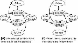

  

  Possible ways to combine and separate SS and SJ

A predicate of the form $\theta _S$ can be instantiated as a Similarity Sel. ($\theta _{S,C} (e)$) or Similarity Join ($\theta _S (e,f)$) predicate. Figure 14 graphically represents all the ways in which SS and SJ predicates can be combined. The following observations can be drawn from it:

• We consider two generic cases: when the selection predicate attribute is the outer attribute in the join predicate, and when it is the inner one. This distinction is relevant, that is, generates different equivalence rules, when the SJ operation is not commutative (kNN-Join and Join-Around). In general, if the join operation is commutative ($\varepsilon$-Join and kD-Join), the rules for both cases are the same. Commutativity of SJ operations is discussed in Sect. 4.2.1.

• Since Join-Around is a hybrid between the kNN-Join with $k$=1 and the $\varepsilon$-Join, the way this operation can be combined with a given SS operator corresponds to the most restricted way in which the kNN-Join or the $\varepsilon$-Join can be combined with that SS operator. This observation applies in fact to any rule that uses Join-Around.

• The rules where the selection attribute is the inner join attribute (Fig. 14a) are equal to or more restrictive than the corresponding rules where the selection attribute is the outer join attribute (Fig. 14b).

The instances of GR2 and GR3 are presented in “Appendix” (R5-R31). We describe several of them next. Based on GR2 (when the selection attribute is the inner join attribute), the doubly directed edge between nodes $\varepsilon$-Join and $\varepsilon$-Sel. in Fig. 14a states that these predicates can be combined/separated in any order, this is:

$$\begin{aligned} \sigma _{\theta _{\varepsilon \,1}(e1,e2)\cap \theta _{\varepsilon 2,C}(e2)}(E)&\equiv \sigma _{\theta _{\varepsilon \,1}(e1,e2)}(\sigma _{\theta _{\varepsilon 2,C}(e2)}(E))\\&\equiv \sigma _{\theta _{\varepsilon \,2,C}(e2)}(\sigma _{\theta _{\varepsilon 1}(e1,e2)}(E)). \end{aligned}$$

(R5)

Observe that the middle plan of R5 executes the $\varepsilon$-Sel. first, while the RHS plan executes the $\varepsilon$-Join first. R5 is graphically represented in Fig. 15. Also considering GR2, the directed edge from kNN-Join to $\varepsilon$-Selection in Fig. 14a represents that these predicates can be combined or separated only if the kNN-Join is executed before the $\varepsilon$-Selection, this is:

$$\begin{aligned} \sigma _{\theta _{kNN}(e1,e2)\cap \theta _{\varepsilon ,C}(e2)}(E) \not \equiv \sigma _{\theta _{kNN}(e1,e2)}(\sigma _{\theta _{\varepsilon ,C}(e2)}(E)). \end{aligned}$$

(R8)

$$\begin{aligned} \sigma _{\theta _{kNN}(e1,e2)\cap \theta _{\varepsilon ,C}(e2)}(E) \equiv \sigma _{\theta _{\varepsilon ,C}(e2)}(\sigma _{\theta _{kNN}(e1,e2)}(E)). \end{aligned}$$

(R9)

Fig. 15

Combining/separating $\varepsilon$-Join and $\varepsilon$-Sel. (R5)

The RHS plan of R8 executes $\varepsilon$-Sel. first and produces a different result than the LHS plan. This is illustrated in the bottom plan of Fig. 16. The RHS plan of R9, on the other hand, executes kNN-Join first and is equivalent to the LHS plan. This is illustrated in the top plan of the same figure. Let us consider now the same pair of nodes (kNN-Join and $\varepsilon$-Selection) under GR3 (when the selection attribute is the outer join attribute). The edge between these nodes is now a doubly directed edge (Fig. 14b) and consequently the predicates can be combined or separated in any order:

$$\begin{aligned} \sigma _{\theta _{kNN}(e1,e2)\cap \theta _{\varepsilon ,C}(e1)}(E)&\!\equiv \! \sigma _{\theta _{kNN}(e1,e2)}(\sigma _{\theta _{\varepsilon ,C}(e1)}(E))\\&\!\equiv \! \sigma _{\theta _{\varepsilon ,C}(e1)}(\sigma _{\theta _{kNN}(e1,e2)}(E)). \end{aligned}$$

(R23)

Observe that the middle plan of R23 executes the $\varepsilon$-Sel. first while the RHS plan executes the kNN-Join first. Figure 17 shows an example of R23. Finally, considering also GR3, the dotted edge between kD-Join and kNN-Selection in Fig. 14b specifies that these predicates cannot be combined or separated in any order (R27, R28).

Fig. 16

Combining/separ. kNN-Join and $\varepsilon$-Sel. (R8, R9)

Fig. 17

Combining/separating kNN-Join and $\varepsilon$-Sel. (R23)

TPC-H Example of R23: Find the closest three suppliers for every customer within 100 miles from our Chicago headquarters (X,Y). The SQL and evaluation plans based on R23 are presented below.

$\sigma _{\theta _{kNN=3}(c\_loc,s\_loc)\cap \theta _{\varepsilon =100,C=(X,Y)}(c\_loc)}(C \times S) \equiv$

$\sigma _{\theta _{kNN=3}(c\_loc,s\_loc)}(\sigma _{\theta _{\varepsilon =100,C=(X,Y)}(c\_loc)}(C \times S)) \equiv$

$\sigma _{\theta _{\varepsilon =100,C=(X,Y)}(c\_loc)}(\sigma _{\theta _{kNN=3}(c\_loc,s\_loc)}(C \times S)).$

These plans can be further transformed using additional rules. For instance, since $\sigma _{\theta _S(e,f)}(E \times F) \equiv E \bowtie _{\theta _S(e,f)} F$ (see Sect. 3.2), the last plan is equivalent to:

$\sigma _{\theta _{\varepsilon =100,C=(X,Y)}(c\_loc)}(C \bowtie _{\theta _{kNN=3}(c\_loc,s\_loc)} S).$

Proof sketch of Rule R9 kNN-Join is defined over two relations. Assume that $\theta _{kNN}$ is defined over relations $E_1$ and $E_2$, and that the input relation $E$ is the cross product of all the relations involved in the similarity-aware predicates, that is, $E = E_1 \times E_2$. Furthermore, we assume that the join attributes are $E_1.e_1$ and $E_2.e_2$. Consider a generic tuple $t_{E1}$ of $E_1$. We will show that for any possible pair ($t_{E1}$,$t_{E2}$), where $t_{E2}$ is a tuple of $E_2$, the results generated by the plans of both sides of the rule are the same. The top part of Fig. 18a gives a graphical representation of Rule R9. Using the conceptual evaluation order of similarity queries, we can transform the left part of the rule to an equivalent expression that uses the intersection operation as represented in the bottom part of Fig. 18a. We will use this version of the rule in the remaining part of the proof. Figure 18b gives the different possible regions for the value of $t_{E2}.e_2$. Note that the region marked as kNN (which comprises regions $B$ and $M$) represents the region that contains the kNN closest neighbors of $t_{E1}$ in $E_2$.

• 1. When the value of $t_{E2}.e_2$ belongs to $A$. In the LHS plan, ($t_{E1}$,$t_{E2}$) is not selected in any of the operators. No output is generated by this plan. In the RHS plan, ($t_{E1}$,$t_{E2}$) is filtered out by the bottom selection since $t_{E2}$ is not one of the kNN closest neighbors of $t_{E1}$ in $E_2$. No tuple flows to the top operator and no output is generated by this plan.

  Fig. 18

  

  Combining kNN-Join and $\varepsilon$-Sel. (R9)—proof

• 2. When the value of $t_{E2}.e_2$ belongs to $B$. In the LHS plan, the pair ($t_{E1}$,$t_{E2}$) is selected in the left operator but not in the right one. The intersection operator does not produce any output and consequently no output is generated by this plan. In the RHS plan, ($t_{E1}$,$t_{E2}$) is selected in the bottom selection since $t_{E2}$ is one of the kNN closest neighbors of $t_{E1}$ in $E_2$. However, ($t_{E1}$,$t_{E2}$) is filtered out by the top selection because $dist(t_{E2}.e_2 ,C)>\varepsilon$. Thus, no output is generated by this plan either.

• 3. When the value of $t_{E2}.e_2$ belongs to $M$. In the LHS plan, ($t_{E1}$,$t_{E2}$) is selected in both operators. Consequently, ($t_{E1}$,$t_{E2}$) belongs to the output of the intersection and the LHS plan. In the RHS plan, ($t_{E1}$,$t_{E2}$) is selected by the bottom selection since $t_{E2}$ is one of the kNN closest neighbors of $t_{E1}$ in $E_2$. ($t_{E1}$,$t_{E2}$) is also selected by the top selection since $dist(t_{E2}.e_2 ,C)\le \varepsilon$. Thus, ($t_{E1}$,$t_{E2}$) belongs also to the output of the RHS plan.

• 4. When the value of $t_{E2}.e_2$ belongs to $D$. In the LHS plan, the pair ($t_{E1}$,$t_{E2}$) is selected in the right similarity operator but not in the left one. The intersection operator does not produce any output and thus no output is generated by this plan. In the RHS plan, ($t_{E1}$,$t_{E2}$) is filtered out by the bottom selection. No tuple flows to the top operator. Thus, no output is generated by this plan either. $\square$

4.1.3 Combining/separating Similarity Join predicates

Multiple SJ predicates can be combined or separated using the following general rules.

When the attributes in the predicates have a single direction ($e1 \rightarrow e2$, $e2 \rightarrow e3$):

• GR4. $\sigma _{\theta _{S1}(e1,e2)\cap \theta _{S2}(e2,e3)}(E) \equiv \sigma _{\theta _{S1}(e1,e2)}(\sigma _{\theta _{S2}(e2,e3)} (E))$, and $\sigma _{\theta _{S1}(e1,e2)\cap \theta _{S2}(e2,e3)}(E) \equiv \sigma _{\theta _{S2}(e2,e3)} (\sigma _{\theta _{S1}(e1,e2)}$ $(E))$, if the graph of Fig. 19a has a doubly directed edge of the form: $S1\xleftarrow {(e1,e2)} \xrightarrow {(e2,e3)}S2$.

  Fig. 19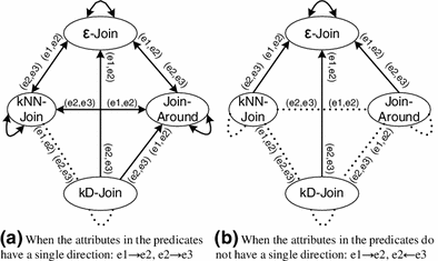

  

  Possible ways to combine/separate SJ predicates

• GR5. $\sigma _{\theta _{S1}(e1,e2)\cap \theta _{S2}(e2,e3)}(E) \equiv \sigma _{\theta _{S1}(e1,e2)}(\sigma _{\theta _{S2}(e2,e3)} (E))$, and $\sigma _{\theta _{S1}(e1,e2)\cap \theta _{S2}(e2,e3)}(E) \not \equiv \sigma _{\theta _{S2}(e2,e3)} (\sigma _{\theta _{S1}(e1,e2)}$ $(E))$, if the graph of Fig. 19a has a directed edge of the form: $S1\xleftarrow {(e1,e2) (e2,e3)}S2$.

When the attributes in the predicates do not have a single direction ($e1 \rightarrow e2$, $e2 \leftarrow e3$):

• GR6. $\sigma _{\theta _{S1}(e1,e2)\cap \theta _{S2}(e3,e2)}(E) \equiv \sigma _{\theta _{S1}(e1,e2)}(\sigma _{\theta _{S2}(e3,e2)} (E))$, and $\sigma _{\theta _{S1}(e1,e2)\cap \theta _{S2}(e3,e2)}(E) \equiv \sigma _{\theta _{S2}(e3,e2)} (\sigma _{\theta _{S1}(e1,e2)}$ $(E))$, if the graph of Fig. 19b has a doubly directed edge of the form: $S1\xleftarrow {(e1,e2)} \xrightarrow {(e3,e2)}S2$.

• GR7. $\sigma _{\theta _{S1}(e1,e2)\cap \theta _{S2}(e3,e2)}(E) \equiv \sigma _{\theta _{S1}(e1,e2)}(\sigma _{\theta _{S2}(e3,e2)} (E))$, and $\sigma _{\theta _{S1}(e1,e2)\cap \theta _{S2}(e3,e2)}(E) \not \equiv \sigma _{\theta _{S2}(e3,e2)} (\sigma _{\theta _{S1}(e1,e2)}$ $(E))$, if the graph of Fig. 19b has a directed edge of the form: $S1\xleftarrow {(e1,e2) (e3,e2)}S2$.

If the edge between two nodes is dotted in Fig. 19, none of the equivalences presented in rules GR4 or GR6 hold. The graphs in Fig. 19 show the different ways in which two SJ predicates can be combined/separated. Two cases are considered: when the attributes in the predicates have a single direction, for example, $e1 \rightarrow e2$, $e2 \rightarrow e3$; and when this is not the case, for example, $e1 \rightarrow e2$, $e2 \leftarrow e3$. In general, this classification generates different equivalence rules when at least one of the SJ operations is not commutative (kNN-Join and Join-Around). The “Appendix” presents all the instances of GR4-GR7 (R32-R65). We describe some of these here.

Under GR4 (predicates’ attributes have a single direction: $e1 \rightarrow e2$, $e2 \rightarrow e3$), the doubly directed edge that starts and ends at the $\varepsilon$-Join node in Fig. 19a specifies that two $\varepsilon$-Join predicates can be combined in any order. This is:

$$\begin{aligned} \sigma _{\theta _{\varepsilon \,1}(e1,e2)\cap \theta _{\varepsilon \,2}(e2,e3)}(E) \!\equiv \! \sigma _{\theta _{\varepsilon \,1}(e1,e2)}(\sigma _{\theta _{\varepsilon \,2}(e2,e3)}(E))\\ \!\equiv \! \sigma _{\theta _{\varepsilon \,2}(e2,e3)}(\sigma _{\theta _{\varepsilon \,1}(e1,e2)}(E)). \end{aligned}$$

(R32)

Rule R32 is presented graphically in Fig. 20.

Fig. 20

Combining/separating two $\varepsilon$-Join predicates (R32)

Under GR7 (predicates’ attributes do not have a single direction: $e1 \rightarrow e2$, $e2 \leftarrow e3$), the directed edge from kNN-Join to $\varepsilon$-Join in Fig. 19b states that these predicates can be combined executing kNN-Join first:

$$\begin{aligned} \sigma _{\theta _{\varepsilon }(e1,e2)\cap \theta _{kNN}(e3,e2)}(E) \equiv \sigma _{\theta _{\varepsilon }(e1,e2)}(\sigma _{\theta _{kNN}(e3,e2)}(E)). \end{aligned}$$

(R52)

$$\begin{aligned} \sigma _{\theta _{\varepsilon }(e1,e2)\cap \theta _{kNN}(e3,e2)}(E) \not \equiv \sigma _{\theta _{kNN}(e3,e2)}(\sigma _{\theta _{\varepsilon }(e1,e2)}(E)). \end{aligned}$$

(R53)

kNN-Join is executed first in the RHS plan of R52 while $\varepsilon$-Join is executed first in the RHS plan of R53.

4.2 Other core equivalence rules

4.2.1 Commutativity of Similarity Join operators

Some SJ operations ($\varepsilon$-Join and kD-Join) are commutative as specified by the following general rule.

• GR8. $E \bowtie _{\theta _S(e,f)} F \equiv F \bowtie _{\theta _S(e,f)} E$, when (i) $S$ is $\varepsilon$-Join or kD-Join but not kNN-Join or Join-Around, and (ii) the distance function used in the operations is symmetric.

4.2.2 Distribution of (similarity or regular) selection over (similarity or regular) join

Pushing selection below join (distributing selection over join) is one of the most useful rules in regular relational algebra. In this section, we extend this rule to the case of SS and SJ. Similarity or regular selection operations can be pushed below similarity or regular join operations according to the following general rules.

When the selection predicate attribute is the outer attribute in the join predicate:

• GR9. $\sigma _{\theta _{S1}(e)}(E\bowtie _{\theta _{S2}(e,f)}F) \equiv (\sigma _{\theta _{S1}(e)}(E))\bowtie _{\theta _{S2}(e,f)}F$, if cell [$S1$, $S2$] in Table 1a is checked.

  Table 1 Cases where selection can be pushed below join

When the selection predicate attribute is the inner attribute in the join predicate:

• GR10. $\sigma _{\theta _{S1}(f)}(E\bowtie _{\theta _{S2}(e,f)}F) \equiv E\bowtie _{\theta _{S2}(e,f)}(\sigma _{\theta _{S1}(f)}$ $(F))$, if cell [$S1$, $S2$] in Table 1b is checked.

Table 1 summarizes all the cases where a selection operator (regular or similarity-aware) can be pushed below a join (regular or similarity-aware). This table and general rules GR9 and GR10 consider two generic cases: when the selection attribute is the outer attribute of the join predicate and when it is the inner one. The instances of GR9 and GR10 (R70-R101) are included in the “Appendix”. Some of them are presented next.

In some cases, a given selection type can be pushed below either input of a join. For instance, this is the case for regular selection and $\varepsilon$-Join. Note that both cells [Regular Selection, $\varepsilon$-Join] in Table 1a and b have a check mark. Using GR9 and GR10 we obtain:

$$\begin{aligned} \sigma _{\theta (e)}(E\bowtie _{\theta _{\varepsilon }(e,f)}F) \equiv (\sigma _{\theta (e)}(E))\bowtie _{\theta _{\varepsilon }(e,f)}F. \end{aligned}$$

(R70)

$$\begin{aligned} \sigma _{\theta (f)}(E\bowtie _{\theta _{\varepsilon }(e,f)}F) \equiv E\bowtie _{\theta _{\varepsilon }(e,f)}(\sigma _{\theta (f)}(F)). \end{aligned}$$

(R71)

In R70, selection is pushed below the outer input of $\varepsilon$-Join; in R70, below the inner one. Figure 21a represents Rule R70 graphically. Similarly, for the case of $\varepsilon$-Selection and $\varepsilon$-Join we have:

$$\begin{aligned} \sigma _{\theta _{\varepsilon \,1,C}(e)}(E\bowtie _{\theta _{\varepsilon \,2}(e,f)}F) \equiv (\sigma _{\theta _{\varepsilon \,1,C}(e)}(E))\bowtie _{\theta _{\varepsilon \,2}(e,f)}F. \end{aligned}$$

(R86)

$$\begin{aligned} \sigma _{\theta _{\varepsilon \,1,C}(f)}(E\bowtie _{\theta _{\varepsilon \,2}(e,f)}F) \equiv E\bowtie _{\theta _{\varepsilon \,2}(e,f)}(\sigma _{\theta _{\varepsilon \,1,C}(f)}(F)). \end{aligned}$$

(R87)

Fig. 21

Distribution of selection over $\varepsilon$-Join (R70)

In other cases, selection can only be pushed below the outer input of a join. This is the case for $\varepsilon$-Join and kNN-Join. Note that the cell [Regular Selection, $\varepsilon$-Join] has a check mark only in Table 1a. Using GR9 and GR10, we get the following rules:

$$\begin{aligned} \sigma _{\theta _{\varepsilon ,C}(e)}(E\bowtie _{\theta _{kNN}(e,f)}F) \equiv (\sigma _{\theta _{\varepsilon ,C}(e)}(E))\bowtie _{\theta _{kNN}(e,f)}F. \end{aligned}$$

(R88)

$$\begin{aligned} \sigma _{\theta _{\varepsilon ,C}(f)}(E\bowtie _{\theta _{kNN}(e,f)}F) \not \equiv E\bowtie _{\theta _{kNN}(e,f)}(\sigma _{\theta _{\varepsilon ,C}(f)}(F)). \end{aligned}$$

(R89)

Figure 22 shows that pushing $\varepsilon$-Sel. below the outer input of kNN-Join generates the same result as executing kNN-Join first. On the other hand, pushing $\varepsilon$-Sel. below the inner input of kNN-Join can generate a different result as seen in Fig. 23.

Fig. 22

Distribution of $\varepsilon$-Sel. over kNN-Join—when sel. is pushed below the outer relation (R88)

Fig. 23

Distribution of $\varepsilon$-Sel. over kNN-Join—when sel. is pushed below the inner relation (R89)

TPC-H Example of R86: Considering the customers that are located within 200 miles from our Chicago headquarters (X,Y), identify the customers that are located within 10 miles of certain locations of interest (INTER_ LOCATION). The SQL and evaluation plans based on R86 are presented below.

$\sigma _{\theta _{\varepsilon \,1=200,C=(X,Y)}(c\_loc)}(C\bowtie _{\theta _{\varepsilon \,2=10}(c\_loc,il\_loc)}IL) \equiv$

$(\sigma _{\theta _{\varepsilon \,1=200,C=(X,Y)}(c\_loc)}(C))\bowtie _{\theta _{\varepsilon \,2=10}(c\_loc,il\_loc)}IL.$

Proof sketch of Rule R70 The join attributes in $\theta _\varepsilon$ are $E.e$ and $F.f$, and $\theta$ is defined over $E.e$. Consider a generic tuple $t_E$ of $E$. We will show that for any possible pair ($t_E$,$t_F$), where $t_F$ is a tuple of $F$, the results generated by the plans of both sides of the rule are the same. Figure 21b gives the different possible regions for the values of $t_F.f$, and two generic values of $t_E.e$. $a_2$ represent a value that satisfies the predicate $\theta$ while $a_1$ represents a value that does not.

• 1. When the value of $t_E.e$ is $a_1$. In the LHS plan, the pair ($t_E$,$t_F$) may or may not belong to the output of the $\varepsilon$-Join. However, ($t_E$,$t_F$) will be filtered out by the selection operator since $a_1$ does not satisfy the predicate $\theta$. Thus, no output is generated by this plan. In the RHS plan, $t_E$ is filtered out by the selection since $a_1$ does not satisfy $\theta$. No tuple flows to the $\varepsilon$-Join operator from its outer input. Thus, no output is generated by this plan either.

• 2. When the value of $t_E.e$ is $a_2$ and the value of $t_F.f$ belongs to $A$. In the LHS plan, the pair ($t_E$,$t_F$) does not belong to the output of the $\varepsilon$-Join since $dist(t_E.e,t_F.f)>\varepsilon$. No tuple flows to the selection operator. Thus, no output is generated by this plan. In the RHS plan, $t_E$ is selected by the regular selection operator since $a_2$ satisfies $\theta$. However, the pair ($t_E$,$t_F$) does not belong to the output of the $\varepsilon$-Join since $dist(t_E.e,t_F.f)>\varepsilon$. Thus, no output is generated by this plan either.

• 3. When $t_E.e$ is $a_2$ and the value of $t_F.f$ belongs to $B$. In the LHS plan, the pair ($t_E$,$t_F$) belongs to the output of the $\varepsilon$-Join since $dist(t_E.e,t_F.f) \le \varepsilon$. ($t_E$,$t_F$) is also selected by the regular operator since $a_2$ satisfies $\theta$. ($t_E$,$t_F$) belongs to the output of this plan. In the RHS plan, $t_E$ is selected by the selection operator since $a_2$ satisfies $\theta$. ($t_E$,$t_F$) belongs to the output of the $\varepsilon$-Join since $dist(t_E.e,t_F.f) \le \varepsilon$. Thus, ($t_E$,$t_F$) also belongs to the output of this plan.$\square$

4.2.3 Associativity of Similarity Join operators

Associativity of join operators is another core transformation rule commonly used in query optimization. This rule allows re-ordering multiple join operations and can significantly improve the efficiency of a query because different orders can generate different sizes of the intermediate results. In general, plans with smaller intermediate results are also more efficient. SJ operations are associative according to the following general rules.

When the attributes in the predicates have a single direction ($e \rightarrow f$, $f \rightarrow g$):

• GR11. $(E\bowtie _{\theta _{S1}(e,f)}F)\bowtie _{\theta _{S2}(f,g)}G \equiv E \bowtie _{\theta _{S1}(e,f)} (F\bowtie _{\theta _{S2}(f,g)}G)$, when $S1$ and $S2$ are both: $\varepsilon$-Join, kNN-Join, or Join-Around but not kD-Join.

When the predicates’ attributes do not have a single direction ($e \rightarrow f$, $f \leftarrow g$):

• GR12. $G \bowtie _{\theta _{S1}(g,f)}(E\bowtie _{\theta _{S2}(e,f)}F) \equiv E \bowtie _{\theta _{S2}(e,f)}(G\bowtie _{\theta _{S1}(g,f)}F)$, when $S1$ and $S2$ are both: $\varepsilon$-Join but not kNN-Join, kD-Join or Join-Around.

The associativity of multiple SJ operators depends in general on whether or not the predicates’ attributes have a single direction. This distinction, however, is not relevant (generate the same rules) when the join operators are commutative ($\varepsilon$-Join and kD-Join). All the instances of GR11 and GR12 are presented in the “Appendix” (R102 to R109). We describe here some of them.

In the case of a query with two $\varepsilon$-Join operations, based on GR11 and GR12, we can re-order the operations whether the attributes in the predicates have a single direction or not. The corresponding rule instances are:

$$\begin{aligned}&(E\bowtie _{\theta _{\varepsilon \,1}(e,f)}F)\bowtie _{\theta _{\varepsilon \,2}(f,g)}G \equiv \\&E \bowtie _{\theta _{\varepsilon \,1}(e,f)}(F\bowtie _{\theta _{\varepsilon \,2}(f,g)}G). \end{aligned}$$

(R102)

$$\begin{aligned}&G \bowtie _{\theta _{\varepsilon \,1}(g,f)}(E\bowtie _{\theta _{\varepsilon \,2}(e,f)}F) \equiv \\&E \bowtie _{\theta _{\varepsilon \,2}(e,f)}(G\bowtie _{\theta _{\varepsilon \,1}(g,f)}F). \end{aligned}$$

(R106)

The left and right plans of Fig. 24 represent the LHS and LHS plans of R102, respectively. The left plan in the figure performs first the join on $e$ and $f$ and then the one on $f$ and $g$. The right plan performs first the join on $f$ and $g$ and then the one on $e$ and $f$.

Fig. 24

Associativity of $\varepsilon$-Join operators (R102)

GR11 and GR12 also specify that kNN-Join operations are associative only when the attributes in the predicates have a single direction. This is:

$$\begin{aligned} (E\bowtie _{\theta _{kNN1}(e,f)}F)\bowtie _{\theta _{kNN2}(f,g)}G \equiv \\ E \bowtie _{\theta _{kNN1}(e,f)}(F\bowtie _{\theta _{kNN2}(f,g)}G). \end{aligned}$$

(R103)

$$\begin{aligned} G \bowtie _{\theta _{kNN1}(g,f)}(E\bowtie _{\theta _{kNN2}(e,f)}F) \not \equiv \\ E \bowtie _{\theta _{kNN2}(e,f)}(G\bowtie _{\theta _{kNN1}(g,f)}F). \end{aligned}$$

(R107)

Figure 25 shows an example of associativity of kNN-Join operations (R103, single direction). Figure 26 shows an example where two kNN-Join operations are not associative (R107, not single direction).

Fig. 25

Associativity of kNN-Join—when the attributes in the predicates have a single direction: $e \rightarrow f$, $f \rightarrow g$ (R103)

Fig. 26

Associativity of kNN-Join—when the attributes do not have a single direction: $e \rightarrow f$, $f \leftarrow g$ (R107)

TPC-H Example of R103: For every customer, identify its closest 3 suppliers, and for each such supplier, identify its closest 2 potential new suppliers (POT_SUP-PLIER). The SQL and evaluation plans based on R103 are presented below.

$(C\bowtie _{\theta _{kNN1=3}(c\_loc,s\_loc)}S)\bowtie _{\theta _{kNN2=2}(s\_loc,psu\_loc)}PSU \equiv$

$C \bowtie _{\theta _{kNN1=3}(c\_loc,s\_loc)}(S\bowtie _{\theta _{kNN2=2}(s\_loc,psu\_loc)}PSU).$

4.2.4 Other conventional equivalence rules

We briefly discuss here the extension of less common rules to the case of similarity operators. Selection and Similarity Selection on grouping attributes cannot be pushed below any type of SGB. $\varepsilon$-Selection distributes over set operations in the same way regular selection does, kNN-Selection does not distribute over any set operation. Finally, projection distributes over SJ operations in the same way it does over non-similarity joins. Details of these rules are included in [25].

4.3 Rules that take advantage of distance function properties

4.3.1 Pushing a selection predicate to an originally unrelated $\varepsilon$-Join operand

In the rules of Sect. 4.2.2, each selection predicate $\theta$ is pushed only to the join operand that contains the attribute referenced in $\theta$. In the case of $\varepsilon$-Join, the filtering benefits of pushing selection below join can be extended by pushing $\theta$ or a variant of it to both $\varepsilon$-Join operands as shown in the following rule (Fig. 27).

• GR13. $\sigma _{\theta (e)}(E\bowtie _{\theta _\varepsilon (e,f)}F) \equiv (\sigma _{\theta (e)}(E)) \bowtie _{\theta _\varepsilon (e,f)}$ $(\sigma _{\theta \pm \varepsilon (f)}(F)).$

  Fig. 27

  

  Pushing selection predicate to an originally unrelated $\varepsilon$-Join operand (GR13)

In this rule, (i) the distance function should satisfy the properties: Triangular Inequality, Symmetry, and Identity of Indiscernibles; and (ii) the selection predicate $\theta \pm \varepsilon (f)$ represents a modified version of $\theta$ where each condition is extended by $\varepsilon$. $\theta \pm \varepsilon (f)$ is applied on $f$, the join attribute in $F$, and uses the same distance function used in $\theta$. For example, if $\theta (e)$ is $10 \le e \le 20$, then $\theta \pm \varepsilon (f)$ is $10-\varepsilon \le f \le 20+\varepsilon$.

TPC-H Example of GR13: For every balance level of interest B (BAL_LEVELS), identify the customers with account balances within 500 of B. Consider only customers with balances between 2,000 and 50,000. The SQL and evaluation plans based on GR13 are presented below. In this case, $\theta (c\_acctbal)$ is $2{,}000 \le c\_acctbal \le 50{,}000$ and $\theta \pm \varepsilon (bl\_bal)$ is $1{,}500 \le bl\_bal \le 50{,}500$.

$\sigma _{\theta (c\_acctbal)}(C\bowtie _{\theta _{\varepsilon =500}(c\_acctbal,bl\_bal)}BL) \equiv$

$(\sigma _{\theta (c\_acctbal)}(C)) \bowtie _{\theta _{\varepsilon =500}(c\_acctbal,bl\_bal)}$

$(\sigma _{\theta \pm \varepsilon (bl\_bal)} (BL)).$

Proof sketch of Rule GR13 Pushing selection to the outer input of $\varepsilon$-Join was studied in R70. We focus here on the validity of pushing selection to the inner input of the $\varepsilon$-Join. Assume that in the LHS part of Rule GR13, the selection predicate $\theta (e)$ is $e=C$ and the $\varepsilon$-Join predicate $\theta _\varepsilon (e,f)$ is $dist(e,f) \le \varepsilon$.

• 1. Since $dist$ satisfies Identity of Indiscernibles, we know that $dist(e,C) = 0$.

• 2. $dist$ also satisfies the Triangular Inequality property, thus $dist(C,f) \le dist(C,e)+ dist(e,f)$.

• 3. Due to Commutativity, we have that $dist(C,f) \le dist(e,C) + dist(e,f)$.

• 4. Replacing (1) in (3), $dist(C,f) \le 0+dist(e,f) \le dist(e,f)$.

• 5. Using in (4) the fact that $dist(e,f) \le \varepsilon$, $dist(C,f) \le \varepsilon$.

The expression in (5) $dist(C,f) \le \varepsilon$ represents the selection predicate being applied on $f$ in the inner input of the RHS part of Rule GR13. We could extend this analysis to other types of selection conditions.$\square$

4.3.2 Pushing an $\varepsilon$-selection predicate to an originally unrelated $\varepsilon$-Join operand

The rules of Sect. 4.2.2 allow pushing an SS predicate $\theta _S$ to the SJ operand that contains the attribute used in $\theta _S$. In the case of $\varepsilon$-Join and $\varepsilon$-Selection, we can further reduce the size of the intermediate results by pushing $\theta _S$ to one join operand and a variant of $\theta _S$ to the other one as shown in the following equivalence rule (Fig. 28).

• GR14. $\sigma _{\theta _{\varepsilon \,1,C}(e)}(E\bowtie _{\theta _{\varepsilon \,2}(e,f)}F) \equiv (\sigma _{\theta _{\varepsilon \,1,C}(e)}(E)) \bowtie _{\theta _{\varepsilon \,2}(e,f)}(\sigma _{\theta _{(\varepsilon \,1 + \varepsilon \,2),C}(f)}(F)).$

  Fig. 28

  

  Pushing $\varepsilon$-Selection predicate to an originally unrelated $\varepsilon$-Join operand (GR14)

In this rule, (i) all $\varepsilon$-Selection and $\varepsilon$-Join operators use the same distance function; (ii) the distance function should satisfy the Triangular Inequality and Symmetry properties; and (iii) the selection predicate $\theta _{(\varepsilon \,1 + \varepsilon \,2),C}$ represents an $\varepsilon$-Selection predicate with a value of $\varepsilon$ equal to $\varepsilon \,1 + \varepsilon \,2$, where $\varepsilon \,1$ and $\varepsilon \,2$ are the values of epsilon used in the $\varepsilon$-Selection and $\varepsilon$-Join operators, respectively. For example, if $\theta _{\varepsilon \,1,C}(e)$ is $dist(e,C) \le 10$, and $\theta _{\varepsilon \,2}(e,f)$ is $dist(e,f) \le 5$, then $\theta _{(\varepsilon \,1 + \varepsilon \,2),C}(f)$ is $dist(f,C) \le 15$.

4.3.3 Associativity rule that enables joining on originally unrelated attributes

In the associativity rules described in Sect. 4.2.3, each SJ predicate involves the same attributes in both sides of the rules. In the case of $\varepsilon$-Join, when the attributes $e$ of $E$ and $f$ of $F$ are joined using $\varepsilon$1 and the result joined with attribute $g$ of $G$ using $\varepsilon$2, there is an implicit relationship between $e$ and $g$ that can be used to generate a potentially more efficient plan as shown in the following equivalence rule.

• GR15. $(E\bowtie _{\theta _{\varepsilon \,1}(e,f)}F) \bowtie _{\theta _{\varepsilon \,2}(f,g)} G \equiv (E\bowtie _{\theta _{\varepsilon \,1+\varepsilon \,2}(e,g)}G) \bowtie _{\theta _{\varepsilon \,1}(e,f) \wedge \theta _{\varepsilon \,2}(f,g)} F.$

In Rule GR15, (i) all the $\varepsilon$-Join operators use the same distance function; (ii) the distance function should satisfy the Triangular Inequality and Symmetry properties; and (iii) the predicate $\theta _{\varepsilon \,1+\varepsilon \,2}(e,g)$ represents an $\varepsilon$-Join predicate with a value of $\varepsilon$ equal to $\varepsilon \,1+\varepsilon \,2$. For example, if $\theta _{\varepsilon \,1}(e,f)$ is $dist(e,f) \le 10$, and $\theta _{\varepsilon \,2}(f,g)$ is $dist(f,g) \le 5$, then $\theta _{\varepsilon \,1+\varepsilon \,2}(e,g)$ is $dist(e,g) \le 15$.

GR13-GR15 can be used with important distance functions, for example, p-norm distance, Edit distance (equal weights), Hamming distance, and Jaccard distance.

4.4 Eager and Lazy transformations with SJ and SGB

Another important query optimization approach is the use of pull-up and push-down techniques to move the grouping operator up and down the query tree. These techniques were proposed for regular (non-similarity) operators by Chaudhuri et al. [26] and Yan et al. [27]. The main Eager and Lazy aggregations theorem [27] enables several pull-up and push-down techniques for the regular join and group-by operators. This theorem allows the pre-aggregation of data before the join operator to reduce its input size. This subsection presents the extension of the main theorem to the case of SJ and SGB. Figures 29, 30, 31 illustrate several cases of the Eager and Lazy transformations that are studied in detail in this section. In general, the single aggregation operator of the Lazy approach is split into two parts in the Eager approach. The first part pre-evaluates some aggregation functions and calculates the count before the join. The second part uses the intermediate information to calculate the final results after the join. Both the Eager and Lazy plans should be considered during query optimization since neither of them is the best approach in all scenarios. The notation used in this section, given in Table 2, allows a direct comparison with analogous theorems for regular operators and uses a convenient representation of the operators’ arguments that facilitates the presentation of theorems and proofs. The proofs of the presented theorems are included in [25].

Fig. 29

Eager/lazy aggregation with SGB and join

Fig. 30

Eager/Lazy aggregation with group-by and SJ

Fig. 31

Eager/Lazy aggregation with SGB and SJ

Table 2 Notation for eager/lazy transformation theorems

4.4.1 Eager and Lazy transformations with SGB and join

Eager and Lazy transformations can be extended to the case of SGB and regular join as shown in Theorem 1.

Theorem 1

(Eager/Lazy Aggregation Main Theorem for SGB and Join) The following two expressions:

• E1. $F[AA_d, AA_u]$ $_A[GA_d$, $GA_u, AA_d, AA_u] g[GA_d,$ $GA_u;$Seg$]\sigma [C_d \wedge C_u](R_d \bowtie _{C0} R_u)$,

• E2. $_D[GA_d, GA_u,$FAA$](F_{ua}[AA_u,$CNT$], F_{d2}[$FAA$_d])$ $_A[GA_d, GA_u, AA_u,$FAA$_d,$CNT$] g [GA_d, GA_u;$Seg$_u]$ $\sigma [C_u](((F_{d1}[AA_d],$COUNT$)$ $_A[$NGA$_d, {GA_d}^+, AA_d]$ $g[$NGA$_d;$Seg$_d] \sigma [C_d]R_d) \bowtie _{C0} R_u)$,

are equivalent if (i) $F_d$ can be decomposed into $F_{d1}$ and $F_{d2}$, (ii) $F_u$ contains only class $C$ or $D$ aggregation functions [27], (iii) NGA$_d \rightarrow {GA_d}^+$ holds in $\sigma [C_d]R_d$, and (iv) $\alpha (C0) \cap GA_d = \emptyset$. Expressions $E_1$ and $E_2$ represent the Lazy and Eager approaches, respectively.

Figure 29 presents an example of the application of Theorem 1. This figure gives the number of tuples that flow to and from each operator. The join in the Lazy aggregation plan processes a total of 7 tuples while the SGB node processes 5 tuples. In the Eager aggregation plan, all the tuples of $T1$ get combined into one tuple in the bottom SGB node, and the join and top SGB only need to process 3 and 1 tuples, respectively.

TPC-H Example of Theorem 1: Cluster all the order discounts around a set of discount levels of interest (DCNT _LEVELS) and for each cluster report the sum of discounts given by each clerk type. SQL queries representing the Lazy and Eager plans are included below.

4.4.2 Eager and Lazy transformations with group-by and SJ

Eager and Lazy aggregation transformations can be extended to the case of SJ and group-by (Theorem 2).

Theorem 2

(Eager/Lazy Aggregation Main Theorem for Group-by and SJ) The following two expressions:

• E1. $F[AA_d, AA_u]$ $_A[GA_d, GA_u, AA_d, AA_u] g[GA_d,$ $GA_u]\sigma [C_d \wedge C_u](R_d \widetilde{\bowtie }_{C0} R_u)$,

• E2. $_D[GA_d, GA_u,$FAA$](F_{ua}[AA_u,$CNT$], F_{d2}[$FAA$_d])$ $\pi$ $_A[GA_d, GA_u, AA_u,$FAA$_d,$CNT$] g [GA_d, GA_u]\sigma [C_u]$ $(((F_{d1}[AA_d],$COUNT$)$ $_A[$NGA$_d, {GA_d}^+, AA_d]$ $g[$NGA$_d] \sigma [C_d]R_d) \widetilde{\bowtie }_{C0} R_u)$,

where $\widetilde{\bowtie }_{C0}$ is kNN-Join, $\varepsilon$-Join, or Join-Around, are equivalent under the same conditions as in Theorem 1.

Figure 30 illustrates Theorem 2. The SJ of the Lazy aggregation plan processes a total of 7 tuples while the grouping node processes 5 tuples. In the Eager plan, all the tuples of $T1$ get grouped into one tuple in the bottom group-by node, and the SJ and top grouping operators only need to process 3 and 1 tuples respectively. In scenarios where $T1$ has a significant number of tuples with the same value of ($G1$, $J1$), the optimizer will probably select the Eager plan.

4.4.3 Eager and Lazy transformations with SGB and SJ

The Eager and Lazy Aggregation transformations can be extended to the case of SJ and SGB as shown in the next theorem.

Theorem 3

(Eager/Lazy Aggregation Main Theorem for SGB and SJ) The following two expressions:

• E1. $F[AA_d, AA_u]$ $_A[GA_d, GA_u, AA_d, AA_u] g[GA_d,$ $GA_u;$Seg$]\sigma [C_d \wedge C_u](R_d \widetilde{\bowtie }_{C0} R_u)$,

• E2. $_D[GA_d, GA_u,$FAA$](F_{ua}[AA_u,$CNT$], F_{d2}[$FAA$_d])$ $_A$ $[GA_d, GA_u, AA_u,$FAA$_d,$CNT$] g [GA_d, GA_u;$Seg$_u]$ $\sigma [C_u](((F_{d1}[AA_d],$COUNT$)$ $_A[$NGA$_d, {GA_d}^+, AA_d]$ $g[$NGA$_d;$Seg$_d] \sigma [C_d]R_d) \widetilde{\bowtie }_{C0} R_u)$,

where $\widetilde{\bowtie }_{C0}$ is kNN-Join, $\varepsilon$-Join, or Join-Around, are equivalent under the same conditions as in Theorem 1.

An example of the use of this theorem is presented in Fig. 31. The numbers of tuples flowing in the pipelines are similar to the ones of Fig. 30. Note that the bottom grouping node of the Eager approach merges tuples that have: (i) the same value of $J1$ and (ii) values of $G2$ that belong to the same similarity group. In this example, all the tuples of $T1$ are merged even though they have different values of $G1$.

4.5 Examples of the use of transformation rules

The equivalence rules presented earlier in this section can be used to transform the conceptual evaluation plan of a similarity query into more efficient equivalent plans. This section presents examples of this type of query transformations.

Example 1

Figure 32 gives the SQL version of a similarity query with $\varepsilon$-Selection and $\varepsilon$-Join predicates. The left plan in this figure gives the conceptual evaluation plan of this query. The right plan shows an equivalent plan with potentially better execution time (since each relation is read only once and the Similarity Selection is pushed below the Similarity Join). The following steps show how the query expression of the left plan can be transformed into the one of the right plan.

• 1. $\sigma _{\theta _{\varepsilon \,1}(e,f)\cap \theta _{\varepsilon \,2,C}(e)}(E \times F)$.

  Fig. 32

  

  Query with $\varepsilon$-Selection and $\varepsilon$-Join predicates

• 2. $\equiv \sigma _{\theta _{\varepsilon \,1}(e,f)}(\sigma _{\theta _{\varepsilon \,2,C}(e)}(E \times F))$, applying Rule R20.

• 3. $\equiv \sigma _{\theta _{\varepsilon \,1}(e,f)}((\sigma _{\theta _{\varepsilon \,2,C}(e)}E) \times F)$, applying Rule R82.

• 4. $\equiv (\sigma _{\theta _{\varepsilon \,2,C}(e)}E)\bowtie _{\theta _{\varepsilon \,1}(e,f)}F$, applying Rule R110.

Example 2

Figure 33 gives the SQL expression of a similarity query with two $\varepsilon$-Join predicates. The left plan is the conceptual evaluation plan of the query while the right one is an equivalent plan with potentially better execution time (each relation is read only once and only the tuples that satisfy the bottom SJ flow to the top SJ). The following steps show the transformation of the left plan into the right one.

• 1. $\sigma _{\theta _{\varepsilon \,1}(e,f)\cap \theta _{\varepsilon \,2}(f,g)}((E \times F)\times G)$.

  Fig. 33

  

  Query with multiple $\varepsilon$-Join predicates

• 2. $\sigma _{\theta _{\varepsilon \,2}(f,g)}(\sigma _{\theta _{\varepsilon \,1}(e,f)} ((E \times F)\times G))$, applying Rule R32.

• 3. $\sigma _{\theta _{\varepsilon \,2}(f,g)} ((\sigma _{\theta _{\varepsilon \,1}(e,f)} (E \times F)) \times G )$, applying Rule R82.

• 4. $\sigma _{\theta _{\varepsilon \,2}(f,g)}((E \bowtie _{\theta _{\varepsilon \,1}(e,f)} F) \times G)$, applying Rule R110.

• 5. $(E \bowtie _{\theta _{\varepsilon \,1}(e,f)} F) \bowtie _{\theta _{\varepsilon \,2}(f,g)}G$, applying Rule R110.

Figures 34, 35, 36, 37 give examples of more complex similarity query transformations. These examples also show several key general transformation guidelines for similarity query optimization.

Fig. 34

Query with multiple sim. selection predicates

Fig. 35

Query with multiple $\varepsilon$-Join and sim. sel. predicates

Fig. 36

Query with kNN-Join and sim. sel. predicates

Fig. 37

Query with multiple sim. join and sel. predicates

Example 3

Figure 34 gives the transformation of a query with multiple Similarity Selection predicates. This figure illustrates that multiple $\varepsilon$-Selection operators over the same attribute can be serialized. Multiple kNN-Selection operators cannot be serialized; they need to be executed independently and their results combined using the intersection operator. $\varepsilon$-Selection and kNN-Selection operations over the same attribute can be serialized executing the kNN-Selection operations first.

Example 4

Figure 35 gives the transformation of a query with multiple $\varepsilon$-Join and SS predicates. This figure illustrates that $\varepsilon$-Selection and kNN-Selection can be serialized with $\varepsilon$-Join executing the SS first. Multiple $\varepsilon$-Join operations can also be serialized, that is, the results of a join are sent to the next one.

Example 5

Figure 36 gives the transformation of a query with a kNN-Join and multiple SS predicates. This figure illustrates that $\varepsilon$-Selection and kNN-Selection can be serialized with the kNN-Join executing the SS first when they are defined over the outer join attribute. $\varepsilon$-Selection defined over the inner join attribute of a kNN-Join can be serialized with the join operation executing the kNN-Join first. kNN-Selection defined over the inner join attribute of a kNN-Join cannot be serialized with the join operation. In this case, the kNN-Join and kNN-Selection operations need to be evaluated independently and the results combined using the intersection operation.

Example 6

Figure 37 gives the transformation of a generic query with multiple Similarity Join and Similarity Selection predicates. This figure illustrates that multiple kNN-Join operations can be serialized as long as the attributes of the join predicates have a single direction. kNN-Join and $\varepsilon$-Join can also be serialized executing the kNN-Joins first. Multiple kNN-Join operations whose predicates do not have a single direction need to be evaluated independently and the results combined using the intersection operation.

4.6 Integration of rules into query optimizers

Several elements need to be considered to fully integrate the proposed equivalence rules query optimizers.

Adding Rules to the Enumeration Framework Query optimizers generate (enumerate) equivalent plans of a query and select the one with the lowest estimated cost. Common cost-based optimizers, for instance, systems based on the Cascades [28] and Volcano [29] frameworks, combine two steps: logical exploration and physical optimization. Logical exploration applies transformation rules to generate logically equivalent plans. Since the transformation rules for similarity operators are extensions of similar rules for regular database operators, they can be integrated into query optimizers in a similar way to their non-similarity counterparts [27–29]. For instance, to create an optimizer using the Cascades framework, the associativity rule for $\varepsilon$-Join can be integrated as a rule object similar to the one for the associativity rule of regular join [28]. The physical optimization step transforms the logical operators, for example, $\varepsilon$-Join, to physical operators associated with specific implementation algorithms, for example, $\varepsilon$-Join can be implemented using the plane sweep approach (Sect. 5.2) or the QuickJoin algorithm [11].

Cost Estimation The cost of a query plan is usually computed based on the cost of individual physical operators. Both CPU and I/O costs are commonly considered. The cost of an operator depends on its implementation algorithm and on properties of its input data, for example, cardinality. The costs of the SGB and SJ implementations described in Sect. 5 are discussed in [1, 2]. Cost estimation of similarity operators, particularly of range and kNN queries using index-based access methods, has also been studied in [23, 30].

Derivation of statistics Since the cost of each operator depends on properties of its input data such as number of tuples, frequency of values, etc., it is important to have formulas to propagate these properties at every operator node. The derivation of the number of tuples for the SGB and SJ operators is discussed in [1, 2]. The number of groups of SGB-A and SGB-D can be estimated as the number of tuples of the reference objects query. The number of groups of SGB-U can be estimated as a fraction of the number of different values of the grouping attribute. In the case of Join-Around, the number of resulting tuples can be estimated as the number of tuples in the inner input dataset. In the case of $\varepsilon$-Join, more complex techniques, for example, employing histograms of the density of elements in metric spaces [23] and using a sampling based algorithm that uses Locality Sensitive Hashing [31], can be employed. The number of output tuples of the kNN-Join can be estimated as $(num\_tuples\_outer) \times min(k, num\_tuples\_inner)$ while the one of the kD-Join can be estimated as $min(num\_$ $tuples\_outer \times num\_tuples\_inner, k)$.

5 Implementing Similarity Operators

This section presents the main guidelines to implement physical similarity operators in standard DBMSs. While the definition of similarity operators, conceptual evaluation, and transformation rules presented in previous sections are applicable in general to any data type, the implementation described in this section focuses on similarity operators for numerical data. The presented implementation fulfills two key goals: (i) showing that similarity database operators can be efficiently realized and, more importantly, (ii) enabling the evaluation of transformation rules for similarity queries. The implementation of similarity operators for other data types is a task for future work. While the presentation is intended to be applicable to any DBMS, some details refer to our implementation in PostgreSQL [1, 2].

5.1 Implementing similarity Group-by operators

This subsection describes the implementation of SGB instances as physical database operators. We present the main changes at each stage of the query engine. Additional details appear in [1].

The Parser The raw-parsing grammar rules, for instance, the yacc rules in the case of PostgreSQL, are extended to recognize the SQL syntax of the SGB instances. The parse-tree and query-tree data structures are extended to include information about the type and parameters of the similarity grouping operations.

The Planner The regular aggregation node is extended to support SGB. Each extended aggregation node is able to process one similarity grouping attribute (SGA) and any number of regular grouping attributes. Figure 38a gives the structure of a plan tree with two SGAs $a1$ and $a2$. Sort nodes are added on top of the data input plan trees and the reference-points input plan trees. This order is assumed by the routines that form the similarity groups. When multiple SGAs are used, they are processed one at a time. In Fig. 38a, the bottom aggregation node applies similarity grouping on $a1$ and regular aggregation on $a2$, the result is further aggregated by the top aggregation node that applies similarity grouping on $a2$ and regular aggregation on $a1$.

Fig. 38

Path/Plan trees with SGB and SJ operators

The Executor The executor routine for the SGB operators uses a single plane sweep approach to form the groups. The tuples to be grouped and the reference points have been previously sorted and are processed simultaneously using a hash table to maintain information of the formed groups. At any time, a set of current groups is maintained, and each time the sweeping plane reaches a tuple, the system evaluates whether this tuple belongs to one of the current groups, does not belong to any group, or starts a new set of groups.

5.2 Implementing Similarity Join operators

This subsection presents the main guidelines to implement two SJ operators, $\varepsilon$-Join and Join-Around, as first-class database operators. Further details are presented in [2]. One of the goals of the implementation is to reuse and extend already available routines and structures to minimize the effort needed to realize these operators. The $\varepsilon$-Join and Join-Around operators are implemented as extensions to the Sort Merge Join (SMJ) operator and consider the case of multiple SJ predicates over numeric data.

The Parser The raw-parsing grammar rules are extended to recognize the syntax of the SJ predicates. The parse-tree and query-tree data structures are extended to include the type and parameters, for example, $\varepsilon$ and MD, of SJ predicates. The routines that transform the parse tree into the query tree are updated accordingly to process the new parse tree fields.

The Planner Figure 38b gives the structure of the plan tree generated when two SJ predicates, a $\sim$ b and c $\sim$ d, are specified. Given that the implementation is based on Sorted Merge Join, sort nodes that order by the SJ attributes are added on top of the input plan trees. This order is assumed by the routines that find the similarity matches (links). When multiple SJ predicates are specified, each predicate is processed by one SJ plan node. The results of each node are pipelined to the next node.

The Executor $\varepsilon$-Join and Join-Around are implemented extending the routines that support the Sort Merge Join operator. This allows a fast and efficient implementation of both SJ operators. The sorted tuples received from the input plans are processed synchronously following a plane sweep approach. The algorithms are coded in PostgreSQL in the fashion of a state machine. Both $\varepsilon$-Join and Join-Around use the same set of states employed by the Sorted Merge Join. The main changes to implement the SJ operators are on the routine that evaluates if there is a match between two tuples and on the way the inner cursor is restored to a previous tuple to ensure the correct generation of SJ links.

6 Performance evaluation

This section presents the performance evaluation of the implemented similarity-aware operators as well as the evaluation of the effectiveness of several transformation rules. The dataset used in the tests is based on the one specified by the TPC-H benchmark [24]. The tables of reference points and queries used in the tests are presented in Table 3. The default dataset scale factor (SF) is 5 (5GB). We use an extension of PostgreSQL that supports SGB and SJ implemented as described in Sect. 5. All the experiments are performed on an Intel Dual Core 1.83GHz machine (2GB RAM, Linux).

Table 3 Test reference points and queries

6.1 Performance evaluation of SGB

Figure 39 gives the execution time of several aggregation queries for different dataset sizes. The key result is that the execution times of all the queries that use Similarity Group-by (SGB-X) are very close to the execution time of the regular aggregation query GB. Even in the worst-case scenario represented by GB(SGB)_X, that is, queries that use SGB to produce the same result as the regular group-by, the execution time of GB(SGB) is at most only 25 % bigger than that of GB. Although, in general, it is not possible to produce the output of SGB queries using only regular SQL operations, this is feasible in some special cases, for example, SGB-A without additional clauses. Figure 40 compares the execution time of SGB-A with that of SGB(GB), a query that generates the same output as SGB-A while using only regular operators. The presented results show that the execution time and scalability properties of the SGB query are much better than those of the query that uses only regular SQL operators. The execution time of SGB(GB) grows from being 500 % bigger than that of SGB-A for SF=1 to being 1,300 % bigger for SF=14.

Fig. 39

Performance of SGB while increasing dataset size

Fig. 40

Generating similarity groups with group-by versus SGB

6.2 Performance evaluation of SJ

Figure 41 gives the execution time of the SJ-JoinAround query compared to the one of the RegOps-JoinAround query that produces the same output using only regular operators. The execution time of RegOps-JoinAround grows from being about 20 times bigger than that of SJ-JoinAround for SF=1 to being about 200 times bigger for SF=8. The poor performance of RegOps-JoinAround is due to a double nested loop join in its execution plan in addition to the use of an aggregation operation. The Join-Around operator sorts each set once and processes both sets synchronously.

Fig. 41

Perf. of Join-Around while increasing dataset size

Figure 42 gives the execution time of the SJ-EpsJoin query compared to the one of the RegOps-EpsJoin query that produces the same output using non-similarity operators. The results are presented for various values of $\varepsilon$. The value of $\varepsilon$ is a fraction of the domain range (0–11,000). This experiment uses SF=1. The key result of this experiment is that the SJ-EpsJoin query performs significantly better than the RegOps-EpsJoin query for the important case of small values of $\varepsilon$. For instance, when $\varepsilon$=1, the execution time of RegOps-EpsJoin is 4.32 s. while the one of SJ-EpsJoin is 0.96 s. The advantage of the $\varepsilon$-Join over the regular query gets reduced as the value of $\varepsilon$ increases. The performance of SJ-EpsJoin is better for small values of $\varepsilon$ because it generates shorter restorations of the inner cursor. On the other hand, RegOps-EpsJoin calculates the distance between all the combinations of outer and inner tuples.

Fig. 42

Performance of $\varepsilon$-Join while increasing $\varepsilon$

6.3 Effectiveness of transformation rules

This section demonstrates experimentally that the use of the equivalence rules for similarity queries can produce better performing plans. Even though we evaluate a subset of the rules, similar results can be obtained for the other presented rules. Like in regular relational algebra rules, the effectiveness of rules for similarity operators depends on the data. The results presented in this section should be seen as examples of what can be achieved using the proposed rules. The transformation rules for similarity operators are a core contribution of this paper. While the tests in this section use numerical data, the proposed rules could be used with operators that support in general any data type.

Effectiveness of the Associativity Transformation AssocRule_LHS and AssocRule_RHS in Fig. 43 represent the query AssocRule executed using plans that correspond to the LHS and RHS of Rule R102, respectively. The execution time of AssocRule_RHS is 9.2% of that of AssocRule_LHS. AssocRule_LHS joins ($\varepsilon$-Join) first Customer (C) and R2 generating 17,241,601 intermediate rows. The execution time of AssocRule_RHS is much smaller because it joins the two smaller tables (R1 and R2) first generating 2,519 intermediate rows.

Fig. 43

Effectiveness of the associativity transformation

Effectiveness of Pushing Selection below SJ PushSel_ LHS, PushSel_RHS1, and PushSel_RHS2 in Fig. 44 represent the query PushSel executed using plans that correspond to the LHS and RHS of Rule R70, and the RHS of Rule GR13, respectively. PushSel_LHS performs first the join (7,241,601 intermediate rows) and then the selection. In PushSel_RHS1 the selection operation has been pushed to the outer join input (300,872 intermediate rows). The execution time of PushSel_RHS1 is 73% of the one of PushSel_LHS. In PushSel_RHS2, the filtering benefit is improved by pushing the selection to both join inputs. The execution time of PushSel_RHS2 is 55% of the one of PushSel_LHS.

Fig. 44

Effectiveness of pushing selection below SJ

Effectiveness of Lazy and Eager Aggregation Transformations with SGB Figure 45 illustrates the use of the Eager and Lazy Aggregation transformations with SGB (Theorem 1) using SF=1. LazySGB1 and EagerSGB1 are equivalent queries. The execution time of EagerSGB1 is 13% smaller than that of LazySGB1. The reason is that the similarity-based pre-aggregation step of EagerSGB1 reduces significantly the number of tuples to be processed by the join operator. LazySGB2 and EagerSGB2 are also equivalent queries and are similar to LazySGB1 and EagerSGB1, respectively, but only consider orders made in the past six months. In this case, the execution time of LazySGB2 is 40% smaller than that of EagerSGB2 because the join is more selective.

Fig. 45

Effectiveness of Lazy/Eager aggregations with SGB

Effectiveness of Lazy and Eager Aggregation Transformations with SJ In Fig. 46, LazySJN and EagerSJN represent equivalent queries that correspond to the expressions $E1$ and $E2$ of Theorem 2, respectively. The execution time of EagerSJ1 is 35% of the one of LazySJ1. The advantage of the Eager approach increases when the cardinality of the inner input grows. EagerSJ2 has an execution time that is only 9% of that of LazySJ2.

Fig. 46

Effectiveness of Lazy/Eager aggregations with SJ

7 Conclusions and future work

The focus of this paper is the proposal and analysis of several similarity database operators, and the thorough study of the evaluation and optimization of similarity queries that combine multiple similarity operators. We introduce a model for the conceptual evaluation of similarity queries that clearly specifies the way a similarity query should be evaluated even if it has multiple similarity operations. We present a rich set of transformation rules for similarity queries to transform the conceptual evaluation plan into more efficient plans. Furthermore, we demonstrate that transformation rules for similarity queries can take advantage of special properties of the similarity-aware operations and the involved distance functions to enable more useful query transformations. We also extend the important Eager/Lazy Aggregation transformation rules to the case of SGB and SJ. The experimental evaluation of the proposed rules shows they are highly effective. We also show that similarity operators can be efficiently implemented taking advantage of structures and mechanisms already available in DBMSs. Paths for future work include the study of (i) similarity operators for sensor data, (ii) cloud-based similarity operators to analyze large datasets, and (iii) similarity data warehousing operators.

Appendix: Similarity-aware transformation rules

See Table 4.

Table 4 Transformation rules for similarity-aware operators—instances of generic rules

References

Silva, Y.N., Aref, W.G, Ali, M.H.: Similarity group-by. In: Proceedings of the 2009 IEEE International Conference on Data, Engineering, 2009
Silva, Y.N., Aref, W.G., Ali, M.H.: The similarity join database operator. In: Proceedings of the 2010 IEEE International Conference on Data, Engineering, 2010
Silva, Y.N., Arshad, M.U., Aref, W.G.: Exploiting similarity-aware grouping in decision support systems. In: Proceedings of the 12th International Conference on Extending Database Technology: Advances in Database Technology, 2009
Silva, Y.N., Aly, A.M., Aref, W.G., Larson, P.-A.: Simdb: a similarity-aware database system. In: Proceedings of the 2010 International Conference on Management of data, 2010
Guha, S., Rastogi, R., Shim, K.: Cure: an efficient clustering algorithm for large databases. In: Proceedings of the 1998 ACM SIGMOD International Conference on Management of data, 1998
Zhang, T., Ramakrishnan, R., Livny, M.: Birch: an efficient data clustering method for very large databases. In: Proceedings of the 1996 ACM SIGMOD International Conference on Management of data, 1996
Zhang, C., Huang, Y.: Cluster by: a new sql extension for spatial data aggregation. In: Proceedings of the 15th Annual ACM International Symposium on Advances in Geographic, Information Systems, 2007
Li, C., Wang, M., Lim, L., Wang, H., Chang, K.C.-C.: Supporting ranking and clustering as generalized order-by and group-by. In: Proceedings of the 2007 ACM SIGMOD International Conference on Management of data, 2007
Schallehn, E., Sattler, K.-u., Saake, G.: Extensible grouping and aggregation for data reconciliation. In: In Proceedings of 4th International Workshop on Engineering Federated, Information Systems, EFIS01, 2001
Schallehn, E., Sattler, K.-U., Saake, G.: Efficient similarity-based operations for data integration. Data Knowl. Eng. 48, 361–387 (2004)
Jacox, E.H., Samet, H.: Metric space similarity joins. ACM Trans. Datab. Syst. 33, 7:1–7:38 (2008)
Hjaltason, G.R., Samet, H.: Incremental distance join algorithms for spatial databases. In: Proceedings of the 1998 ACM SIGMOD International Conference on Management of data, 1998
Böhm, C., Krebs, F.: The k-nearest neighbour join: turbo charging the kdd process. Knowl. Inf. Syst. 6, 728–749 (2004)
Chaudhuri, S., Ganti, V., Kaushik, R.: A primitive operator for similarity joins in data cleaning. In: Proceedings of the 22nd International Conference on Data, Engineering, 2006
Gravano, L., Ipeirotis, P.G., Jagadish, H.V., Koudas, N., Muthukrishnan, S., Srivastava, D.: Approximate string joins in a database (almost) for free. In: Proceedings of the 27th International Conference on Very Large Data, Bases, 2001
Hadjieleftheriou, M., Chandel, A., Koudas, N., Srivastava, D.: Fast indexes and algorithms for set similarity selection queries. In: Proceedings of the 2008 IEEE 24th International Conference on Data, Engineering, 2008
Yang, X., Wang, B., Li, C.: Cost-based variable-length-gram selection for string collections to support approximate queries efficiently. In: Proceedings of the 2008 ACM SIGMOD International Conference on Management of data, 2008
Wichterich, M., Assent, I., Kranen, P., Seidl, T.: Efficient emd-based similarity search in multimedia databases via flexible dimensionality reduction. In: Proceedings of the 2008 ACM SIGMOD International Conference on Management of data, 2008
Adali, S., Bonatti, P., Sapino, M.L., Subrahmanian, V.S.: A multi-similarity algebra. In: Proceedings of the 1998 ACM SIGMOD International Conference on Management of Data, 1998
Ferreira, M.R.P., Traina, C., Jr., Traina, A.J.M.: An efficient framework for similarity query optimization. In: Proceedings of the 15th Annual ACM International Symposium on Advances in Geographic, Information Systems, 2007
Traina, C. Jr., Traina, A.J.M., Vieira, M.R., Arantes, A.S., Faloutsos, C.: Efficient processing of complex similarity queries in rdbms through query rewriting, In: Proceedings of the 15th ACM International Conference on Information and, Knowledge Management, 2006
Barioni, M.C.N., Razente, H., Traina, A., Traina, C. Jr.: Siren: a similarity retrieval engine for complex data. In: Proceedings of the 32nd International Conference on Very Large Data Bases, 2006
Baioco, G.B., Traina, A.J.M., Traina, C. Jr.: Mamcost: Global and local estimates leading to robust cost estimation of similarity queries. In: Proceedings of the 19th International Conference on Scientific and Statistical Database Management, 2007
TPC-H version 2.14.3. [Online]. Available: http://www.tpc.org/tpch/
Silva, Y.N., Aref, W.G., Larson, P.-A., Pearson, S.S., Ali, M.H.: Similarity queries—transformation rules and proofs. Arizona State University, Tech. Rep., 2012. [Online]. Available: http://www.public.asu.edu/~ynsilva/tr/SQTRep.pdf
Chaudhuri, S., Shim, K.: Including group-by in query optimization. In: Proceedings of the 20th International Conference on Very Large Data, Bases, 1994
Yan, W.P., Larson, P.-A.: Eager aggregation and lazy aggregation. In: Proceedings of the 21th International Conference on Very Large Data, Bases, 1995
Graefe, G.: The cascades framework for query optimization. IEEE Data Eng. Bull. 18(3), 19–29 (1995)
Graefe, G., McKenna, W.J.: The volcano optimizer generator: Extensibility and efficient search. In: Proceedings of the Ninth International Conference on Data Engineering, pp. 209–218. IEEE Computer Society, Washington, DC (1993)
Ciaccia, P., Patella, M., Zezula, P.: A cost model for similarity queries in metric spaces. In Proceedings of the Seventeenth ACM SIGACT-SIGMOD-SIGART Symposium on Principles of Database Systems, pp. 59–68. ACM, New York, NY (1998)
Lee, H., Ng, R.T., Shim, K.: Similarity join size estimation using locality sensitive hashing. Proc. VLDB Endow. 4, 338–349 (2011)
Acknowledgments
Walid G. Aref’s research was partially supported by the National Science Foundation under Grants III-1117766, IIS-0964639, and IIS-0811954.
Author information
Authors and Affiliations
Corresponding author
Electronic supplementary material
Below is the link to the electronic supplementary material.