Mathematical models of climate evolution in Dobrudja

Abstract

The understanding of processes that occur in climate change evolution and their spatial and temporal variations are of major importance in environmental sciences. Modeling these processes is the first step in the prediction of weather change. In this context, this paper presents the results of statistical investigations of monthly and annual meteorological data collected between 1961 and 2007 in Dobrudja (a region situated in the South–East of Romania between the Black Sea and the lower Danube River) and the models obtained using time series analysis and gene expression programming. Using two fundamentally different approaches, we provide a comprehensive analysis of temperature variability in Dobrudja, which may be significant in understanding the processes that govern climate changes in the region.

1 Introduction

Recent studies concerning the temperature variations indicate an increase of 0.3°C to 0.7°C of surface air temperature since 1865 (Jones et al. 1986, 1999; Jones 1988). The climate modeling results showed an increase in annual temperature in Europe of 0.1°C to 0.4°C per decade over the twenty-first century based on a range of scenarios and models in which the biggest warming rate will be registered in the Southern and Northeast Europe (IPCC 2008). One of most affected Romanian areas is Dobrudja where an increase of 4°C to 4.5°C is expected until the end of the century (Maftei and Bărbulescu 2008). In this context, the determination of a scenario for the temperature evolution is of major importance.

The objective of the current study is to determine models for the temperature variation. The complexity of modeling meteorological time series derives from the diversity of phenomena that affects the climate in general; therefore, the problem has been of substantial interest in the literature (Aksoy et al. 2008; Charles et al. 2004; Bărbulescu and Băutu 2009).

Time series modeling methods belong to two broad classes: classical statistical methods and modern heuristic methods. Autoregressive methods or exponential smoothing are classical approaches (De Gooijera and Hyndman 2006), while most modern methods rely on neural networks or evolutionary computation (Wagner et al. 2007). Classical approaches to the time series modeling problem are generally based on the idea of a deterministic world (De Gooijera and Hyndman 2006). However, the meteorological time series exhibit highly nonlinear dynamic behavior; therefore, they cannot be described using deterministic approaches (Aksoy et al. 2008; Charles et al. 2004). Since classical methods usually fail to capture this behavior, we work with a combination of statistical tests and an artificial intelligence modeling method.

In this study, two distinct ways are considered for this purpose: the classical Box–Jenkins methodology and a modern heuristic approach, gene expression programming (GEP). We use statistical tests and procedures to detect change points in the time series, and subsequently, we model the identified subseries by means of classical ARMA models and by means of models evolved by GEP.

The paper is structured as follows: in the first section, some considerations regarding the studied time series are provided. We proceed with a presentation of the methodologies used to analyze the series. We briefly present the mathematical background surrounding the ARMA models. We continue with the basic ideas of evolutionary technique used, GEP. Section 4 contains the results of statistical analysis and the different models obtained. The final section concludes the paper with a discussion of our results and possible directions of future research.

2 Input data

Two types of series are studied:

• The mean monthly temperatures collected at Sulina and Tulcea meteorological stations (situated in the Danube Delta) in the period January 1961–July 2007; they will be denoted, respectively, by Sul_M and Tul_M.

• The mean annual temperatures at seven meteorological stations (Sulina, Tulcea, Jurilovca, Constanta, Mangalia, Corugea, and Medgidia) between 1961 and 2005 (Maftei and Bărbulescu 2008). The series will be denoted, respectively, by Sul_A, Tul_A, Jur_A, Con_A, Man_A, Cor_A, and Med_A.

The stations locations are presented in Fig. 1 and details on them are given in Maftei and Bărbulescu (2008).

Fig. 1

Meteorological stations

3 Methodology

3.1 Mathematical background and statistical tests

We remind some basic notions concerning time series, which will be used in this article (Brockwell and Davies 2002; Gourieroux and Monfort 1990; Jones et al. 1999).

A time series model for the observed data (x _t ) is a specification of the joint distributions of a sequence of random variables (x _t ) of which (x _t ) is postulated to be a realization.

Let (x _t ) be a time series with the expectance E(X _t )<∞. The covariance function of (x _t ) is defined by:

$$ {\gamma_X}\left( {r,s} \right) = {\text{Cov}}\left( {{X_r},{X_s}} \right) = E\left[ {\left( {{X_r} - E\left( {X_r} \right)} \right)\left( {{X_s} - E\left( {X_s} \right)} \right)} \right] $$

for all integers r and s.

The autocovariance function of (X _t ) at lag h ($h \in {N^*}$) is ${\gamma_X}(h) = {\text{Cov}}\left( {{X_{t + h}},\,{X_t}} \right)$ and the autocorrelation function of (X _t ) at lag h is ${\rho_X}(h) = \frac{{{\gamma_X}(h)}}{{{\gamma_X}(0)}}$.

If ${x_1}\,, \ldots, \,\,{x_n}$ are observations of a time series, the empiric autocorrelation function, ACF, is:

$$ \hat \rho (h) = \frac{{\sum\limits_{t = 1}^{n - \left| h \right|} {\left( {{x_t} - \overline x } \right)\left( {{x_{t + \left| h \right|}} - \overline x } \right)} }}{{\sum\limits_{t = 1}^n {{{\left( {{x_t} - \overline x } \right)}^2}} }} $$

and the partial autocorrelation function is:

$$ \tau (h) = \frac{{{\text{Cov}}\left( {X{}_t - X_t^* \,,\,{X_{t - h}} - X_{t - h}^* } \right)}}{{{\sigma^2}\left( {{X_t} - X_t^* } \right)}},\,h \in {N^* } $$

where $X_t^* \,\left( {X_{t - h}^* } \right)$is the affine regression of $X{}_t\,\left( {{X_{t - h}}} \right)$ with respect to $X{}_{t - 1}\,,\, \ldots \,,\,\,{X_{t - h + 1}}$.

The empiric partial autocorrelation function (partial ACF) is defined by analogy for the observations ${x_1}\,, \ldots, \,\,{x_n}$ of the time series.

The random variables X and Y with $E(X) < \infty, E(Y) < \infty$ are called uncorrelated if their covariance is 0. A sequence (X _t ) of uncorrelated random variables, each with the mean of 0 and the variance σ ², is called a white noise.

Let us consider the operators defined by:

$$ B\left( {X_t} \right) = {X_{t - 1}}, $$

$$ \Phi (B) = 1 - {\phi_1}B - \ldots - {\phi_p}{B^p},~{\phi_p} \ne 0, $$

$$ \Theta (B) = 1 - {\theta_1}B - \ldots - {\theta_q}{B^q},~\,{\theta_q} \ne 0, $$

$$ {\Delta^d}\left( {X_t} \right) = {\left( {1 - B} \right)^d}{X_t}. $$

The process (X _t ) is said to be an ARIMA(p, d, q) process if $\Phi (B){\Delta^d}{X_t} = \Theta (B){\varepsilon_t}$ where the absolute values of the roots of Φ and Θ are greater than 1 and (ε _t ) is a white noise. An ARIMA(p, d, q) process is called an AR(p) process if d = 0 = q. An ARIMA(p, d, q) process is called a MA(q) process if d = 0 = p. The ARIMA(p, d, q) process is called an ARMA(p, q) process if d = 0.

In order to determine the process type, the form of ACF and partial ACF charts of the process may be analyzed. For example, the ACF of an AR(p) process is an exponential decreasing or a damped sine wave oscillation. The partial ACF of an AR(p) process is vanishing for all h > p.

Research shows that hydrometeorological series have common characteristics as nonstationarity, long-range dependence, data perturbations, the absence of normality, which make difficult the building of mathematical models.

In order to determine the model type, the first step is the data analysis. To perform a part of them, the ETREF program was elaborated (Maftei et al. 2007). Two modules were added: one, which determines the long-range dependence of the time series, and another, which computes the Box dimension of a phenomenon occurrence (Bărbulescu and Ciobanu 2007).

The meteorological time series under study are influenced by many factors in the environment; therefore, it is highly likely that the processes that govern their behavior are not described by only one mathematical equation. The usual approach when considering dynamic processes is to try to identify the points when major changes occur in the underlying model of the time series. The points where the probability law of a time series changes are also called structural breaks (for short, breaks) or change points. The problem is well known and is usually referred to as the change point problem. In this study, we use statistical tests to determine the existence of a break in a time series or in order to test some hypothesis on it. Most break tests allow the detection of a change in the mean of a time series, while others detect changes in the distribution function.

The methods that will be used to detect a break are: Pettitt test (Pettitt 1979), the test “U” Buishard (Buishard 1984), Lee and Heghinian test (Lee and Heghinian 1977), Hubert’s segmentation procedure (Hubert and Carbonnel 1993), and change point analysis (Taylor 2000).

The following procedures and tests will also be used:

• the empirical autocorrelation function and the Durbin–Watson test—to determine the autocorrelation existence in the data series (Seskin 2007);

• the Kolmogorov–Smirnov and Jarque–Bera tests or Q–Q plot—for normality (Seskin 2007);

• the Bartlett test—for homoscedasticity (Baltagi 2008).

3.2 Gene expression programming

GEP was introduced as a method of automatic programming in the seminal paper (Ferreira 2001). Evolutionary computation techniques proved their use in many real-life optimization problems (Michalewicz et al. 2006). GEP is an important member of the family of evolutionary computation techniques, alongside genetic algorithms, evolutionary strategies, genetic programming (GP), and evolutionary programming (Baeck et al. 1997).

Evolutionary computation relies on Darwin’s explanation for the diversity of species and individuals. Evolution and the natural selection principle have been the starting points of this branch of artificial intelligence and have proven extremely useful in problems where classical methods failed. The key point is the representation of the solutions of a problem as individuals that can evolve over generations and improve by interacting with the other individuals and through the application of genetic operations.

The basic features of an evolutionary algorithm are: the creation of a population of candidate solutions of the problem at hand (individuals), the existence of some criteria to evaluate the quality (fitness) of the candidate solutions, and some mechanisms to vary the individuals over time. The variation mechanisms are inspired by genetics and the most used ones are mutation and crossover. The population of potential solutions evolves over time. The fitter an individual is, the greater its chances are to pass his features on to the next generations. The features’ transmission takes place if: either the individual survives unchanged or with slight modifications, or by means of its offspring. In genetics, slight modifications, that appear in the genetic code of an individual are called mutations. The operation by which offspring inherit features from their parents is known as crossover.

Genetic algorithms (GAs) are inspired by nature where individuals compete to survive. They adapt to their environment during their lifetime, so that the best-adapted individuals have the greatest chances to survive until reaching reproductive age, and reproduce, transmitting their features to future generations. GAs work with a population of individuals, each individual is a candidate solution to the problem.

The classical GA uses a string of bits to encode a solution. The bit string represents the genotype of actual solution that it encodes, which represents the phenotype. The optimization problem is the environment to which the individuals adapt and the fitness of each individual is a measure of how close it is to the real solution. Candidate solutions evolve over a number of generations and change, improving over time, by means of genetic operators.

The classical genetic operators are mutation and crossover. Classic GA mutation works by flipping a bit in an individual, and crossover works by constructing two offspring from two selected individuals by swapping some segments of genetic code between them. The genetic operators work on the genotype, but their application affects, most importantly, the phenotype of the individual. In majority of GA applications, there exists a clear delimitation between the genotype and the phenotype of individuals (Baeck et al. 1997).

GP is a prolongation of GAs where individuals are computer programs or complex compositions of mathematical functions (Koza 1992). It rose from the desire to create algorithms that would automatically create computer programs that solve problems. As opposed to GAs, which are mainly used to optimize functions, GP is oriented towards identifying the model that produced a given set of data. GP individuals encode computer programs or mathematical functions expressed as complex compositions of functions and variables or constants. This kind of abstractions (computer programs, functions) can be encoded as different types of data structures. The classic GP approach uses individuals expressed as trees that encode the parse trees of the expressions that represent the candidate solutions of the problem. No constraint is imposed to GP with respect to the shape or the size of the individuals. It may use any number of symbols, in any shape, as long as it is a valid mathematical expression. Evidently, the physical limitations of computers nowadays imply that, when actually run, the algorithm must use some sort of control over the size of the solutions. An example of a GP individual is presented in Fig. 2.

Fig. 2

GP individual that encodes the expression $\frac{{\sin \left( {{x_{t - 3}}} \right)}}{{{x_{t - 2}}}} + \left( {{x_{t - 1} + 2}} \right) \times 5$

The paradigm is the same as in GA, yet the implications derived by the change of representation are crucial. GP genetic operators are applied on parse trees of mathematical expressions (as in Fig. 2); therefore, there exist specific operators defined. Mutation works by replacing a symbol with another symbol of the same arity: a variable or a constant may be replaced with either a variable or a constant, while a function may be replaced with a function of the same arity. Crossover operators swap subtrees between GP individuals.

In GP, there is no delimitation between the phenotype and the genotype; therefore, the genetic operators act directly on the phenotype. This is contrary to what happens in nature where the phenotype of an organism is the set of all its features and the genotype is the genetic code of that individual. The fact that there is no separation between the genotype and the phenotype limits the search power of the genetic operators (Ferreira 2006).

We employ a GEP algorithm in this paper to discover the model that best fits a given time series. GEP is a variant of GP in the sense that the individuals in GEP use a mapping function between the encoded complex mathematical expressions the likes of Fig. 2. The GEP codification is inspired from the GAs.

3.2.1 Representation

GEP individuals are strings of symbols of fixed size. By symbols, we understand mathematical functions (e.g., arithmetic operators like +, −, *, /, trigonometric functions, exponential, logarithmic, etc.), constants, or variables. The set of symbols at the algorithm’s disposal is a parameter of the algorithm. Nonetheless, GEP individuals encode nonlinear expressions; in our case, compositions of mathematical functions with functions and variables. A GEP gene represents a mathematical expression encoded as a linear string of symbols. In GEP, individuals are composed of one or more genes of equal length. The number of genes is constant throughout the population over all generations and is given as a parameter of the algorithm as is the gene size. When decoding a GEP chromosome, the expressions encoded by the genes are linked by means of a linking function. The most used linking function is addition, but other functions may also be used.

Every gene encodes a mathematical represented expressed as an expression tree. Ferreira proposed a special syntax for GEP genes that ensures the validity of the decodification process (Ferreira 2001). A GEP gene has two parts, named “head” and “tail.” The tail is constrained to contain only constants or variables, whereas the head may contain any symbol. Also, if we denote the head’s size by h and the tail’s size by t, the relation t = h(n − 1) + 1 must hold, where n represents the maximum arity of the functional symbols used by algorithm. This rule is a guarantee that each GEP gene decodes into a correct expression tree, i.e., a correct mathematical function. Each GEP gene contains an active code—the portion of symbols that actually participates in the decoding process and symbols that has no effect in the decodification process.

For the time series modeling problem, a solution is a model that best fits the time series. The problem to be solved concerns the identification of the right type of model (e.g., the form of the model) and its coefficients. Another important aspect is to decide how many previous data points are used by the model, i.e., the “window size.” One must also decide how the past data used by the model is sampled from the original time series.

In this study, we denote the window size by w and we sample the past data at a sampling lag k = 1. For example, if we consider the window size of 3 and the lag size of 1, the model will predict the value at a moment t using the previous three values in the time series, x _t − 1,x _t − 2,x _t − 3. As a result, any function of three parameters is a possible candidate solution to our problem. The candidate functions may be complex compositions of common functions, numerical constants, and variables.

Figure 3 presents a possible GEP individual for the time series modeling problem. The head size is three, the maximum number of parameters is two (since only arithmetic operators are used), and therefore, the tail size is four. As it can be seen, the first gene encodes the expression x _t − 3*x _t − 2. The tail that starts with the symbol 2 has no active code. The second gene encodes the expression x _t − 1*2 + 5. The last two symbols in the tail are inactive (they do not appear in the decoded expression).

Fig. 3

GEP chromosome

The decodification process of a gene into an expression tree makes use of the arity of each symbol (variables and numerical constants are considered 0-arity). To obtain the expression, we associate each functional symbol with the parameters necessary for its evaluation. In the case of the first gene from Fig. 3, the first symbol (*) requires two parameters (the second and the third symbols, the variables x _t − 3 and x _t − 2). The rest of the symbols are not usable, since the decoding process ends when all functional symbols have received parameters so that they decode to valid expressions. For the second gene, the first symbol (+) requires two parameters (* and 5). The second symbol (+) requires two parameters (x _t − 1 and 2). Therefore, the gene decodes to the following expression: x _t − 1*2 + 5.

GEP individuals combine the conceptual simplicity of the GA linear encoding with the complexity of the expressions encoded by GP individuals. The codification draws a clear separation between the genotype and the phenotype, allowing the algorithm to perform a thorough search in the candidate solution space (Ferreira 2006).

3.2.2 Genetic operators

The GEP algorithm imitates the evolutionary process in nature and uses it in order to obtain knowledge expressed as formulas from data. The GEP population consists in individuals that are mathematical expressions of functions. The population evolves over a number of generations (set as a parameter of the algorithm). On each generation, a series of genetic operators act upon the population introducing diversity in the population or enhancing the search process.

GEP has various operators (Ferreira 2006), most of them inspired by the ones used by GAs. The standard GEP unary operators are mutation, IS transposition, RIS transposition, and gene transposition.

The mutation operator can change any symbol in the chromosome, while respecting the head/tail rule: in the tail, only variables and constants are allowed. For example, given the gene below (with the head size h = 3), let us assume that the second symbol is selected to be mutated. Given that it is placed in the head of the gene, it may be replaced by any other symbol, so let us assume that it gets replaced with the functional symbol sin. So, the gene:

$$ * {x_{t - 3}}{x_{t - 2}}2\;{x_{t - 1}}3\;2 $$

that encodes the expression x _t − 3*x _t − 2 becomes:

$$ * \sin {x_{t - 2}}2\;{x_{t - 1}}\;3\;2 $$

and the encoded expression becomes sin(2)*x _t − 2. The effect of the operator on the phenotype of the individual is obvious.

The transposition operators copy a sequence of symbols called transposon (or insertion sequence) and insert it into some location. The transposon gets duplicated in this process inside that individual. The GEP transposition operators differ among themselves in the way they select the insertion point and the insertion sequence. The IS transposition operator selects a random sequence from the chromosome and inserts a copy of it in a random position in the head of a gene (except the first position) without altering the tail or the other genes. For example, in the individual represented in Fig. 3, if the transposition operator selects the sequence *5 x _t − 1 and selects as insertion point the second position of the first gene, then the first gene becomes:

$$ * * 5\;{x_{t - 1\;}}{x_{t - 1}}\;3\;2. $$

The expression encoded by this gene is ${x_{t - 1}^2} * 5$.

The RIS transposition operator is similar to IS transposition, except that it is forced to select the transposon to start with a functional symbol. The gene transposition operator uses an entire gene as a transposon, moving it to the beginning of the chromosome (i.e., the transposon is deleted at the place of origin). This means that the respective gene does not get duplicated. The linking operation we use is addition and it is commutative; therefore, the application of this operator on a GEP chromosome has no effect on the expression encoded by it. In our experiments, we do not use this operator.

The standard GEP binary operators are: one-point crossover, two-point crossover, and gene crossover. In one-point crossover, one random location is chosen as cutting point. The genetic material downstream of it is exchanged between the two parent chromosomes. For example, let us assume that the parents are the following two individuals:

$$ \underline {*\,\,\,{x_{t - 3}}\,\,\,{x_{t - 2}}\,\,\,2}\,\,\,{x_{t - 1}}\,\,\,3\,\,\,2 + \,\,\,*\,\,\,5\,\,\,{x_{t - 1}}\,\,\,2\,\,\,{x_{t - 2}}\,\,\,4, $$

$$ + \,\,\,{x_{t - 1}}\,\,\,2\,\,\,5\,\,\underline {\,{x_{t - 2}}\,\,\,3\,\,\,{x_{t - 3}}\,\,\,\sin \,\,\,{x_{t - 3}}\,\,\, + \,\,\,2\,\,\,{x_t}\,\,\,3\,\,\,4} . $$

They contain two genes, the head size is three, the first gene starts with *, and the second gene starts with + for the first one, respectively, the first gene starts with + and the second starts with sin for the second one. If the cutting point is selected after the fourth symbol in the chromosome, then the offspring of these two parents are obtained by joining the first part of the first parent (the underlined part) with the second part of the second parent (the underlined one), and the second part of the first parent with the first part of the second parent:

$$ * \,\,\,{x_{t - 3}}\,\,\,{x_{t - 2}}\,\,\,2\,\,\, {{x_{t - 2}}\,\,\,3\,\,\,{x_{t - 3}}\,\,\,\sin \,\,\,{x_{t - 3}}\,\,\, + \,\,\,2\,\,\,{x_t}\,\,\,3\,\,\,4}, $$

$$ + \,\,\,{x_{t - 1}}\,\,\,2\,\,\,5\,\,\,{x_{t - 1}}\,\,\,3\,\,\,2\,\,\, + \,\,\,*\,\,\,5\,\,\,{x_{t - 1}}\,\,\,2\,\,\,{x_{t - 2}}\,\,\,4. $$

In two-point crossover, two random locations are chosen as crossover points and the genetic material between them is exchanged between the two parent chromosomes. In gene crossover, entire genes are exchanged between two parent chromosomes. The exchanged genes are randomly chosen and occupy the same position in the parent chromosomes.

3.2.3 Selection

At each generation, individuals are evaluated with respect to a performance measure. The performance of an individual is assessed based on the error of the expression encoded by the individual versus the data set, and it is assigned a fitness value as a result.

Consider the realization of a time series of volume n: x ₁, x ₂, …, x _n .

We compute the fitness of an individual as the mean squared error (MSE):

$$ {\text{MSE}}\left( {\text{ind}} \right) = \frac{1}{n}\sum\limits_{t = 1}^n {\left( {{x_t} - {{\hat x}_t}} \right)} $$

where ${\hat x_t}$ represents the value predicted by the function encoded by the individual ind for the moment t of the time series. The smaller the fitness value, the better the individual is.

The selection operator simulates the process of natural selection. It uses the fitness of individuals to assign higher chances for surviving into the next generation to the individuals which are better adapted to their environment—therefore, have better fitness values, thus encoding better solutions for the problem at hand.

The selection method used in our experiments is roulette wheel selection combined with elitist survival of the best individual from one generation to the next. This way, every individual’s chances to survive are directly proportional to its fitness, and the best individual in a generation is guaranteed to have at least one copy in the next generation.

The algorithm goes on until a maximum number of generations is reached. The solution indicated by the algorithm is the individual that has the smallest MSE encountered throughout all generations. Alternative termination criteria are available, as reported in the literature (Ferreira 2006).

Summarizing, the basic stages of the GEP algorithm used are:

• 1. Creation of a random initial population of individuals that encode candidate solutions.

• 2. Evaluation of the population (compute the MSE) and assign fitness values to individuals.

• 3. Application of the genetic operators.

• 4. Application of the selection operator.

• 5. If the termination criterion is not met, then go back to step 2.

4 Results

4.1 Models for monthly data

4.1.1 ARIMA models

In this section, we shall present the results obtained for the series Sul_M and Tul_M. Their charts are represented in Figs. 4 and 5.

Fig. 4

Sulina—monthly series (Sul_M)

Fig. 5

Tulcea—monthly series (Tul_M)

The tests’ results were: the series are not normally distributed, are correlated, homoscedastic, and no break point stood out.

• In order to determine a model for Sul_M, ACF (Fig. 6) and partial ACF (Fig. 7) of this series were analyzed.

  Fig. 6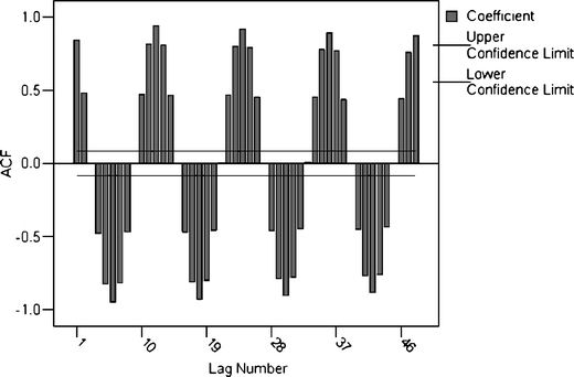

  

  ACF of Sul_M

  Fig. 7

  

  Partial ACF of Sul_M

Analyzing Figs. 4 and 6, small damping of ACF values and the presence of a seasonal component with period 12 in the data series are revealed. So, we consider the series obtained applying a seasonal difference of 12 orders and the mean subtraction. For it, the following model was built:

$$ {X_t} = 0.3626 \times {X_{t - 1}} + {\varepsilon_t} - 1.005 \times {\varepsilon_{t - 1}} $$

where (ε _t ) is the residual with the variance of 2.17.

In Fig. 8, the residual chart is represented. The values of Box–Ljung and MacLeod–Li statistics and the corresponding p values (0.382 and 0.245, respectively), lead us to accept the hypothesis that the residual is a Gaussian white noise. The values of Jarque–Bera statistics confirm these assertions.

Fig. 8

Histogram of residual in the model for Sul_A

Using this model, we forecast the temperatures of the last 120 months using the previous 450 data. The result was good, as it can be seen in Fig. 9.

• The same procedure was followed to detect a good model for Tul_M. After considering a 12-order difference and the mean subtraction, an ARMA(1, 12) model was determined using Akaike selection criterion. It has the equation:

$$ {X_t} = 0.2643 \times {X_{t - 1}} + {\varepsilon_t} - 0.9998 \times {\varepsilon_{t - 1}} $$

where (ε _t ) is a white noise with the variance of 2.878.

Fig. 9

Sul_M: the forecast of temperatures for the last 120 months

The forecast realized taking into account the previous model appears to be close to the registered values (Fig. 10).

Fig. 10

Tul_M: the forecast of temperatures for the last 120 months

4.1.2 GEP models

We performed experiments using the gep package developed for the evolutionary computation software ECJ.¹ In all experiments, we performed 50 independent runs for each setup. The number of genes in a chromosome was set to five in all GEP runs. Each chromosome consisted of five genes, linked in the final model by the addition operator. The head size of a gene was set to five symbols; therefore, the tail size was set to six symbols. In each run, the population consisted of 200 individuals and the algorithm evolved the population over 500 generations. The operator rates used the default values defined in ECJ, which are set as recommended in the literature (Ferreira 2006).

The function set used by the algorithm consisted of {+, −, *, /, sin} where division is implemented as a Koza style protected operator (Koza 1992).

Finding the optimum window size is an optimization problem by itself and there exists no precise algorithm to compute it. Since this is not the main purpose of our article, we do not employ a special algorithm to decide on a specific window size. Instead, we take on a brute-force approach: we perform experiments for all window sizes in the interval $w \in \overline {1,\,6}$. Throughout experiments, we consider the lag k = 1.

The nature of the search process employed by GEP allows it to automatically identify the variables that are most useful to estimate future values among the past n input variables. For example, the window size w = 5 and the lag k = 1 mean that the model may use the most recent five past values x _t − 1,x _t − 2,x _t − 3,x _t − 4,x _t − 5. It is possible that the function identified by GEP as the model that best fits the data does not use some of these variables.

The models obtained are compared with respect to the MSE values obtained on the original data set. In the results, we report the best model (i.e., the model with the smallest MSE value) found in all 50 runs for each window size considered.

For the monthly data, inspired by the best autoregressive models obtained, we also performed experiments for the window size of 12. As expected, the models obtained were more accurate than those obtained for all other window sizes for both Sulina and Tulcea stations. The corresponding charts are presented in Figs. 11 and 12.

Fig. 11

GEP model for Sul_M

Fig. 12

GEP model for Tul_M

In both cases, the residual was Gaussian and homoscedastic. For Sul_A, the residual was correlated with the variance of 3.18, but for Tul_M, it is was independent with the variance of 5.37.

4.2 Models for annual data

4.2.1 ARIMA models

In this section, we present the results obtained for the series of average annual temperatures at Sulina and Tulcea stations, making comparisons with those obtained for the other five stations: Jurilovca—in the Danube Delta, Constanta and Mangalia—on the Black Sea coast, Medgidia and Corugea—in the center of Dobrudja. Since the analysis of mean temperature variation was done in detail in Maftei and Bărbulescu (2008), we restrict ourselves to present the chart of temperature evolution (Figs. 13 and 14).

Fig. 13

Sulina (Sul_A) and Tulcea (Tul_A) annual series

Fig. 14

Medgidia (Med_A), Corugea (Cor_A), Jurilovca (Jur_A), Constanta (Con_A), and Mangalia (Man_A) annual series

It can be seen that there are some series with the same evolution pattern, so we expect to obtain models of the same type. After the application of Kolmogorov–Smirnov test, the normality hypothesis was accepted for all the annual series. The study of the ACF of the series leads us to accept the hypothesis that the data are not correlated. In Figs. 15 and 16, we present, for example, the charts of ACF of Cor_A and Tul_A.

Fig. 15

ACF of Sul_A

Fig. 16

ACF of Tul_A

The results of break tests are listed in Table 1. “Yes” means that the null hypothesis (there is no break in the time series) is accepted, and “no” means that it is rejected, in which case, the break moment is also mentioned.

Table 1 Results of break tests

Since the tests’ results are contradictory, but the majority of them lead us to reject the null hypothesis, the models have been determined for the entire series and for the subseries before and after the break moment.

The best models obtained using the Box–Jenkins methods were:

• 1. Sul_A:

• (a) For Sul_A (1961–2007), after the mean subtraction: a Gaussian white noise with the variance of 0.488.

• (b) For Sul_A (1961–1997), after the mean subtraction:

$$ {X_t} = {\varepsilon_t} - 0.3783 \times {\varepsilon_{t - 3}} $$

where (ε _t ) is a Gaussian white noise with the variance of 0.348 (Fig. 17).

Fig. 17

Sul_A (1961–1997) model

In Table 2, the results of the Kolmogorov–Smirnov test on the residual of the previous MA(3) model are presented.

• (c) For Sul_A (1998–2007):

Table 2 Kolmogorov–Smirnov test for residuals in MA (3) model for Sul_A (1961–1997)

$$ {X_t} = 0.9977 \times {X_{t - 1}} + {\varepsilon_t} $$

where (ε _t ) is a Gaussian white noise with the residual variance of 1.094.

• 2. Tul_A:

• (a) For Tul_A (1961–2007), after the subtraction of the mean: a Gaussian white noise with the variance of 0.516.

• (b) For Tul_A (1961–1997), after the subtraction of the mean: a Gaussian white noise with the variance of 0.422.

• (c) For Tul_A (1998–2007):

$$ {X_t} = 0.9944 \times {X_{t - 1}} + {\varepsilon_t} $$

where (ε _t ) is a Gaussian white noise (Fig. 18).

Fig. 18

Tul_A (1998–2007) model

For the other series located in the Danube Delta and on the Black Sea coast, after some transformation, see Table 3.

• 3. Cor_A:

• (a) For Cor_A (1965–2005), after considering a first-order difference and the mean subtraction:

Table 3 Best models for Jur_A, Con_A, and Man_A

$$ {X_t} = {\varepsilon_t} - 0.8976 \times {\varepsilon_{t - 1}} $$

where (ε _t ) is a white Gaussian noise with the variance of 0.534 (Fig. 19).

• (b) For Cor_A (1965–1997), after considering a first-order difference and the mean subtraction:

Fig. 19

MA(1) model for Cor_A dif 1 (1965–2005)

$$ {X_t} = {\varepsilon_t} - 0.9902 \times {\varepsilon_{t - 1}} $$

where (ε _t ) is a Gaussian white noise with the variance of 0.464 (Fig. 20).

• (c) For Cor_A (1998–2005), after the mean subtraction: a Gaussian white noise with the variance of 0.2073.

• 4. Med_A:

• (a) For Med_A (1965–2005):

Fig. 20

MA(1) model for Cor_A dif 1 (1965–1997)

$$ {Y_t} - 0.833\,{Y_{t - 1}}\, = 9.7725 + {\varepsilon_t},t = \overline {2,\,41} $$

where (ε _t ) is the residual, which is independent, normally distributed.

• (b) For Med_A (1965–1997):

$$ \left( {1 - 0.997B} \right)\left( {1 - B} \right){X_t} = {\varepsilon_t} + 0.909{\varepsilon_{t - 1}}\,,\,t = \overline {2,\,33} $$

where (ε _t ) is a Gaussian white noise.

4.2.2 GEP models

In what follows, the charts presented in Figs. 21, 22, and 23 (corresponding to the Sul_A series) and Figs. 24, 25, and 26 (corresponding to the Tul_A series) provide a good visualization towards how well the GEP models fit the original time series. Excepting the GEP model obtained for Sul_A (1961–1997) for which the residual is dependent, the residuals are Gaussian, independent, and identically distributed. Their variances are, respectively, 0.307, 0.244, and 0.01037 for Sul_A and 0.405, 0.323, and 0.00381 for Tul_A. So, the values are smaller than the corresponding ones in the ARIMA models. The models presented were best among all experiments performed for a given time series (an experiment consists 50 independent GEP runs for each window size).

Fig. 21

GEP_model for Sul_A (1961–2007)

Fig. 22

GEP_model for Sul_A (1961–1997)

Fig. 23

GEP_model for Sul_A (1998–2007)

Fig. 24

GEP_model for Tul_A (1961–2007)

Fig. 25

GEP_model for Tul_A (1961–1997)

Fig. 26

GEP_model for Tul_A (1998–2007)

The solutions obtained by GEP are extremely complex. As reported in the literature, they are useful to fit the time series, but usually shed little light on the nature of the relationship between the variables involved. For example, the model function derived for the series Tul_A (1961–2007) has the expression given below:

$$ \frac{1}{49}\sin \left( {x_{t - 4}^2} \right) * {x_{t - 4}} + \sin \left( {{x_{t - 2}} + {x_{t - 3}}} \right) - \sin \left( {{x_{t - 3}} - {x_{t - 2}}} \right) + $$

$$ + \sin \left( {10 + \frac{{{x_{t - 2}}}}{10}} \right) + \sin \left( {\sin \left( {\sin \left( {\sin \left( {\sin \left( {{x_{t - 4}}} \right)} \right)} \right)} \right)} \right) + {x_{t - 3}}. $$

The MSEs of the GEP solutions presented in the paper are reported in Table 4. For statistical consistency reasons, we also report the mean MSE and the standard deviation (SD) of the MSE over the 50 different runs of the experiment that reported the respective solutions.

Table 4 Mean square errors of GEP models over the time series

It is interesting to note that, in every case, GEP proves to be reliable over the independent runs (the mean is close to the best value, and the SD is small).

We report the iteration number in which the solution was encountered. Also, the last column contains the mean number of iterations needed to obtain the solution over the 50 independent runs of each experiment.

It is interesting to note that the solution is encountered in the second half of the experiment in the majority of cases. This is a proof that the search process is improved over generations in the evolutionary process, and it reaches a good enough solution before the maximum number of generations is reached. Although it exceeds the purpose of our study, it would be interesting to experiment with different GEP settings: for example, to find the appropriate number of generations necessary for the algorithm to run until it reaches convergence. For now, we use GEP settings as recommended in the literature.

5 Conclusions

This study presents the GEP algorithm as a fair competitor of classical methods for the problem of modeling meteorological time series. For the classical models, the residuals were not always homoscedastic or normal, while the errors obtained by GEP models satisfied the conditions of normality, homoscedasticity, and the absence of correlation. Better results were obtained by GEP on time series of smaller size. A straightforward explanation is that data that concerns weather is constantly changing characteristics, which coincides with our intuition that there exist points in meteorological time series when the underlying process changes.

Our results come to support the idea that combining statistical tests for detecting change points with both heuristic methods, such as GEP, and classical Box–Jenkins methods leads to overall better models. The Box–Jenkins models are easier to grasp, while the GEP solutions are much more complex. The advantages of using the GEP metaheuristic are the creativity of the models and, most of all, the lack of constraints imposed on the solution. The functional form of the models obtained with GEP is very complex and hard to understand. Still, for modeling purposes and for the accuracy of the prediction, they prove to be useful.

The analytical expression for the time series shows that nonlinear combinations of the original variables achieve a good level of error reduction. Computation times are bigger than for traditional methods and are not to be neglected when performing time series modeling with GEP, especially for larger data sets.

The evolutionary approach is an attractive alternative to classical methods. The algorithm performs a heuristic search of the best model composed of a set of functions and a set of explanatory variables, guided by an error-based fitness measure. It does not require in advance the specification of the functional form of the model, this way enabling the algorithm to discover alternative nonlinear models that best fit the data set.

In a further study, we shall focus on developing an adaptive method to set parameters for the GEP algorithm. It would be interesting to devise a hybrid method that would combine a heuristic method (e.g., a GA) with statistical procedures to identify the change points. Combined with the constraint-free modeling provided by GEP, the results may be better for long dynamic time series than those obtained by classical approaches.

References

Aksoy H, Gedikli A, Erdem Unal N, Kehagias A (2008) Fast segmentation algorithms for long hydrometeorological time series. Hydrol Process 22(23):4600–4608
Baeck T, Fogel DB, Michalewicz Z (1997) Handbook of evolutionary computation. CRC, Boca Raton
Baltagi BH (2008) Econometrics. Springer, Berlin
Bărbulescu A, Băutu E (2009) ARIMA and GEP models for climate variation. Int J Math Comput (in press)
Bărbulescu A, Ciobanu C (2007) Mathematical characterization of the signals that determine the erosion by cavitation. International Journal Mathematical Manuscripts 1(1):42–48
Brockwell P, Davies R (2002) Introduction to time series. Springer, New York
Buishard TA (1984) Tests for detecting a shift in the mean of hydrological time series. J Hydrol 73:51–69
Charles SP, Bates BC, Smith IN, Hughes JP (2004) Statistical downscaling of observed and modeled atmospheric fields. Hydrol Process 18(8):1373–1394
De Gooijera JG, Hyndman RJ (2006) Twenty five years of time series forecasting. Int J Forecast 22(3):443–473
Ferreira C (2001) Gene expression programming: a new adaptive algorithm for solving problems. Complex Syst 13(2):87–129
Ferreira C (2006) Gene expression programming: mathematical modeling by an artificial intelligence. Springer, Berlin
Gourieroux C, Monfort A (1990) Series temporelles et modeles dynamiques. Economica, Paris
Hubert P, Carbonnel JP (1993) Segmentation des series annuelles de debits de grands fleuves africains. Bull Liaison Com Interafr Étud Hydraul 92:3–10
IPCC (2008) Climate Change and Water, IPCC Technical Paper VI, June 2008, Bates, B.C., Z.W. Kundzewicz, S. Wu and J.P. Palutikof, Eds., IPCC Secretariat, Geneva, 210 pp., Available at http://www.ipcc.ch/ipccreports/technical-papers.htm
Jones PD, Wigley TML, Wright PB (1986) Global temperature variations between 1861 and 1984. Nature 322:430–434
Jones PD (1988) Hemispheric surface air temperature variations: recent trends and an update to 1987. J Climate 1:654–660
Jones PD, Horton EB, Folland CK, Hulme M, Parker DE (1999) The use of indices to identify changes in climatic extremes. Clim Change 42:131–149
Khronostat 1.1 software. Available at http://www.hydrosciences.org
Lee AFS, Heghinian SM (1977) A shift of the mean level in a sequence of independent normal random variables—a Bayesian approach. Technometrics 19(4):503–506
Koza JR (1992) Genetic programming: on the programming of computers by means of natural selection. MIT, Cambridge
Maftei C, Gherghina C, Bărbulescu A (2007) A computer program for statistical analyzes of hydro-meteorological data. International Journal Mathematical Manuscripts 1(1):95–103
Maftei C, Bărbulescu A (2008) Statistical analysis of the climate evolution in Dobrudja region. Lecture Notes in Engineering and Computer Sciences II:1082–1087
Michalewicz Z, Schmidt M, Michalewicz M, Chiriac C (2006) Adaptive business intelligence. Springer, New York
Pettitt AN (1979) A non-parametric approach to the change-point problem. Appl Stat 28(2):126–135
Seskin DJ (2007) Handbook of parametric and nonparametric statistical procedures. CRC, Boca Raton
Taylor W (2000) Change-Point Analyzer 2.0 shareware program. Taylor Enterprises, Libertyville. Available at http://www.variation.com/cpa
Wagner N, Michalewicz Z, Khouja M, Mcgregor RR (2007) Time series forecasting for dynamic environments: the DyFor genetic program model. IEEE Trans Evol Comput 11(4):433–452
Acknowledgements
This paper was supported by grant ID_262 and grant PNCDI2 NatCOMP 11028/2007.
Author information
Authors and Affiliations
Corresponding author
Rights and permissions
About this article
Cite this article
Bărbulescu, A., Băutu, E. Mathematical models of climate evolution in Dobrudja. Theor Appl Climatol 100, 29–44 (2010). https://doi.org/10.1007/s00704-009-0160-7
Received:
Accepted:
Published:
Issue Date:
DOI: https://doi.org/10.1007/s00704-009-0160-7