
Abstract
We propose a novel parallel image space adaptive rendering approach. Contourlet transform which includes Laplacian pyramid and directional filter banks is modified for multi-scale and directional analysis in our algorithm. In sampling stage, the image space is coarsely sampled first. The sampled image is analyzed into coarse and difference values in multi-scale using Laplacian pyramid transform. Based on the analysis, a heuristic method is proposed to repeatedly distribute adaptive Monte Carlo samples. In reconstruction stage, the final image is reconstructed by filtering each pixel using our anisotropic per-pixel filter. The filter size depends on the variance and attenuation values. The filter’s anisotropic property is computed by the directional filter banks. Compared to the state-of-the-art image space adaptive rendering methods, the results rendered by our algorithm show improvement in both visual image quality and numerical error while using sparse samples.
1 Introduction
Physically based photo-realistic images are rendered by integrating all the light transmission, absorption, emission, reflection and refraction between the objects of different materials and textures in the scene through camera screen. Because the dimension of this integration is almost infinite, an ideal image is difficult to be generated. Monte Carlo methods can be used to render an approximate result. The quality of the image depends on the number of samples in each pixel and it is expensive to render using many samples. In order to generate a high-quality image with sparse samples, different adaptive sampling and reconstruction methods are employed.
There are two kinds of adaptive sampling methods: multidimensional sampling and image space sampling. Compared with multidimensional adaptive methods which always suffer the curse of dimensionality, the image space methods are more efficient and widely used. Their inputs are only the contribution of the samples and their outputs are the position of the adaptive samples. The process of the ray tracing is traded like a black box, so it can be widely used in Monte Carlo rendering engines with different ray tracing techniques.
The image space adaptive sampling methods locate Monte Carlo samples in an optimal fashion way and always apply a suitable filter to decrease the variance in the integrand. Most of these methods use local variance value [1] to build their heuristic strategies. This kind of strategies only focus on the local variation and ignore the smooth varying. Wavelet analysis is introduced to solve this problem [2], but it causes an evident aliasing of sampling distribution. To reconstruct an ideal result, different kinds of reconstruction methods are used. The wavelet reconstruction removes the high frequency signal to smooth the image, but it may cause block effect. The square filters reconstruct smooth results with no block effect [3], but most square filters are isotropic which may cause aliasing on the discontinuities of the image.
Motivated by this observation, we propose a parallel image space adaptive rendering approach based on the multi-scale and directional analysis. Contourlet transform is introduced into our algorithm: Laplacian pyramid helps to adaptively sample the image and directional filter banks are used to build filters. In summary, our algorithm has the following contributions:
- Heuristic sampling method :
-
Based on the Laplacian pyramid transform, we analyze the sampled image plane in multi-scale and propose a novel sampling method. Our heuristic method generates good quality sampling distribution which focuses on both the local variance and the variance in non-image dimensions. A new strategy is also introduced to avoid the sampling distribution aliasing which happens in multi-scale analysis sampling such as adaptive wavelet rendering method [2].
- Anisotropic per-pixel filter :
-
Depending on the complexity and directionality features in the image, our anisotropic per-pixel filters are built by analyzed information of the sampled image such as variance and the directional filter banks.
2 Previous work
Our algorithm has been inspired by previous work on image processing, multi-scale analysis, adaptive sampling as well as filter techniques.
Adaptive sampling technique shows more advantages than traditional stochastic sampling. It varies the sampling rate due to the frequency of rendering space. There are two categories of adaptive sampling method: image space sampling and multidimensional space sampling. To render the effects such as motion blur, depth of field and soft shadows, multidimensional methods locate adaptive samples in the multidimensional space. Soler et al. [4] give an approach to render high-quality depth of field effect based on sampling image and lens dimensions. By using Fourier transform to analyze the image and time dimensions, Egan et al. [5] adaptively sample and reconstruct motion blur effect. But their methods can only focus on one effect. Hachisuka et al. [6] present a general multidimensional sampling method to generate high-quality results, but it costs a lot of time and memory to calculate and save the multidimensional information when the dimension increases.
Because of the curse of dimensionality and the one effect limitation of some multidimensional sampling methods, the image space adaptive sampling strategies [7, 8] are more widely used and effective. Mitchell [1, 9] first proposed an adaptive technique based on the mean square error. Rousselle et al. [3, 10] adaptively generated samples to minimize the local mean square errors.
As an independent part of rendering, reconstruction has been studied by many researchers. Most multidimensional algorithms have their own reconstruction methods. Shirley et al. [11] adaptively filtered the image using a depth buffer. Egan et al. [12] proposed a method to render soft shadows depending on image and area light surface space analysis. But they focus on only one effect. The reconstruction method proposed by Lehtinen et al. [13, 14] generates better results, but this method needs additional information such as speed and depth of the samples. Li et al. [15] also generate an anisotropic filter, but it is based on the information such as normal, texture and depth. Our method trades the ray tracing technique as a back box and can be widely used in many rendering engines.
Image processing methods are also effective in image space reconstruction. Dammertz et al. present a fast and simple ‘a Trous” filtering method for global illumination images [16]. Portilla et al. [17] use an approach which denoises the image in wavelet domain. Wavelet synthesis introduced by Overbeck et al. [2] is used to remove the high frequency signal which is considered as noises.
3 Overview
There are two main stages in our algorithm: sampling and reconstruction. The framework is shown in Fig. 1. At the beginning of our rendering process, the entire image space is divided into equal-sized square tiles. In sampling stage, first this board is coarsely sampled to get the contributions of every pieces in it. Second, the sampled image board is analyzed into multi-scale coarse and difference values by Laplacian pyramid (LP) in iteration. The coarse values are considered as the input image of each iteration and the difference values are considered as the prediction error. In order to build our heuristic priority value of each pixel, the variance and attenuation information is calculated from the coarse values. Third, the area of each scale having the maximum priority value is sampled and this area is updated after sampling. This sampling step is repeated until a termination criterion is fulfilled.

The framework of our algorithm
In reconstruction stage, we generate anisotropic filters for every pixels of the image. The size of each filter is decided by the variance and attenuation values of the sampled image. The directional information is calculated by analyzing the difference values using directional filter banks (DFBs). The final result is synthesized by filtering each pixel using its suitable anisotropic per-pixel filter.
3.1 The multi-scale and directional analysis process
To effectively sample the complexity and directionality features in the image space, contourlet transform [18] is introduced into our algorithm. Because of our rendering framework, contourlet transform is modified and separated into two parts: LP analysis and DFB process. LP is used to adaptively sample the image and DFBs are used to build the anisotropic per-pixel filter (in Fig. 2). We propose two key extensions to the original contourlet transform that allow us to use it effectively in our adaptive rendering framework: implement the LP transform in iteration and resize the output signal.

The orange lines represent the multi-scale analysis process in sampling stage and the blue lines represent the directional analysis process in reconstruction stage
LP is a powerful tool in digital signal processing. In this article, it is used to iteratively capture the multi-scale coarse and difference values of the image. At the beginning of each iteration, four images \(f^{i,j}_{k}\) are generated from the input sampled image f k . After filtered by an analysis filter H and downsampled, these four images are combined into one. This combined image is the coarse value of scale k and the input of the next iteration k+1. The difference values d k are generated by subtracting the input image f k with the values which are obtained by upsampling \(\tilde{f}^{0,0}_{k}\) and filtering it by a synthesis filter G. The size of the output signals is the same as the input image which is different from the original contourlet transform.
Directionality is a crucial factor in image reconstruction. DFBs are used to calculate directional information of the difference values which are computed in sampling stage. The difference values d k are decomposed into 2l−1 directionality subbands by filter S n . The decomposition level l k is user defined, typically it is 1−3. The filter S i represents the DFB process. The result D i is the directionality subbands of the image pixel and is used to build our anisotropic per-pixel filter.
4 Adaptive sampling
4.1 Initialization
We assume the whole image plane as a tessellation board. It is combined by equal-size square pieces each of which is considered as the smallest unit during our analysis process. The size of each piece is proportional to the pixel, such as one pixel or a quarter pixel. Each piece contains the mean contribution, maximum and minimum sample contribution of its image area. Our algorithm begins with a initial sampling. Each piece of the board is sampled at least one sample in its area and the jittering sampling strategy is used to avoid aliasing. After initial sampling, this board as a two-dimensional discrete image will be analyzed by LP in the following step. The entire analysis stage is shown in Fig. 3.

(a) The tessellation board (gray line) on a image (red line), the piece size is a quarter pixel. We filter the pieces from level 1 to level k, the size of filter in level k being 2k. (b) The input image is analyzed into several information of each level such as coarse values, difference values, attenuation values and variance values. They are used to generate the priority values from level 1 to level k by our heuristic method. (c) The same region may have different priority values in different levels
4.2 Multi-scale analysis
To adaptively sample in both rapid changing and smooth regions of high-dimensional variance, we analyze the coarsely sampled image into multi-scale values. LP is used to decompose the input image into coarse values and difference values from level 1 to level k.
Overbeck et al. [2] proposed a wavelet analysis method for adaptive rendering, but its sample distribution has aliasing since they do not analyze the contribution value of all positions in large scales. To avoid this kind of aliasing, we first generate four images \(f^{i,j}_{k}\) from the input sampled image by moving the board position.
Here, f k (x,y) represents the input image board of level k in the analysis iteration; f 0 is the initial coarsely sampled image board. Second, each generated image is processed by low-pass filter H and downsampled.
The size of the output \(\tilde{f}^{i,j}_{k}(x,y)\) is one quarter of the original input image and these output images are combined into a new image.
Here, f k+1(x,y) is the coarse value of level k and it is the input image of the next level k+1 in our analysis process. Each piece of the current coarse image contains the coarse contribution of the area whose center is (x,y) and the size is 2k. Because of the image generation and combination, the input image size of the level k+1 is the same as the image size of level k and the input image of each scale has the value of all positions which allows to avoid the sampling aliasing which took place in the previous adaptive wavelet rendering method.
To get the difference value, the output signal \(\tilde {f}^{0,0}_{k}(x,y)\) is upsampled and filtered by a high-pass filter G. The difference value d k (x,y) is obtained by subtracting this filtered result with the original input image f k (x,y).

The requirement for LP process is the orthogonality condition on the filters H and G. In this article, we also need ∑h(z)=1. To implement H and G, there are many filters [19] which can be used, such as Haar, 5-3, 9-7 or DB3.
4.3 Heuristic priority
After the multi-scale analysis, a priority queue is built for adaptive sampling. The priority queue is combined by the priority value of every pieces on the board from level 1 to level k. In the repeatedly sampling step, we sample the region having the maximum priority value. Monte Carlo samples located in this region are based on some special distributions such as random or Poison disk distribution. When a region has been sampled, we re-analyze this region from level 1 to level k and update its priority value. The image board is repeatedly sampled until a termination criterion is fulfilled, such that the given sample budget has been all used. The priority value is calculated by a heuristic method shown in (5).
The heuristic property value P k (x,y) of coordinate (x,y) in board plane of level k is defined by three factors of this region: the variance, the difference value and the attenuation value. The variance and difference factors give the region which is need to be sampled: V k (x,y) shows the complexity of the region and d k (x,y) shows the rapidly changing region. The attenuation value A k (x,y) shows the sampling efficiency of the region and it is used as the weight of the other two elements.
The variance value V k (x,y) is the square of the contrast metric used by Mitchell [1]. V k (x,y) represents the complexity feature in the region in coordinate (x,y) of level k.
Here, R k,x,y is the level k region of coordinate (x,y); V k (x,y) is calculated by summing all the variances of every pieces in region R k,x,y ; N is the number of the pieces in R k,x,y ; I max and I min are the maximum and minimum sample contribution saved in each piece.
In general, every pixel of the ideal result will converge to a stable color. During the sampling stage, we compute the converging speed of each region and put samples on the regions whose converging speeds are high. The attenuation value shows which region is changing rapidly. To compute the converging speed, we heuristically accumulate the differences between the current and last coarse value of each multi-scale region.


The attenuation value in coordinate (x,y) of level k is computed by F k (x,y) and α, which controls the sensitivity of the attenuation value; typically it is 0.3–0.5. \(A^{\prime}_{k}(x,y)\) is its last attenuation value in coordinate (x,y) of level k. F k (x,y) is the difference between the current coarse value f k (x,y) and its last value \(f^{\prime}_{k}(x,y)\) in coordinate (x,y) of level k. In implementation, when the max iteration level k is 3–5, our algorithm gives high-quality results. In our experiments, we define the iteration level to be 4.
5 Reconstruction
To reconstruct the ideal image, we want to filter the noises and preserve the details using our method. The samples in the image space always have the same or similar contribution with their neighbors, such as in the same material or the same texture of the objects, in the motion blur region, depth of field area or soft shadows. It means this kind of pixels can share samples with their neighbors. So, a novel anisotropic per-pixel filter is presented by our algorithm. Each pixel of the final image has its own filter. The results analyzed during sampling stage are used to calculate the size and directional information of our anisotropic per-pixel filter (in Fig. 4).

(a) The difference values are the input of the DFB process. (b) The frequency partitioning of directional filter banks where l=2,3 and there are 4 and 8 real wedge-shaped frequency bands. (c) The directionality subbands of the input difference values after filtering by the DFBs. (d) The filter size is calculated by the information which is calculated during sampling stage. (e) Using the directional and size information, the final image is reconstructed by our anisotropic per-pixel filters
5.1 Filter size
A suitable size of our anisotropic per-pixel filter is calculated first. If the pixel is in smooth area like motion blur or soft shadows, its filter size will be large because these pixels share a lot of samples with its neighbors. If the pixel is in a sharp area like an edge, its filter size will be small because this kind of pixels share a few or no samples with its neighbors. The size of each filters is decided by the variance, attenuation and coarse values of its pixel. Rousselle et al. propose a method to calculate a square filter using the variance value [3]. It greedily minimizes the mean square error of the image. Sen and Darabi introduced information theory to filter the noises [20]. Their method considers the relationship between the random property of the input samples and their output contributions. Inspired by their approaches, we include not only the variance values, but also the attenuation values. The variance represents the complexity of the filter regions and the attenuation value shows the bias of their colors. For each pixel, a threshold value is computed by our algorithm through level 1 to k. This threshold is calculated from level 0 to k. If the current threshold T k (x,y) is positive, the scale size 2k of level k is decided to be the filter size. The threshold is calculated by the following equation.
T k (x,y) is the threshold in pixel (x,y) of level k. V k is the variance value, A k is the attenuation value and f k is the coarse value in pixel (x,y) of level k. We use A k instead of the scale size which was used in Rousselle et al.’s method [3], because it can identify the size of rapid changing area and show good results.
5.2 Directional information
In the region of a pixel filter, this pixel always shares samples with its neighbors in some certain directions. For example, the motion blur region has its moving direction and the border of the object has its shape direction. DFBs are used to get these directional information [18, 21]. DFBs are efficiently implemented via a l-level tree structured decomposition that leads to 2l subbands with wedge shaped frequency partition as shown in Fig. 4. DFBs are employed in our algorithm to analyze the difference values into 4–8 directionality subbands.
In order to obtain four directionality subbands from the input values, the first two decomposition levels of the DFB process are given in Fig. 5. The fan filters and the quincunx filter banks (QFBs) Q 0,Q 1 are used as this process shows. The outputs from 0 to 3 are the four directionality subbands.

The first two levels of DFB process. At each level, QFBs and fan filters are used to filter the input image. The deep purple regions represent the ideal frequency supports of the filter
To obtain 8 or more directions information of the input values, a third level of the DFB process is added. Figure 6 shows the first two channels of the third level. They are linked after the second level of the first two channels in Fig. 5. The other two channels of third level are the same as the first two except for exchanging the filters R 0,R 1 with R 2,R 3. The outputs are the 8 directionality subbands.

The analysis of the two resampled QFBs that are used from the third level in the first two channels of the DFB process
The matrices used in the DFB process are shown below. Q 0 and Q 1 are the QFBs; R 0,R 1,R 2 and R 3 are used to provide the equivalence of the rotation operations.

This DFB process has one input and 2l−1 outputs as shown in the multi-scale and directional analysis process (Fig. 2). The input is the difference values d k . Each channel of the DFB process is considered as an \(S_{2^{l}-1}\) filter and the directionality subband is \(D_{2^{l}-1}\).
5.3 Anisotropic per-pixel filter
After computing the size and directionality subbands, the anisotropic per-pixel filters centered on each pixel are generated. In the filter region, we compute a weight of each sample. The weight is different in different directions of the filter according to the anisotropic property.
We loop over all the samples in the filter region R x,y to compute their weights ω s and use these weights to blend the color of pixel (x,y). The size of filter region R x,y is calculated by (9). The weight of each sample is determined by its distance from the pixel center and its directionality subbands.
Gaussian function is used to ensure the smoothness of the filter; \(\operatorname {dis}(s)\) is the distance between sample s and the current integrating pixel; δ s is the anisotropic value of this sample.
Sample s is being located between two directions, i and i+1 in R x,y ; dir i is the value of directionality subband i; β i is the angle of the direction i; β s is the direction angle of s in R x,y and its value is between β i and β i+1; and δ s is the interpolation of the two directional values.
5.4 Parallelization
Since the adaptive rendering methods need feedback of the previous information of the whole space in each sampling iteration, there are few adaptive sampling methods. Depending on our tessellation construction, parallelization can be easily introduced to our algorithm. We separate the tessellation board into equal-size parts to independently render them in parallel. Because each part is independently sampled and reconstructed as described above, the size of these parts cannot be smaller than the maximum scale of the multi-scale LP analysis. To ensure the adaptive sampling property, a strategy is used to assign each part a sample budget after the initialization step. If the part has complexity features, the sample budget is large. Otherwise, the sample budget is small. Liu et al. proposed a strategy to adaptively sample multidimensional space in parallel [22] by using kd-tree structure. Inspired by their strategy, we propose a method to assign each square part a sample budget.
Here, B Ω is the sample budget assigned to the parallel part Ω, N T is the total sample count, P k (x,y) is the priority value (in (5)) which is the priority value of the scale region in coordinate (x,y) of level k after initialization step, and P total=∑P k is the total priority value. After initialization of our algorithm, we separate the tessellation board and assign each part a sample budget. Each part is rendered independently using our approach until the assigned samples have all been used. Because of our parallelization strategy, the whole sample distribution is adaptive.
6 Implementation and results
Our algorithm and previous approaches are implemented on LuxRender [23]. All results were rendered on a Intel Core i7 CPU at 2.80 GHz with 2 GB of RAM. In this section, the effects of multi-scale sampling, anisotropic per-pixel filters and parallel strategy in our algorithm are analyzed. The sample distribution and image quality are separately compared between our approach and previous image space adaptive sampling methods such as the Mitchell method [1], adaptive wavelet rendering (AWR) [2] and the state-of-the-art method of greedy error minimization (GEM) [3].
6.1 Algorithm analysis
- Filters in multi-scale analysis :
-
The filters H and G used in LP process affect the multi-scale analysis. Different filters give different priority values. During the sampling stage, using different filters such as Haar, 5-3, 9-7 or DB3 causes different sample distributions.
Figure 7 shows the different sample distributions of the kitchen table scene. The resolution of these images is 400×400. Each image uses four samples per pixel. Table 1 gives the sample count of different filters in all levels. The data illustrate that DB3 filter gives a rough sample distribution and put more samples in the large-scale regions. Haar filter gives a smoother sample distribution than DB3. The 9-7 filter focuses on the discontinuities of the image and so does the 5-3 filter, but the 5-3 filter puts more samples in the large-scale regions. Figure 8(a) shows that the result of filter 5-3 has the least mean square error (MSE). But with the sample per pixel increasing, these differences are trifling. In the following experiments, we use 5-3 filter in multi-scale analysis process.
Fig. 7 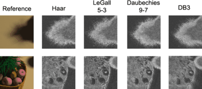
The reference image and the sampling distributions of the kitchen table scene generated by using different filters
Fig. 8 
(a) The MSE values by using different filters in our multi-scale analysis process. (b) Comparison of the sampled image quality without reconstruction step of our method and previous adaptive methods. (c) The effect of our anisotropic per-pixel filter by rendering the ball scene
Table 1 The sample counts of different filters in different level - Sample distribution :
-
To use the image space sampling methods, sample distribution is very important for rendering a high-quality image, because in most rendering methods the sampling stage is separated from the reconstruction stage and it can do anti-aliasing and remove the noises. Figure 9 illustrates the sample distributions of Mitchell method, AWR, GEM and our algorithm by rendering the chess scene in a 512×512 resolution with 16 samples per pixel.
Fig. 9 
The sampling distributions of Mitchell, AWR, GEM and our method
The results show that our distribution focuses on both rapid changing areas and soft shadows of the image while using the same samples as in other methods. Mitchell method samples the image based on the pixel variance which causes it to ignore variance in the large scale. The distribution of GEM shows that it puts too many samples on the soft shadows to pursue a local optimization and ignores the edge of the chess. The AWR distribution has aliasing in the large-scale regions. The MSE values in Fig. 8(b) show that our approach gives a better result. These MSE values are calculated from the images rendered without their reconstruction steps.
- Anisotropic filter :
-
The effect of our anisotropic per-pixel filter is shown in Fig. 10 by rendering the billiard ball scene and the kitchen table scene. Each image is rendered at 512×512 resolution with four samples per pixel. The results with using filter are much better than the results without one. The MSE values of the ball scene are shown in Fig. 8c. Our anisotropic per-pixel filter works reasonably well for both the motion blurred regions and soft shadow regions.
Fig. 10 
(Left) The images are rendered by our algorithm with no reconstruction step. (Middle) The images are rendered by our algorithm with the anisotropic per-pixel filter. (Right) The reference images
- Parallel implementation :
-
We analyze the parallel strategy of our algorithm. The experiments of the given kitchen scene are rendered at 512×512 resolution using the original strategy and the parallel strategy (in Fig. 11). The speed, MSE and sampling distributions are compared. Figure 11(a) shows that our algorithm runs faster with threads increasing. The sampling distributions show the effect of separating the image space into different size parts. If we separate the image plane into small parts, the sample distribution has strong aliasing on the part borders. But the MSE values show that the separating strategy does not considerably affect the image quality (in Fig. 11(b)). Using eight threads, our algorithm runs 2–4 times faster than using one thread, depending on different scenes.
Fig. 11 
(a) The cost time of rendering the same scene using different threads. (b) The MSE value of these results. (c) The sample distribution which is generated by separating the image into parallel parts of 64×64 pixels, while (d) is generated by separating the image into parallel parts of 16×16 pixels. (e) The distribution of our algorithm without the parallel strategy. (f) The reference image


6.2 Results
The results of image quality comparison of our algorithm and previous methods such as Mitchell adaptive sampling, AWR method and GEM method are shown in Fig. 12. The time shown in the figure refers to the whole rendering process.

All images are rendered at 1024×1024. Top row is a 4D scene with depth of field. The bottom row is a 6D scene with depth of field and area lighting. The images rendered by our algorithm are better than these of previous image space adaptive methods and cost much less time by using our parallel strategy
Figure 12(a) is a chess scene with depth of field effect. This scene is combined with white and black chessmen. The focus of the camera is on the black bishop in the center. The resolution of the rendered images is 1024×1024. Each image uses eight samples per pixel. On the region of depth of field, GEM method filters a better result than Mitchell method. AWR method reconstructs a smooth blur effect. Compared with these previous methods, our method achieves a near-reference quality image.
Figure 12(b) is a billiards pool scene with depth of field and soft shadows effect. There are two area lights in this scene and the focus is on the purple ball in the center. The resolution of the rendered images is 1024×1024. Each method uses eight samples per pixel. The result rendered by Mitchell method has rough shadows and a lot of high light noises. AWR method reconstructs a better result of soft shadows, but it has block effect with high light noises. GEM method filters the noises based on minimizing the MSE value, but it cannot reconstruct high-quality discontinuities of the image. Our method renders a better result than these previous methods in both the blur regions and the soft shadows. The results of these two scenes show that the images rendered by our parallel strategy cost much less time and still have a better effect.
7 Conclusion and future work
In this paper, a novel adaptive rendering algorithm is presented to sample and reconstruct high-quality images using multi-scale and directional analysis. Laplacian pyramid is employed to analyze the image in multi-scale and a heuristic method is used to adaptively sample the image space. In reconstruction stage, we generate anisotropic per-pixel filters to filter the image based on previous analysis and directional filter banks. A parallel strategy is introduced to implement our approach in parallel. The results rendered by our algorithm have better quality images than that of the previous image space adaptive methods.
A drawback of LP is implicit over-sampling and it is usually used in image processing. We consider to improve the multi-scale analysis process by analyzing data in other dimensions such as time or lens with no over-sampling. The output of DFB process has fixed directions such as 4 or 8. We plan to build a finer anisotropic filter with no direction and dimension limitations.
References
Mitchell, D.P.: Generating antialiased images at low sampling densities. In: Proceedings of the ACM SIGGRAPH’87, Anaheim. Annual Conference Series, vol. 21, pp. 65–72. ACM, New York (1987)
Overbeck, R.S., Donner, C., Ramamoorthi, R.: Adaptive wavelet rendering. ACM Trans. Graph. 28(5), 1–12 (2009). Proceedings of the ACM SIGGRAPH Asia Conference
Rousselle, F., Knaus, C., Zwicker, M.: Adaptive sampling and recounstruction using greedy error minimization. ACM Trans. Graph. 5(3), 1–10 (2011). Proceedings of the SIGGRAPH Asia Conference
Soler, C., Subr, K., Durand, F., Holzschuch, N., Sillion, F.: Fourier depth of field. ACM Trans. Graph. 28(2), 1–12 (2009). Proceedings of the SIGGRAPH Conference
Egan, K., Tseng, Y.T., Holzschuch, N., Durand, F., Ramamoorthi, R.: Frequency analysis and sheared reconstruction for rendering motion blur. ACM Trans. Graph. 28(3), 1–13 (2009). Proceedings of the SIGGRAPH Conference
Hachisuka, T., Jarosz, W., Weistroffer, R.P., Dale, K.: Multidimensional adaptive sampling and reconstruction for ray tracing. ACM Trans. Graph. 27(3), 33 (2008). Proceedings of the SIGGRAPH Conference
Jin, B., Ihm, I., Chang, B., Park, C., Lee, W., Jung, S.: Selective and adaptive supersampling for realtime ray tracing. In: Proceedings of the Conference on High Performance Graphics, pp. 117–125 (2009)
Genetti, J.D., Gordon, D., Williams, G.: Adaptive supersampling in object space using pyramidal rays. Comput. Graph. Forum 17(1), 29–54 (1998)
Mitchell, D.P.: Spectrally optimal sampling for distribution ray tracing. In: Computer Graphics Proceedings, ACM SIGGRAPH, Las Vegas. Annual Conference Series, vol. 25, pp. 157–164. ACM, New York (1991)
Rousselle, F., Knaus, C., Zwicker, M.: Adaptive rendering with non-local means filtering. ACM Trans. Graph. (2012). Proceedings of the SIGGRAPH Asia Conference
Shirley, P., Alila, T., Cohen, J., Enderton, E., Laine, S., Luebke, D., McGuire, M.: A local image reconstruction algorithm for stochastic rendering. In: Symposium on Interactive 3D Graphics and Games (I3D’11), pp. 9–14. ACM, New York (2011)
Egan, K., Hecht, F., Durand, F., Ramamoorthi, R.: Frequency analysis and sheared filtering for shadow light fields of complex occluders. ACM Trans. Graph. 30(4) (2011)
Lehtinen, J., Alia, T., Chen, J., Laine, S., Durand, F.: Temporal light field reconstruction for rendering distribution effects. ACM Trans. Graph. 30(4) (2011)
Lehtinen, J., Alia, T., Laine, S., Durand, F.: Reconstructing the indirect light field for global illumination. ACM Trans. Graph. (2012)
Li, T.M., Wu, Y.T., Chuang, Y.Y.: Sure-based optimization for adaptive sampling and reconstruction ACM Trans. Graph. 31(6), 186 (2012). Proceedings of ACM SIGGRAPH Asia 2012
Dammertz, H., Sewtz, D., Hanika, J., Lensch, H.P.A.: Edge-avoiding a-trous wavelet transform for fast global illumination filtering. In: Proceedings of the Conference on High Performance Graphics, Eurographics Association (HPG’10), Aire-la-Ville, Switzerland, pp. 67–75 (2010)
Portilla, J., Strela, V., Wainwright, M.J., Simoncelli, E.P.: Image denoising using scale mixtures of gaussians in the wavelet domain. IEEE Trans. Image Process. 12(11), 1338–1351 (2003)
Do, M.N., Vetterli, M.: The contourlet transform: an efficient directional multiresolution image representation. IEEE Trans. Image Process. 14(12), 2091–2106 (2005)
Skodras, A., Christopoulos, C., Ebrahimi, T.: The jpeg 2000 still image compression standard. IEEE Signal Process. Mag. 18(5), 36–58 (2001)
Sen, P., Darabi, S.: On filtering the noise from the random parameters in monte carlo rendering. ACM Trans. Graph. (2012). Proceedings of the SIGGRAPH Conference
Park, S.I., Simith, M.J.T., Mersereau, R.M.: Improved structure of maximally decimated directional filter banks for spatial image analysis. IEEE Trans. Image Process. 13, 1424–1431 (2004)
Liu, X.D., Wu, J.Z., Zheng, C.W.: Kd-tree based parallel adaptive rendering. Vis. Comput. 28(6–8), 613–623 (2012)
http://src.luxrender.net (2008)
Author information
Authors and Affiliations
Corresponding author
Rights and permissions
About this article
Cite this article
Liu, X.D., Zheng, C.W. Parallel adaptive sampling and reconstruction using multi-scale and directional analysis. Vis Comput 29, 501–511 (2013). https://doi.org/10.1007/s00371-013-0814-4
Published:
Issue Date:
DOI: https://doi.org/10.1007/s00371-013-0814-4