Saliency for image manipulation

Abstract

Every picture tells a story. In photography, the story is portrayed by a composition of objects, commonly referred to as the subjects of the piece. Were we to remove these objects, the story would be lost. When manipulating images, either for artistic rendering or cropping, it is crucial that the story of the piece remains intact. As a result, the knowledge of the location of these prominent objects is essential. We propose an approach for saliency detection that combines previously suggested patch distinctness with an object probability map. The object probability map infers the most probable locations of the subjects of the photograph according to highly distinct salient cues. The benefits of the proposed approach are demonstrated through state-of-the-art results on common data sets. We further show the benefit of our method in various manipulations of real-world photographs while preserving their meaning.

1 Introduction

Is a picture, indeed, worth a thousand words? According to a survey of 18 participants, when asked to provide a descriptive title for an assortment of 62 images taken from [13], on average, an image was described in up to four nouns. For example, 94.44 % of the participants referred to the foreground ship to describe the top-left image in Fig. 1, 50 % referred to the background ship as well, 55.55 % mentioned the harbor and a mere 27.7 % pointed out the sea. In [15], prediction of human fixation points was highly improved when recognition of objects such as cars, faces and pedestrians was integrated into their framework. This further shows that viewers’ attention is drawn towards prominent objects which convey the story of the photograph. It is clear from these results that when manipulating images, in order to preserve the meaning of the photograph, it is crucial that these singled-out objects remain intact.

Fig. 1

Story preserving artistic rendering (Top) “Ships near a harbor.” (Top-right) Painterly rendering. Details of prominent objects are preserved (ships and harbor), while non-salient detail is abstracted away using a coarser brush stroke. (Bottom) “Girl with a birthday cake.” (Bottom-right) A ic using flower images. Non-salient detail is abstracted away using larger building-blocks, whereas salient detail is preserved using fine building-blocks

Our goal is the detection of pixels which are crucial in the composition of a photograph. One way to do this would be to apply numerous object recognizers, an extremely time-consuming task, usually rendering the application unrealistic. In this paper, we suggest the use of a saliency detection algorithm to detect the said crucial pixels.

Currently, the three most common saliency detection approaches are: (i) human fixation detection [5, 11, 14, 19], (ii) single dominant region detection [10, 13, 16], and (iii) context-aware saliency detection [9]. Human fixation detection results in crude inaccurate maps which are inadequate for our needs. A single dominant region detection is insufficient when dealing with real-world photographs which may consist of more than a single dominant region. Our work is mostly inspired by [9], but unlike them we detect the salient pixels which construct the prominent objects precisely, discarding their surroundings (see Fig. 2).

Fig. 2

Precise detection. Our algorithm detects mostly the objects, whereas [9] detects also parts of the background

We propose an approach for saliency detection in which we construct for each image a prominent-object arrangement map, predicting the locations in the image where prominent objects are most likely to appear.

We introduce two novel principles, object association and multi-layer saliency. The object association principle incorporates the understanding that pixels are not independent and most commonly, adjacent pixels will pertain to the same object. Utilizing this principle, we are able to successfully predict the location of prominent objects portrayed in the photograph. In addition, we understand that the duration in which an observer views an image will affect the areas he regards as salient. We therefore, introduce a novel saliency map representation which consists of multiple layers, each layer corresponding to a different saliency relaxation. We especially benefit from this multi-layer saliency principle when creating different layers of abstractions in our painterly rendering application.

In addition to these two principles, we incorporate two principles suggested in [9]—pixel distinctness and pixel reciprocity—for which we propose a different realization. We argue that our realization offers a higher precision in a shorter running time.

Our method yields three representations of saliency maps: a fine detailed map which emphasizes only the most crucial pixels such as object boundaries and salient detail; a coarse map which emphasizes the prominent objects’ enclosed pixels as well; and a multi-layered map which realizes the multi-layer saliency principle. We demonstrate the benefits of each of the representations via three example applications: painterly rendering, image mosaicing, and cropping.

Our contributions are threefold. First, we define four principles of saliency (Sect. 2). Second, based on these principles, we present an algorithm for computing the various saliency map representations (Sects. 3, 4). We show empirically that our approach yields state-of-the-art results on conventional data sets (Sect. 5). Third, we demonstrate a few possible applications of image manipulation (Sect. 6).

2 Principles

Our saliency detection approach is based on four principles: pixel distinctness, pixel reciprocity, object association and multi-layer saliency.

• (1) Pixel distinctness relates to the tendency of a viewer to be drawn to differences. This principle was previously adopted for saliency estimation by [4, 9, 13]. We propose a different realization obtaining higher accuracy in a shorter running time.

• (2) Pixel reciprocity argues that pixels are not independent of each other. Pixels in proximity to highly distinctive pixels are likely to be more salient than pixels that are farther away [9]. Since distinctive pixels tend to lie on prominent objects, this principle further emphasizes pixels in their vicinity.

• (3) Object association suggests that viewers tend to group items located in close proximity, into objects [17, 20]. As illustrated in Fig. 3, the sets of disconnected dots are perceived as two objects. The object association principle captures this phenomenon.

  Fig. 3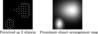

  

  Object association: Viewers perceive the left image as two objects. Our result (right) captures this

• (4) Multi-layer saliency maps contain layers which correspond to different levels of saliency relaxation. The top layers emphasize mostly the dominant objects, while the lower levels capture more objects and their context, as illustrated in Fig. 4.

  Fig. 4

  

  Our multi-layer saliency. Each layer reveals more objects, starting from just the leaf, then adding its branch and finally adding the other branch

3 Basic saliency map

The basis for all of our saliency representations is the Basic saliency map. Its construction consists of two steps (Fig. 5): construction of a distinctness map, D, based on the first and second principles, followed by an estimation of a prominent object probability map, O, based on the third principle. The two maps are merged together into the Basic saliency map:

(1)

where S _b (i) is the saliency value for pixel i. Being a relative metric, we normalize its values to the range of [0,1].

Fig. 5

Basic saliency map construction. The Basic saliency map, S _b in (d), is the product of the Distinctness map, D in (b), and the Object probability map, O in (c). While the Distinctness map (b) emphasizes many pixels on the grass as salient, these pixels are attenuated in the resulting map, S _b  (d), since the grass is excluded from O (c)

3.1 Distinctness map

We construct the Distinctness map in two steps: computation of pixel distinctness, followed by application of the pixel reciprocity principle.

Estimating pixel distinctness: The pixel distinctness estimation is inspired by [9], where a pixel is considered distinct if its surrounding patch does not appear elsewhere in the image. In particular, the more different a pixel is from its k most similar pixels, the more distinct it is.

Let p _i denote the patch centered around pixel i. Let d _color(p _i ,p _j ) be the Euclidean distance between the vectorized patches p _i and p _j in normalized CIE L*a*b color space, and d _position(p _i ,p _j ) the Euclidean distance between the locations of the patches p _i and p _j . Thus, we define the dissimilarity measure, d(p _i ,p _j ), between patches p _i and p _j as:

(2)

Finally, we can calculate the distinctness value of pixel i, $\hat {D}(i)$, as follows:

(3)

While in most cases the vicinity of each pixel is similar to itself, in non-salient regions such as the background, we expect to find similar regions which are also located far apart. By normalizing d _color by the distance of the two patches, such non-salient regions are penalized and thus receive a low distinctness value.

We accelerate Eq. (3) via a coarse-to-fine framework. The search for the k most similar patches is performed at each iteration on a single resolution. Then, a number of chosen patches, $\widetilde{N}$, and their $\widetilde{k}$ designated search locations are propagated to the next resolution.

In our implementation, three resolutions were used, $R = \{r,\frac {1}{2}r,\frac{1}{4}r\}$, where r is the original resolution. An example of the progression between resolutions is provided in Fig. 6. In yellow we mark the patch centered at pixel i at each resolution. At resolution r/4, we mark in red the k _r/4 most similar patches. These are then propagated to the next resolution, r/2. The k _r/2 most similar patches in r/2 are marked in green. Similarly, we mark in cyan the next level. We set k _r/4=k _r =64, k _r/2=32 and $\widetilde {k}_{r/4}=\widetilde{k}_{r/2}=16$.

Fig. 6

Our coarse-to-fine framework

The $\widetilde{N}$ most distinct pixels are selected and propagated to the next resolution using a dynamic threshold calculated at each resolution. Pixels which are discarded at resolution R _m will be assigned a decreasing distinctness value for all higher resolutions $(\hat{D}_{l}(i)=\frac{\hat{D}_{m}(i)}{2^{m-l}} \forall l<m)$.

We benefit from our efficient implementation not only in run-time but also in accuracy (Fig. 7) for two reasons. First, unlike [9] that deal with high-res images by reducing their resolution to 250 pixels long, our efficient implementation enables to process higher resolution and hence detects fine details more accurately. Secondly, our coarse-to-fine process also reduces erroneous detections of noise in homogeneous regions. In Table 1 we show that our method is faster than that of [9], when tested on a Pentium 2.6 GHz CPU with 4 Gb RAM. Later we show quantitively that our approach is also more accurate.

Fig. 7

Our method achieves a more accurate boundary detection in a shorter running time than that of [9]

Table 1 Average run-time on images from [2]

Consideration of pixel reciprocity: Assuming that distinctive pixels are indeed salient, we note that pixels in the vicinity of highly distinctive pixels (HDP) are more likely to be salient as well. Therefore, we wish to further enhance pixels which are near HDP.

First, we denote the H % most distinctive pixels as HDP. Let d _position(i,HDP) be the distance between pixel i and its nearest HDP. Let d _ratio be the maximal ratio between the larger image dimension and the maximal d _position(i,HDP), and $c_{\mathrm{drop\mbox{-}off}} \geq1$ be a constant that controls the drop-off rate. We define the reciprocity effect, R(i), as follows:

(4)

Finally, we update the Distinctness map with the reciprocity effect:

(5)

3.2 Object probability map

Next, we wish to further emphasize the saliency values of pixels residing within salient objects. Thus, we attempt to infer the location of these prominent objects by treating spatially clustered HDP as evidence of their presence.

HDP clustering: HDP are grouped together when they are situated within a radius of 5 % of the larger image dimension, of each other. Each such group is referred to as an object-cue.

To disregard small insignificant objects or noise, we exclude object-cues with too few HDP or too small an area. Object-cues whose number of HDP is smaller than one standard deviation from the mean number of HDP per object-cue, are eliminated. Moreover, object-cues whose convex hull area is smaller than 5 % of the largest object-cue, are also disregarded.

Constructing the object probability map: To construct the object probability map, O, we first compute for each object-cue, o, the center of mass, M(o), as the mean of the object-cue’s HDP coordinates, {[X(i),Y(i)]|i∈HDP(o)}, weighted by their relative distinctness values, D(i): $M=\frac{\sum_{i \in \mathit{HDP}(o)} D(i) \cdot[X(i),Y(i)] }{\sum_{i \in \mathit{HDP}(o)} D(i)}$. In order to accommodate non-symmetrical objects, we construct a non-symmetrical probability density function (PDF) for each object-cue. According to our experiments, a PDF consisting of four Gaussians, one per object-cue’s quadrant, suffices.

Let μ _x and μ _y be the object-cue’s center of mass coordinates. Each Gaussian is determined by d _x and d _y , the distances to the farthest point in the quadrant. For each quadrant, q, a Gaussian PDF is defined as:

(6)

The covariance matrix, Σ, is defined as:

(7)

where s controls the aperture.

Thus, the resulting PDF, G(x,y), is defined as:

(8)

where Q _q are the pixels that lie in quadrant q (Fig. 8).

Fig. 8

Assuming the red star marks the center of mass calculated, the four Gaussian PDFs offer an adequate coverage of a non-symmetrical object

Finally, we define the object probability map, O, as a mixture of these non-symmetrical Gaussians.

In Fig. 9 we present an example of our intermediate maps and their resulting saliency map. To discern between the contribution of each of the dominant objects in Fig. 9(a) to the object probability map in Fig. 9(b), we illustrate the two PDFs in different colors. Each of the PDFs shown are adjusted to best fit their designated dominant object; the PDF associated with the dog (colored in purple) is horizontally elongated due to the dog’s pose, while the cow’s PDF (colored in orange) is vertically elongated. In Fig. 9(c) we color the HDPs that contribute to each of the PDFs accordingly. Note how small objects and noisy background, detected in our distinctness map (Fig. 9c), are discarded with the help of our object probability map to produce a pleasing saliency map (Fig. 9d).

Fig. 9

Given an input image with separated multiple dominant objects (a), our method successfully predicts their locations (b). Note that while small or insignificant objects, such as the cows found in the top-left corner, might be detected as salient by our distinctness measure (c), they are discarded due to their size. The resulting saliency map is shown in (d)

4 Saliency representations

Due to numerous needs of various applications, a single saliency map representation is insufficient. Some applications (e.g. image mosaic) require a fine detailed outline of salient areas while other applications (e.g. cropping) require a more coarse and definitive representation. Some applications, such as our painterly rendering framework, might even require more than a single saliency layer.

Fine saliency map: Our fine saliency representation is defined as the Basic saliency map obtained in Sect. 3 (Fig. 10, center).

Fig. 10

Fine and coarse saliency map representations

Coarse saliency map: In order to create a more “filled” saliency map (Fig. 10 right), we incorporate the method proposed in [6] with our Basic saliency map. We do so by combining it with the product of a dilated version (using a 15-pixel-radius long disc kernel) of the Basic saliency map, $\mathcal{D}\{S_{b}\}$, and a region-based contrast approach (see [6]), RC:

(9)

Multi-layer saliency maps: Painters use various techniques to guide our attention when viewing their art. One such technique is the use of varying degrees of abstraction. For instance, in the paintings in Fig. 11, the prominent objects are highly detailed while their surroundings and background are painted with increasing levels of abstraction.

Fig. 11

These paintings by Chagall and Munch include several layers of abstraction

According to the multi-layer saliency principle, we can create multiple saliency layers with varying relaxations, thus corresponding well to the varying degrees of abstraction used in paintings.

We model these layers using three variations, each creating a different effect. First, we relax our HDP selection threshold, effectively selecting more objects. Second, we group farther HDP together into object-cues, thus emphasizing more of each object. Finally, we increase the effect of the pixel reciprocity map, resulting in more area of the objects and their immediate context being marked as salient.

To control the number of HDP selected, we modify H—the percentage of pixels considered as HDP. To influence object association, we adapt s—the scale parameter that controls the aperture of the Gaussian PDFs (Eq. (7)). Last, we adjust $c_{\mathrm{drop\mbox{-}off}}$ that controls the reciprocity drop-off rate (Eq. (4)). The result of modifying each of these parameters is illustrated in Fig. 12.

Fig. 12

Modification of the multi-layer saliency parameters generates layers of varying degrees of detection. Smaller H implies fewer objects, hence the top branch is not detected. Smaller s implies less pixels associated with an object-cue, hence part of the leaf is missed. Higher $c_{\mathrm{drop\mbox{-}off}}$ implies lower relation between proximate pixels, therefore the leaf boundary is more pronounced than its body

5 Empirical evaluation

We show both quantitative and qualitative results against state-of-the-art saliency detection methods. In our quantitative comparison we show that our approach consistently achieves top marks while competing methods do well on one data set and fail on other.

Coarse saliency map: All the results in these experiments were obtained by setting H=2 %, $c_{\mathrm{drop\mbox{-}off}}=20$, and s=1.

We compare our saliency detection on three common data sets, those of [2, 13, 15] (refer to Table 2 for details regarding the various data sets). In each of the data sets we test against leading methods.

Table 2 Data sets used for evaluation

In data sets of [13] and [15], we test our method against those of [6, 9, 13–15] (Fig. 13, top). It can be seen that our detection is comparable with [15] and outperforms all others. Unlike [15], our results are obtained without the use of top-down methods such as face and car recognizers.

Fig. 13

Quantitive evaluation. (Top-left) Results on the 62-image data set of [13]. (Top-right) Results on the 100-image data set of [15]. (Bottom-left) Results on the 1000-image data set of [2]. (Bottom-right) Results on same data set with saturation levels at a 1/3 of original value

Next, owing to publicly-available results of [2] on their data set, we test our method against that of [2] as well (Fig. 13, bottom-left). The detection of [6] outperforms all other methods on this particular data set since their approach detects high-contrast regions. When applying their approach to this data set after reducing the saturation levels to a third of their original value (Fig. 13, bottom-right), their performance is significantly reduced. Our approach suffers only a minor setback on the adjusted data set.

Fine saliency map: Figures 2, 7 and 14 present a few qualitative comparisons between our fine saliency maps and state-of-the-art methods (see [1] for additional comparisons). It can be seen that our approach provides a more accurate detection.

Fig. 14

Qualitative evaluation of fine saliency. Our algorithm detects the salient objects more accurately than state-of-the-art methods, making our detection more suitable for image manipulations. Note that since the model in [6] is based on region contrast, the results for these particular two examples are not very good. Comparisons on complete data sets are provided in Fig. 13

Multi-layer saliency map: Since previous work did not consider the multi-layer representation, comparison is not straightforward. Nevertheless, to provide a sense of what we capture, we compare our multi-layer representation to results of varying saliency thresholds of [9]. All our results were obtained with the following fixed parameter values: Layer 1: H=0.5 %, s=1, $c_{\mathrm{drop\mbox{-}off}}=2$, Layer 2: H=0.7 %, s=2, $c_{\mathrm{drop\mbox{-}off}}=5$, and Layer 3: H=3 %, s=∞, $c_{\mathrm{drop\mbox{-}off}}=20$. The layers for [9] were obtained by thresholding at 10, 30, and 100 % of the total saliency (other options were found inferior).

To quantify the difference in behavior we have selected a set of 20 images from the database of [2]. For each image we manually marked the pixels on each object, and ordered the objects in decreasing importance. A good result should capture the dominant object in the first layer, the following object in the second layer and the least dominant objects in the third. To measure this, we compute the hit rate and false-alarm rate of each layer versus the corresponding ground-truth object-layer. Our results are presented in Fig. 15. It can be seen that our hit rates are higher than those of [9] at lower false alarm rates.

Fig. 15

Hit rates and false-alarm rates of our multi-layer saliency maps compared to thresholding the saliency of [9]. Our layers provide better correspondence with objects in the image

Figure 16 compares the results qualitatively. It shows that thresholding the saliency of [9] produces arbitrary layers that cut through objects. Conversely, our multi-layer saliency maps produce much more intuitive results. For example, we detect the flower in the first layer, its branch in the second and the leaves in the third.

Fig. 16

Our multi-layer saliency maps are meaningful and explore the image more intuitively. This behavior is not obtained by thresholding the saliency map of [9], which results in arbitrary layers. The layers for [9] were obtained by thresholding their saliency map to include 10, 30 and 100 % of the total saliency (other thresholds produced inferior results). This figure is best viewed on screen

6 Applications

In this section we describe three possible applications for utilizing our saliency maps. The first, painterly rendering, which employs our multi-layer saliency representation in order to create varying degrees of abstraction. The second, image mosaicing, makes use of our fine saliency representation to accurately fit mosaic pieces. Lastly, we use our coarse saliency representation as a cue for image cropping. All the results in the paper were obtained completely automatically, using fixed values for all the parameters.

6.1 Painterly rendering

Painters often attempt to create an experience of discovery for the viewer by immediately drawing the viewer’s attention to the main subject, later to less relevant areas and so on. Two examples of this can be seen in Fig. 11, where the dominant objects and figures are drawn with fine detail, whereas the background is abstracted and hence less observed.

Our multi-layer saliency maps facilitate the automatic re-creation of this effect. Based on a photograph, we produce non-photorealistic renderings with different levels of detail. This is done by applying various rendering effects according to the saliency layers. Our method offers a simplistic bottom-up solution as opposed to a more complex high-level approach such as in [21].

Single layer saliency has been previously suggested for painterly abstraction [7]. In [12], layers of frequencies are used instead. Our approach is the first to use saliency layers for abstraction. By using the saliency layers as cues for degrees of abstraction, we are able to successfully preserve the story of the photograph.

Given an image, we create a 4-layer saliency map: Foreground, Immediate-surroundings, Contextual-surroundings and Canvas. For each layer, we create a non-photo realistic rendering of the image, based on its corresponding saliency layer (Fig. 17). We suggest this method as a general framework for painterly rendering enabling any non-realistic rendering method to be applied to the different layers. To illustrate our framework, we use simplistic rendering tools as an example.

Fig. 17

Painterly rendering framework

In our demonstration we employ three standard tools: Saturation, Texturing, and Brushing (further described in [1]). Then, the layers are alpha-blended, one by one, to create the final painterly rendering. The alpha map of each layer is also based on the corresponding saliency layer.

Foreground: This layer should include only the most prominent objects and preserve their sharpness and fine-detail. The saliency layer, S _FG, used for this layer is obtained by setting H=2 %, $c_{\mathrm{drop\mbox{-}off}}=20$, s=1. This layer is rendered with saturation and very light texturing. To highlight the salient details, the alpha map is computed as: α _FG=exp(3S _FG).

Immediate surroundings: To capture the immediate surrounding, the saliency layer S _IS is computed with H=2 %, $c_{\mathrm{drop\mbox{-}off}}=100$, s=2. S _IS is used as the alpha map as well (α _IS=S _IS). Saturation and texturing are both applied.

Contextual surroundings: The layer S _CS, is obtained by setting H=3 %, $c_{\mathrm{drop\mbox{-}off}}=100$, and disabling s. Here, too, S _CS is used as the alpha map (α _CS=S _CS).

Canvas: The canvas contains all the non-salient areas. All detail is abstracted away while attempting to preserve some resemblance to the original composition. We apply brushing and texturing.

Results: Figures 1 (top), 18, 19 provide a test of our results. The fine details are maintained on the prominent objects, while the background is more abstracted. In Fig. 19 we applied our painterly approach using the saliency of [9] (layers defined as 10, 30 and 100 % of the total saliency). Using our multi-layer representation we are able to better capture fine details such as the eyes and nose and allow a smooth transition between salient and non-salient regions.

Fig. 18

Painterly rendering. The fine details of the dominant objects are maintained, abstracting the background

Fig. 19

Painterly rendering comparison. Unlike [9], our approach better preserves fine details such as the eyes, nose and ears

6.2 Image mosaic

Mosaic is the art of creating images with an assemblage of small pieces or building blocks. We suggest the use of an assortment of small images as our building blocks, in a similar approach to [3].

We subdivide the original photograph into size-varying square blocks. The size of the block is determined by the value of saliency in that area. We use a quadtree decomposition where a block is subdivided if the saliency sum of its enclosed area is greater than 64. We also avoid blocks with a width greater than 32 pixels or smaller than 4 pixels. Lastly, we replace each block with an image with a similar mean color value. Some results can be seen in Figs. 1(bottom), 20–21. In Fig. 20 we demonstrate how our accurate saliency detection achieves better abstraction than that of [9] in non-salient regions, while preserving salient detail.

Fig. 20

Image mosaicing comparison. Our approach better preserves the prominent objects (dog & ball), while [9] erroneously preserves the field on the right and abstracts the dog’s tail

Fig. 21

Image mosaicing. Salient details are preserved with the use of smaller building blocks

6.3 Cropping

Content-aware media retargeting and cropping has drawn much attention in recent years [18, 22]. We present a simplistic cropping framework which makes use of the coarse saliency representation. In our implementation, row and column cropping are performed identically and independently of each other. For simplicity we refer to row cropping in our illustration. Our approach consists of three stages: row saliency scoring, saliency crossing detection, and crop location inference.

Row saliency scoring: Each row is assigned the mean value of the 2.5 % most salient pixels in it.

Saliency crossing detection: Assuming that a prominent object consists of salient pixels surrounded by non-salient pixels, we search for all row pairs which enclose rows with a Row saliency score greater than a predefined threshold th _mid (th _mid=0.55). A pair of rows are considered if the distance between them is at least 10 pixels and at least one of the rows enclosed between them has a Row saliency score greater than th _high (th _high=0.7).

Crop Location Inference: The first and last row pairs detected in the previous stage are used. Starting from the first row of the first pair we scan upwards until we cross a row with a Row saliency score less than th _low (th _low=0.35). We do the same for the last row of the last pair (scanning downwards). The two rows found are set as the cropping boundaries.

Example results of our method are presented in Fig. 22. We compare our cropping method using our coarse representation as cue for salient regions versus the use of the saliency map of [9] as a cue map. It can be seen that our saliency maps yield a more precise and intuitive cropping. Using our approach we are able to successfully capture multiple objects (Fig. 22, top-center) as well as preserving the “story” of the photograph (Fig. 22, bottom-center) by capturing both object and context. We evaluate our results according to a well-known correctness measure [8]. Given a bounding-box B _s , created according to a saliency map, and a bounding-box B _gt , created according to the ground-truth, we calculate the cropping correctness according to $S_{c}=\frac{\mathrm{area} (B_{s} \cap B_{gt} )}{\mathrm{area} (B_{s} \cup B_{gt} )}$. We show that in both examples our cropping leads to higher scores than [9].

Fig. 22

Examples of our cropping application

7 Conclusions

We have presented a novel approach for saliency detection. We introduced a set of principles which successfully detect salient regions. Based on these principles, three saliency map representations, each benefiting a different application need, were demonstrated. We illustrated some of the uses of our saliency representation on three applications. First, a painterly rendering framework which creates a non-realistic rendering of an image with varying degrees of abstraction. Second, an image mosaicing tool, which constructs an image using a data set of images. Lastly, a cropping tool that automatically crops out the non-salient regions of an image.

Limitations: When applying the object probability map we assume that the subjects of the image are not of highly varying sizes (allowed ratio of 1:20 between the smallest and the largest prominent object). In cases where a very large difference is found, our approach might erroneously regard one of these objects as insignificant. In Fig. 23 we illustrate such a case. This can be avoided by adjusting the allowable difference in sizes between prominent objects. In our tests we found that in most cases this assumption is reasonable.

Fig. 23

Given an image consisting of prominent objects of highly varying sizes (a), our object probability map might erroneously regard the smaller objects (which were correctly detected as distinct (b)) as insignificant and discard them (c)

References

http://cgm.technion.ac.il/Computer-Graphics-Multimedia/Software/ImMnplSal
Achanta, R., Hemami, S., Estrada, F., Susstrunk, S.: Frequency-tuned salient region detection. In: CVPR, pp. 1597–1604 (2009)
Achanta, R., Shaji, A., Fua, P., Süsstrunk, S.: Image summaries using database saliency. In: SIGGRAPH ASIA Posters (2009)
Boiman, O., Irani, M.: Detecting irregularities in images and in video. Int. J. Comput. Vis. 74(1), 17–31 (2007)
Bruce, N., Tsotsos, J.: Saliency based on information maximization. In: NIPS, vol. 18, p. 155 (2006)
Cheng, M.M., Zhang, G.X., Mitra, N.J., Huang, X., Hu, S.M.: Global contrast based salient region detection. In: CVPR, pp. 409–416 (2011)
Collomosse, J.P., Hall, P.M.: Painterly rendering using image salience. In: Eurographics, 2002, pp. 122–128 (2002)
Everingham, M., Van Gool, L., Williams, C.K.I., Winn, J., Zisserman, A.: The Pascal visual object classes (VOC) challenge. Int. J. Comput. Vis. 88(2), 303–338 (2010)
Goferman, S., Zelnik-Manor, L., Tal, A.: Context-aware saliency detection. In: CVPR, pp. 2376–2383 (2010)
Guo, C., Ma, Q., Zhang, L.: Spatio-temporal saliency detection using phase spectrum of quaternion Fourier transform. In: CVPR, pp. 1–8 (2008)
Harel, J., Koch, C., Perona, P.: Graph-based visual saliency. In: NIPS, vol. 19, p. 545 (2007)
Hays, J., Essa, I.: Image and video based painterly animation. In: NPAR, pp. 113–120 (2004)
Hou, X., Zhang, L.: Saliency detection: a spectral residual approach. In: CVPR, pp. 1–8 (2007)
Itti, L., Koch, C., Niebur, E.: A model of saliency-based visual attention for rapid scene analysis. In: PAMI, pp. 1254–1259 (1998)
Judd, T., Ehinger, K., Durand, F., Torralba, A.: Learning to predict where humans look. In: ICCV, pp. 2106–2113 (2009)
Liu, T., Sun, J., Zheng, N.N., Tang, X., Shum, H.Y.: Learning to detect a salient object. In: CVPR (2007)
Prinzmetal, W.: Visual feature integration in a world of objects. Curr. Dir. Psychol. Sci. 4(3), 90–94 (1995)
Rubinstein, M., Shamir, A., Avidan, S.: Multi-operator media retargeting. TOG 28(3) (2009)
Walther, D., Koch, C.: Modeling attention to salient proto-objects. Neural Netw. 19(9), 1395–1407 (2006)
Yeshurun, Y., Kimchi, R., Sha’shoua, G., Carmel, T.: Perceptual objects capture attention. Vis. Res. 49(10), 1329–1335 (2009)
Zeng, K., Zhao, M., Xiong, C., Zhu, S.C.: From image parsing to painterly rendering. TOG 29(1) (2009)
Zhang, G., Cheng, M.M., Hu, S.M., Martin, R.R.: A shape-preserving approach to image resizing. Comput. Graph. Forum 28(7), 1897–1906 (2009)
Acknowledgements
This research was supported in part by Intel, the Ollendorf foundation, the Israel Ministry of Science, and by the Israel Science Foundation under Grant 1179/11.
Author information
Authors and Affiliations
Corresponding author
Rights and permissions
About this article
Cite this article
Margolin, R., Zelnik-Manor, L. & Tal, A. Saliency for image manipulation. Vis Comput 29, 381–392 (2013). https://doi.org/10.1007/s00371-012-0740-x
Published:
Issue Date:
DOI: https://doi.org/10.1007/s00371-012-0740-x