An efficient multi-resolution framework for high quality interactive rendering of massive point clouds using multi-way kd-trees

Abstract

We present an efficient technique for out-of-core multi-resolution construction and high quality interactive visualization of massive point clouds. Our approach introduces a novel hierarchical level of detail (LOD) organization based on multi-way kd-trees, which simplifies memory management and allows control over the LOD-tree height. The LOD tree, constructed bottom up using a fast high-quality point simplification method, is fully balanced and contains all uniformly sized nodes. To this end, we introduce and analyze three efficient point simplification approaches that yield a desired number of high-quality output points. For constant rendering performance, we propose an efficient rendering-on-a-budget method with asynchronous data loading, which delivers fully continuous high quality rendering through LOD geo-morphing and deferred blending. Our algorithm is incorporated in a full end-to-end rendering system, which supports both local rendering and cluster-parallel distributed rendering. The method is evaluated on complex models made of hundreds of millions of point samples.

1 Introduction

Modern 3D scanning systems can generate massive datasets, which easily exceed 100s of millions of points. Visualizing such massive models is best addressed using level-of-detail (LOD), asynchronous out-of-core data fetching and parallel rendering techniques. However, since modern GPUs sustain very high primitive rendering rates, a slow CPU-based data fetching and LOD selection process can easily lead to starvation of the graphics pipeline. Hence, the CPU-GPU bottleneck becomes the prominent challenge to be addressed as a whole, from the choice of data structures used for preprocessing and rendering the models, to the design of the display algorithm. In recent years, this consideration has led to the emergence of a number of coarse-grained multi-resolution approaches based on a hierarchical partitioning of the model data into parts made of 100s to 1000s of primitives. These methods successfully amortize data structure traversal overhead over rendering cost of large numbers of primitives, and effectively exploit on-board caching and object based rendering APIs.

Direct point-based rendering (PBR) is gradually emerging in industrial environments as a viable alternative to the more traditional polygonal mesh methods for interactively inspecting very large geometric models. Points as rendering primitives are often a more efficient means for initial data processing and visual analysis of large raw 3D data. Furthermore, PBR is also advantageous compared to triangles especially in regions where a triangle might project to a pixel or less on the screen. Points also constitute a more compact representation as the mesh connectivity of triangles is not required. More benefits arise due to the simplicity of pre-processing algorithms.

In this paper, we further improve the state-of-the-art in PBR with a novel end-to-end system for out-of-core multi-resolution construction and high quality parallel visualization of large point datasets. The proposed approach features fast pre-processing and high quality rendering of massive point clouds at hundreds of millions of point splats per second on modern GPUs, improving the quality vs. performance ratio compared to previous large point data rendering methods. We exploit the properties of multi-way kd-trees to make rendering more GPU oriented which includes a fast high quality LOD construction and a LOD tree with uniformly sized nodes which can efficiently be stored in the GPU’s Vertex Buffer Objects (VBOs) or using OpenGL bindless graphics extensions.

Some basic features of our framework were presented in a preliminary short paper [1]. We here provide a more thorough exposition, but also present a number of significant extensions. In particular, we generalize our balanced LOD construction technique to support different data reduction strategies, and introduce two novel strategies, namely Entropy-Based Reduction and k-Clustering. These strategies, together with the original Normal Deviation Clustering, are comparatively analyzed with respect to a standard iterative point collapse method [17]. We also introduce in our tree the ability to blend representations among levels using a Geo-morphing technique, guaranteeing for the first time smooth-transitions in an adaptive coarse-grained point-based renderer. In addition, we present how our rendering approach can be integrated in a cluster-parallel adaptive LOD point rendering framework, and discuss additional qualitative and quantitative results. Finally, we have attempted to further clarify our data structures and the steps in our algorithms to facilitate implementation and to make the transfer between abstract concepts and actual code as straightforward as possible.

2 Related work

While the use of points as rendering primitives has been introduced very early [2, 3], only over the last decade they have reached the significance of fully established geometry and graphics primitives [4–6]. Many techniques have since been proposed for improving upon the display quality, LOD rendering, as well as for efficient out-of-core rendering of large point models. We concentrate here on discussing only the approaches most closely related to ours. For more details, we refer the reader to the survey literature [6–8].

QSplat [9] has for long been the reference system for large point rendering. It is based on a hierarchy of bounding spheres maintained out-of-core, that is traversed at run-time to generate points. This algorithm is CPU bound, because all the computations are made per point, and CPU/GPU communication requires a direct rendering interface, thus the graphic board is never exploited at its maximum performance. A number of authors have also proposed various ways to push the rendering performance limits, mostly through coarse grained structures and efficient usage of retained mode rendering interfaces.

Grottel et al. [10] recently presented an approach for rendering of Molecular Dynamics datasets represented by point glyphs, which also includes occlusion culling and deferred splatting and shading. The method uses a regular grid rather than a hierarchical data decomposition, and has thus limited adaptivity. Sequential Point Trees [11] introduced a sequential adaptive high performance GPU oriented structure for points limited to models that can fit on the graphics board. XSplat [12] and Instant points [13] extend this approach for out-of-core rendering. XSplat is limited in LOD adaptivity due to its sequential block building constraints, while Instant points mostly focuses on rapid moderate quality rendering of raw point clouds. Both systems suffer from a non-trivial implementation complexity. Layered point clouds (LPC) [14] and Wand et al.’s out-of core renderer [15] are prominent examples of high performance GPU rendering systems based on hierarchical model decompositions into large sized blocks maintained out-of-core. LPC is based on adaptive BSP sub-division, and sub-samples the point distribution at each level. In order to refine an LOD, it adds points from the next level at runtime. This composition model and the pure subsampling approach limits the applicability to uniformly sampled models and produces moderate quality simplification at coarse LODs. In Bettio et al.’s approach [16], these limitations are removed by making all BSP nodes self-contained and using an iterative edge collapse simplification to produce node representations. We propose here a faster, high quality simplification method based on adaptive clustering. Wand et al.’s approach [15] is based on an out-of-core octree of grids, and deals primarily with grid based hierarchy generation and editing of the point cloud. The limitation is in the quality of lower resolutions created by the grid no matter how fine it is. All these previous block-based methods produce variable sized point clouds allocated to each node. None of them support fully continuous blending between nodes, potentially leading to popping artifacts.

All the mentioned pipelines for massive model rendering create coarser LOD nodes through a simplification process. Some systems, e.g., [14, 15], are inherently forced to use fast but low-quality methods based on pure sub-sampling or grid-based clustering. Others, e.g., [12, 16], can use higher quality simplification methods, as those proposed by Pauly et al. [17]. In this context, we propose three fast, high quality techniques which produce targeted number of output points and improve upon the state-of-art in this context, for example [17]. All the proposed methods produce high quality simplifications on non-uniform point clouds and are able to rapidly generate the information required to implement geo-morphing. Moreover, our pre-processor does not require prior information like connectivity or sampling rate from the input data points.

Our framework supports cluster-parallel distributed rendering on a graphics cluster through the integration with a parallel graphics library. Among various parallel rendering framework options, like VR Juggler [18] and Chromium [19], we have chosen Equalizer [20] for its configuration and task distribution flexibility and extensibility features to port our point renderer to run on a cluster driving multiple displays. Many works (e.g., [21, 22]) leverage the parallel power of multiple machines to achieve speed-up or for large wall based displays using triangular primitives. Similar solutions (e.g., [23, 25]) have been introduced for parallel point-based rendering of moderately sized models. None of these works, however, compare points as parallel rendering primitives on large wall displays with triangles for very large models. Our paper further provides an initial evaluation of parallel rendering in the context of point-based graphics in comparison to triangles, both on performance and quality level.

3 Multi-resolution data structure

3.1 The multi-way kd-tree (MWKT)

The concept of multi-way kd-trees (MWKT) for out-of-core rendering of massive point datasets was introduced in [1]; see also Fig. 1. The benefits of a MWKT over conventional data structures can be summarized as follows:

• 1. A MWKT is symmetric like an octree or kd-tree.

• 2. A MWKT divides data equally among all nodes similar to kd-trees.

• 3. A MWKT is flexible, given the number of points in the model n, a fan-out factor N can be chosen for leaf nodes to have approximately s≈n/N number of elements which can be a target VBO size.

• 4. Since the fan-out factor and number of internal nodes can directly be controlled in a MWKT, one has more choices for LOD adaptivity. Leaves of a MWKT contain the original model points and the LOD is constructed bottom-up for internal nodes.

• 5. A MWKT can be kept and managed in an array just like a kd-tree.

Fig. 1

Multi-way kd-tree (MWKT) example for N=4. Each of the leaf regions contains nearly the same number of points

Additionally, MWKTs are in fact easy to implement and offer equally sized nodes that are easy to handle caching units.

3.2 MWKT construction

The procedure to construct a MWKT is outlined in Algorithm 1. In a fully balanced tree, $\frac{n}{s}$ is a power of N and thus N can be chosen such that $\log\frac{n}{s} /\log N$ is as close as possible to an integral value. In that case, the number of points in the leaf nodes will consequently be as close as possible to the target VBO size s.

Algorithm 1

MWKdTree(node)

In the tree construction procedure, we exploit delaying the sorting wherein we first check if an ancestor was sorted along the desired axis. This can be implemented by retrieving sorted lists from ancestors as indicated in Fig. 2. If an ancestor in the MWKT has already sorted the points along the desired axis, the order is carried over to the new node, otherwise the points are sorted locally. However, if the size of desired sorted segment is much smaller than that of the sorted ancestor, we perform a new local sort on that segment in the current node.

Fig. 2

Delayed sorting during node construction

3.3 Hierarchical multi-resolution construction

The basic space sub-division strategy ensures that each leaf node in a MWKT stores close to s points. However, in order to maintain the equally sized uniform caching units, we also need to ensure that Representatives() in Algorithm 1 returns s representative points for every child node Nc _i . In this section, we provide a brief review of the earlier proposed work followed by two new methods of multi-resolution hierarchy creation: entropy-based reduction and k-clustering. Given an initial set of points, all these methods can provide a simplification that yields a desired number of target points k. The aim of all presented approaches is to generate k best clusters through global simplification of the input dataset. All of the proposed methods use a virtual K ³-grid to support fast spatial search and data access, i.e., to obtain an initial neighborhood set, but this can be replaced by other spatial indexing methods. The neighborhood set of a point can be defined either by a k-nearest neighbor set or as being within a spatial range d<r ₁+r ₂ where d is the distance between point centers and r ₁, r ₂ the point splat radii. We focus on the latter in our algorithms. Any of the three presented methods can be employed to implement Representatives() in Algorithm 1. In Sect. 6, we provide a comparative analysis between these methods together with an iterative point collapse method as suggested in [17].

3.3.1 Normal deviation clustering

Point simplification is achieved by clustering points in every cell of the K ³-grid within each MWKT node. This is achieved as follows: Each grid cell constitutes a cluster initially, and each such cluster is pushed into a priority queue Q which is ordered by an error metric; see Fig. 3. The error metric itself could be chosen to be the number of points in the cluster. It should be noted that once initial clusters are obtained, we operate only over Q and the grid structure can be dropped. Thereafter, in each iteration, the top cluster of Q is popped and points within it, which satisfy the normal deviation limit are merged. This is exemplified in Fig. 3 where a K ³ grid is established in the multi-way kd-tree node. All points falling in a grid cell, for example A, constitute one cluster. These clusters are added to a priority queue Q. At each iteration, cluster from the top of Q is popped. In the shown example, grid cell B will be popped before A. Points within it that respect the maximum normal deviation threshold are combined. Whereas cells like B would produce multiple points, others with less normal deviation (like A) would generate a single point. Grouping of points within a cluster is done using θ (Fig. 3) which is compared with a global threshold. As shown in the figure, after merging points, the resultant clusters are pushed again in Q with updated maximum normal angle deviation in the cluster. This is repeated until a convergence is obtained in terms of required number of points. As shown, this leads to better quality and simplification as compared to simple averaging of all points within one grid cell as in [15]. For a more detailed description of this method, we refer the reader to [1].

Fig. 3

Normal deviation clustering. Points (shown by green arrows in their unit normal spheres) within a grid cell are clustered according to their normal deviation

3.3.2 Entropy-based reduction

This technique aims to create k points using entropy as an error metric, given by (1). Here Entropy _i refers to the entropy of the ith point which is calculated using θ _ij , which is the normal angle deviation of the ith point to its jth neighbor, and level _i , which indicates the number of times the ith point has been merged. We call this Entropy _i as it represents to some sorts the amount of entropy induced into the system by combining a point with its neighbors and hence the summation in (1). In this approach, in each iteration we pick up a point, which when merged with its neighbors introduces the minimum entropy to the system. The more often a point is merged, the higher is its level level _i and hence its entropy. On the other hand, the lower the normal angle deviation θ _ij is with its neighbors, the smaller the entropy. Neighbors are computed once in the beginning for all points. Thereafter, each time a point p is merged with another point q, the neighborhood set of the new point is obtained by taking the union of the old neighbors of p∪q.

$$\mathit{Entropy}_i = \sum_{j} \frac{1 + \mathit{level}_{i}}{1 + \cos\theta_{ij}} $$

(1)

The basic steps of the entropy-based reduction are outlined in Algorithm 2. The algorithm begins by initializing all points by finding their neighbors and computing their entropy using (1). All points are marked valid and their level is initialized to 0. A global minimum priority queue Q is prioritized on the entropy values and all points are pushed into it. Thereafter, the top point from Q is popped and merged with its neighbors to create a new point. This necessitates computation of position, normal, and the radius of a new point p′, obtained by merging point p with its neighbors (line 12). The radius of the new point p′ is such that it covers all the merged neighbors. All merged neighbors are marked invalid and the entropy is recomputed for the newly created point p′ before adding it back to Q (lines 7–19). This procedure is repeated until k points are obtained or Q is empty. The final set of points is obtained by emptying Q in the end (line 20).

Algorithm 2

Entropy-Based Reduction

3.3.3 k-clustering

Standard k-clustering is the natural choice that comes up in one’s mind when k clusters are desired. The basic method is derived from k-means clustering [27] that aims to partition n observations into k clusters such that each observation is grouped with the cluster having closest mean. For this, the observations are repeatedly moved among the clusters until an equilibrium is attained. The complexity of solving the original k-means clustering problem is NP-hard [28]. For our purpose, we need a simpler formulation of k-means clustering to obtain k points from the given set S, which are good enough representatives of their cluster such that the remaining |S|−k points can be grouped into one of the chosen k points.

The choice of k clusters (set M in Algorithm 3) is crucial to obtain high quality aggregate clusters. However, to obtain an initial crude guess for the k seed points, we use the hashing method proposed in [24] which is based on a separation of the point data into non self-overlapping minimal independent groups. The basic motivation behind their approach is that if a point set is sufficiently split into multiple groups, overlapping splats can be reduced. Overlap between splats can be determined using overlap length, area or even volume between two or more splats. We divide the original set S of splats into 8 groups using the fast online hash algorithm which gives us the initial estimate of the set M. At this point, M is not overlap free, and hence is refined further such that no two points have an overlap. One could employ either the offline or online algorithm as suggested in [24]. Furthermore, one can choose to divide into more or less than 8 groups without loss of generality. The basic idea here is to choose the points in one of the 8 groups (M) as an initial set to generate our k clusters. To this end, we add or remove points in M such that the model is adequately sampled with minimal overlap and complex regions having higher sampling density.

Algorithm 3

k-Clustering

The basic steps followed to obtain k clusters are given in Algorithm 3. Following division of input points into 8 groups using the hashing method proposed in [24], the group with maximum number of splats is picked (lines 2, 3) which constitutes the initial M; see also Fig. 4(a). Thereafter, splats are pushed into Q based on overlap priority and points are removed from Q until there is no more overlap in M (lines 4–11) (Fig. 4(b)). In order to enforce more uniform sampling, points are selected from (S−M) which have none of their neighbors in M (lines 12–17). This gives us a good initial estimate of M (Fig. 4(c)). It should be noted that at this point (following line 17), M has almost no overlap. M itself is further refined until it has only k points left. If M has more than k elements, the point with the least deviation with its surrounding set of points is removed (lines 19–21). Here, we determine the deviation by taking an extended neighborhood which is in fact all the points in ±1 grid cells of the current cell that contains the point. To ensure that point densities are not significantly reduced in some regions, we include the number of points in the extended neighborhood set in the error metric. On the other hand, if M has fewer than k elements, points are chosen from (S−M) which have the least overlap in M (lines 22–24). Following this, each of the remaining points in (S−M) are grouped with a neighbor point present in M that has least normal deviation with it (lines 25–27).

Fig. 4

k-Clustering (a) Initial points in M (line 3 in Algorithm  3 ) (b) Overlapping points removed (lines 7–11) (c) Points added to undersampled regions (lines 13–17)

3.4 Data organization

After the MWKT construction, all nodes are kept on disk in a compressed form using LZO compression. The position values (x,y,z) of a point are quantized with respect to the minimum and maximum coordinates of the bounding box of the node using 16 bits, normals with 16 bits using a look-up table corresponding to vectors on a 104×104 grid on each of the 6 faces of a unit cube and splat radius using 8 bits with respect to the minimum and maximum splat size in a node. Further, geo-morphing coordinates are maintained by keeping with each point in a coarser level node, the number of refined LOD points it represents in the child node. The extra space overhead incurred is just one byte per point. Through this number, the correspondence of finer LOD points in child nodes to coarser LOD points in the parent node can be made as points are ordered sequentially in VBOs. Furthermore, in each of the three simplification methods proposed above it is straightforward to maintain geo-morphing correspondences.

4 Rendering

4.1 LOD selection

We employ a simple view dependent screen-space LOD refinement strategy. At rendering time, a node is associated with a projected size and based on this a decision is made which nodes are to be refined or coarsened. For each rendered frame, a set of nodes in the LOD hierarchy with projected size larger than a given threshold is selected for display (see also Fig. 6). These selected nodes constitute the targeted rendering front for that frame.

An alternative to using VBOs on GPU is to use OpenGL bindless graphics extensions (GL_NV_shader_ buffer_load and GL_NV_ vertex_buffer_unified _memory), which reduce GPU cache misses involved in setting vertex array state by directly specifying GPU addresses, letting shaders fetch from buffer objects by GPU address. Since our structures have a coarse granularity, the rendering performance of the two approaches appears to be similar (see Sect. 6).

4.2 Rendering on budget

In interactive rendering applications it is often preferable to maintain a constant high frame rate than adhering to a strict LOD requirement, especially during interactive manipulations. To optimize interactivity and LOD quality, rendering can be controlled by a rendering budget B which indicates that no more than the best B LOD points are displayed every frame which are also the parts of 3D scene closer to the user. This is achieved through Algorithm 4; we maintain a priority queue Q of LOD nodes at runtime ordered by the following LOD metric for refinement or coarsening.

$$\varepsilon_l = \frac{c_0(l_{\max} - l + 1)}{c_1 d + c_2 d^2}.$$

(2)

Here, d is the distance to the viewer, c _i are constants and l refers to the level of node in MWKT, l _max being the maximum level (also refer to [1]).

Note, however, that our rendering system also supports view-dependent LOD selection based on projected screen-space LOD point pixel size as shown in Fig. 5. For that purpose, the LOD nodes, e.g., of the past frame’s rendering front, are refined or coarsened based on projected pixel size and no budget limit is included.

Fig. 5

Quality comparison: (a) rendering on budget (3M points) vs. (b) pixel error threshold (3.0 pixels)

4.3 Asynchronous fetching

In order to maintain a consistent frame rate, inclusion of many new nodes via LOD refinement or coarsening can be spread over a few frames. For this purpose, we make use of incrementally updating the front from the last rendered frame, both for pixel- and budget-based rendering. The current front is derived from the last one and all newly selected nodes are activated for display. This way out-of-core latency can largely be hidden. Figure 6 illustrates how parent-to-children and children-to-parent fetches can be carried out asynchronously using a concurrent thread while rendering the data already available in the GPU memory.

Fig. 6

LOD update and asynchronous fetching example for a MWKT with N=2

Algorithm 4

LOD selection for rendering on a budget B

4.4 Geo-morphing

In order to make continuous transition between LODs, our rendering employs geo-morphing. Given the front based rendering as indicated in Fig. 6 and described in Sect. 4.3, during each transition of type parent-to-child or child-to-parent, the additional data required for geo-morphing is supplied as a per vertex texture to the vertex shader for interpolation. To achieve this, each splat in the currently rendered VBO is also given the target splat position, size, and normal that will replace it. This is simple in our case as each parent splat maintains the count of its refined splats in the child VBO, and hence can compute the index to these splats. The transition from a coarser parent LOD point to a set of refined child LOD points (or the other way around) is then smoothed over a few frames during which the positions, sizes and normals of source and target splats are slowly interpolated.

4.5 Backface and occlusion culling

Our approach integrates backface culling, using normal cone for each node in tree and occlusion culling, similar to [14] to avoid rendering of invisible points. Unused point budget reclaimed from the occluded or backfacing LOD nodes can be reused to refine some more nodes of a coarser LOD resolution.

4.6 Smooth point interpolation

Real-time smooth point interpolation for small models is easy to achieve with conventional blended splatting algorithms. However, most of these approaches are not well suited for very large scale point sets as ours since they are too resource intensive and slow down rendering speed significantly. Object-space smoothing approaches often use two passes over the point geometry and another pass over the image. To avoid multiple processing and rasterization of geometry, we adopt the deferred blending approach as introduced in [24]. While rendering, point splats in a node are separated into eight groups such that the overlap within a group is minimal. This is done based on an online hashing scheme [24] and can be combined with the asynchronous loading of LOD nodes from hard disk. Each group is then rendered into a separate frame buffer texture and finally the eight partial images obtained from these groups are blended using the algorithm given in [24] in a final fragment pass.

5 Parallel rendering

The integration of sophisticated features like smooth blending and geo-morphing together with the capability of rendering several hundreds of millions of points per second, makes point-based rendering attractive for large display walls or multi-machine rendering. Not only rendering workload can be distributed over available computer and graphics resources, but also a wide range of applications can employ our techniques for efficient visualization of high quality data.

The basic motivation to use points instead of triangles on multi-machine large displays comes from the possibility of more efficient rendering with not much loss in quality; also see Sect. 6. The rendering data can be more easily divided among the machines without worrying about the connectivity between meshes of different levels-of-detail. The quality gap between triangles and points can be partly bridged by using more sophisticated operations like geo-morphing.

Decomposition modes

Equalizer supports two basic task partitioning modes for scalable rendering which are directly applicable in our case: screen domain or sort-first, and database domain or sort-last [26].

• Sort-first or screen-space decomposition divides the task in image space. Therefore, all machines render the complete database but only within a sub-set of the overall view frustum. Each machine performs culling with the supplied frustum and renders only the visible MWKT nodes on its screen tile, as indicated in Fig. 7(a). This configuration is particularly useful for wall displays.

  Fig. 7

  

  Main task division modes on our point renderer using (a) sort-first and (b) sort-last modes. Screen area or data rendered by each of the three machines is color-coded, and the left large image shows the color-coded final assembled image

• Sort-last or database decomposition refers to the division of the 3D data among the rendering machines. Each of the rendering clients obtains a range [low,high] from the Equalizer server which is a subrange of the unit interval [0,1] which represents the entire database. Therefore, any given machine renders only the geometric data corresponding to its supplied range based on some linear data indexing and sub-division. Our division strategy is similar to [21], wherein we divide the list of all selected and visible MWKT nodes after the LOD traversal among the participating machines equally; also see Fig. 7(b). This achieves an implicit load balancing of rendering burden among machines.

Figure 8 demonstrates the quality of the St. Matthew model rendering with OpenGL points as primitives with a rendering budget of approximately 3M per rendering machine.

Fig. 8

St. Matthew model on a high-resolution 24 Mpixel tiled-wall display cluster using glPoints and a LOD rendering budget of only 3M points per machine, drawn at 15 fps

6 Results

The proposed method has been implemented in C++ using OpenGL and GLUT. Unless otherwise specified, the results have been evaluated on a system with 2×2.66 GHz Dual-Core Intel Xeon processors, NVIDIA GeForce GTX 285 and a display window of 1024×1024 pixels.

The parallelized version of this software ported to Equalizer is used to run experiments on a PC cluster of six Ubuntu Linux nodes with dual 64-bit AMD 2.2 GHz Opteron processors and 4 GB of RAM each. Each computer connects to a 2560×1600 LCD panel through one NVIDIA GeForce 9800 GX2 graphics card, thus resulting in a 24 Mpixel 2×3 tiled display wall. Each node has a 1 Gb ethernet network interface, which is also utilized to access out-of-core data from a central network attached disk. For comparative analysis of quality and efficiency, we use a simple polygonal rendering application, eqPly, which renders triangle mesh data in parallel using optimized static display lists.

6.1 Pre-processing

The MWKT pre-processing time and disk usage of various models have been presented in detail in [1]. In this section, we describe and compare the additional results obtained using various point simplification methods. Figure 9 compares the outputs obtained using: normal deviation clustering, entropy-based reduction, k-clustering and iterative simplification [17]. All these methods produce a desired number of output (representative) points k, for a given input point set. It shows that simplification through normal deviation and k-clustering produce the best results followed by entropy-based reduction and iterative simplification. Normal deviation and entropy-based reduction are simple to implement. The relative loss of quality in iterative simplification is attributed to the fact that each time a point pair is chosen to collapse, it replaces it with a new representative point with larger radius which results in accumulating conservative coverage attributes. It also needs a higher number of iterations to achieve k points which ultimately leads to a larger overlap as compared to other methods. In our methods, a group of splats are replaced by a single representative point, thereby reducing this overlap. Furthermore, as listed in Table 1 simplification through normal deviation runs much faster than all other methods producing high quality clusters. In fact, all the three proposed methods reduce pre-processing time while enhancing point quality as compared to [17] while still yielding the desired k clusters. k-clustering can be chosen over normal deviation if strict quality control is preferred over time. All the proposed methods can easily be employed for pre-processing of large out-of-core point data models due to their efficiency and high quality. Furthermore, all these methods are simple to implement and integrate with any point renderer.

Fig. 9

Point clustering created with (from left to right) normal deviation, k-clustering, entropy-based reduction, and Pauly’s iterative simplification methods, respectively, for three different models

Table 1 Comparison of pre-processing time (in sec) on various models using normal deviation, entropy-based reduction, k-clustering, and iterative simplification [17] methods. Input and output point counts are as given in each case

6.2 Rendering quality

Figure 10 shows different views of our large models demonstrating the LOD mechanism for a rendering budget of B=3 to 5 million points. Furthermore, in Fig. 11, we compare the rendering quality of different point drawing primitives: simple square OpenGL points, screen-aligned round anti-aliased points, surface-aligned elliptical depth-sprites, and blended points. In [1], the comparison of sampling and rendering quality depending on the choice of LOD tree data structure (octree, kd-tree, or MWKT) has been presented.

Fig. 10

Varying zoom views of the Pisa Cathedral (368M samples), St. Matthew 0.25 mm (187M samples), and David 1 mm (28M samples) models

Fig. 11

Choice of splat primitive: Square OpenGL points, round points, elliptical depth-sprites, and blended splats

In Fig. 12, we compare the LOD quality generated by our method with respect to other state of the art approaches. Rusinkiewicz et al. [9] start with a mesh and use a very fine LOD granularity to produce lower resolution and tree traversal as compared to ours. On the other hand, in [14] the LOD hierarchy construction purely relies on point sub-sampling leading to a somewhat noisier LOD with less budget. Our method offers a more flexible and tunable compromise between the two, for choice of granularity, and hence efficiency vs. quality.

Fig. 12

LOD quality comparison between (a) Layered point clouds, (b) QSplat, and (c) our approach for a rendering budget of approximately 3M points

6.3 Rendering efficiency

In Table 2, we list the rendering performances for various models. These tests were conducted on a 1024 × 1024 pixel screen for curved paths of camera that allow rotation, translation and zooming-in of the models. As is clear from Table 2, rendering efficiency in terms of frames per second and points per second is quite similar for all models despite them varying significantly in size. We achieve rendering rates of nearly 290M points per second with peaks exceeding 330M even for the larger datasets. Additionally as is obvious from Table 2, geo-morphing does not reduce the rendering performance significantly while providing higher rendering quality.

Table 2 Rendering performance statistics for various models and VBO sizes, given a rendering budget of B=3M comparing normal vs. geo-morphed rendering

Table 3 compares the rendering performance of our MWKT with and without bindless graphics for a budget of 5M points. Our experiments suggest that the use of bindless graphics does not necessarily imply a performance boost especially within the order of VBO switches that the MWKT achieves. In all our measurements, even with a high rendering budget for massive models, frame rates, and point throughput came out to be quite similar for bindless as well as normal VBOs. On the other hand, with the proper construction of the MWKT one can clearly benefit over standard binary kd-trees (as demonstrated in Table 4).

Table 3 Performance comparison with bindless graphics for a budget of 5M points

Table 4 Comparison of performance and pre-processing statistics between kd-tree and MWKT using a budget of 3M points. CS refers to total context switches and VBOF to total VBO fetches from disk to graphics memory

We tested our implementation for various VBO sizes and thus fan-out values N with the St. Matthew model using simple OpenGL points as drawing primitives. An extensive statistical analysis of this is available in [1] showing that the proper choice of N and VBO size can be important to obtain an optimal performance. This is further verified by additionally comparing our MWKT also with a kd-tree for point throughput using budget-based rendering for similar maximal node sizes (see also Table 4). It shows the total VBO fetches and context switches for different VBO sizes. It is clear that a MWKT can obtain better frame rates and point throughput for same sized VBOs than a kd-tree due to minimized VBO fetches and context switches. Further, for a similar amount of space occupied, and hence LOD quality, the MWKT can be constructed in less time than a kd-tree.

State-of-the-art chunk-based systems [14, 16] can be made more efficient with the integration of MWKT as their basic data structure on the efficiency front.

6.4 Parallel rendering

In Fig. 13, we compare the quality between using triangles or points on multi-machine large tiled displays for different rendering budgets. Figure 14 summarizes the performance comparison. We make two observations here:

• 1. Rendering using points is about 3–4 times faster even when using the maximal rendering budget.

• 2. There is no significant quality difference between Fig. 13(a) and Fig. 13(b) which compare the maximal rendering budget using both kinds of primitives. Even as the point rendering budget is reduced and the frame rates obtained increase, quality is not notably affected.

  Fig. 13

  

  Quality comparison between triangles and points as rendering primitives on various rendering budgets per machine for points (a) Triangles (b) Points (28 M) (c) Points (2 M) (d) Points (1 M)

  Fig. 14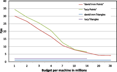

  

  Comparing triangles and points as rendering primitives on parallel multi-machine large displays

The same observation is reinforced from Fig. 8. This implies that one could obtain a close to one order of magnitude of speed-up when rendering points in comparison to triangles without losing too much on the quality front.

7 Conclusion and future work

We have presented an efficient framework for hierarchical multi-resolution pre-processing and rendering of massive point cloud datasets which can support high quality rendering using geo-morphing and smooth point interpolation. Our fast, high quality pre-processing methods improve upon the state-of-art to obtain targeted number of output points which can be efficiently kept as VBOs. We have demonstrated that our novel point hierarchy definition is flexible in that it can adapt to a desired LOD granularity by adjusting its fan-out factor N that we can target specific rendering-efficient VBO sizes, and that our algorithm supports adaptive out-of-core rendering, featuring asynchronous pre-fetching and loading from disk as well as rendering on a budget.

Related future work could include better compression schemes to reduce the per node VBO data size while still allowing it to be used by the GPU with minimal runtime processing overhead on the CPU, and to apply extensions that make the approach suitable for streaming over network and remote rendering.

References

Goswami, P., Zhang, Y., Pajarola, R., Gobbetti, E.: High quality interactive rendering of massive point models using multi-way kd-trees. In: Proceedings Pacific Graphics Poster Papers, pp. 93–100 (2010)
Levoy, M., Whitted, T.: The use of points as display primitives. TR 85-022, Technical Report, Department of Computer Science, University of North Carolina at Chapel Hill (1985)
Grossman, J.P., Dally, W.J.: Point sample rendering. In: Proceedings Eurographics Workshop on Rendering, pp. 181–192 (1998)
Pfister, H., Gross, M.: Point-based computer graphics. IEEE Comput. Graph. Appl. 24(4), 22–23 (2004)
Gross, M.H.: Getting to the point…? IEEE Comput. Graph. Appl. 26(5), 96–99 (2006)
Gross, M.H., Pfister, H.: Point-Based Graphics. Morgan Kaufmann, San Mateo (2007)
Sainz, M., Pajarola, R.: Point-based rendering techniques. Comput. Graph. 28(6), 869–879 (2004)
Kobbelt, L., Botsch, M.: A survey of point-based techniques in computer graphics. Comput. Graph. 28(6), 801–814 (2004)
Rusinkiewicz, S., Levoy, M.: QSplat: A multiresolution point rendering system for large meshes. In: Proceedings ACM SIGGRAPH, pp. 343–352 (2000)
Grottel, S., Reina, G., Dachsbacher, C., Ertl, T.: Coherent culling and shading for large molecular dynamics visualization. Comput. Graph. Forum 29(3), 953–962 (2010) (Proceedings of EUROVIS)
Dachsbacher, C., Vogelgsang, C., Stamminger, M.: Sequential point trees. ACM Trans. Graph. 22(3) (2003). Proceedings ACM SIGGRAPH
Pajarola, R., Sainz, M., Lario, R.: XSplat: External memory multiresolution point visualization. In: Proceedings IASTED International Conference on Visualization, Imaging and Image Processing, pp. 628–633 (2005)
Wimmer, M., Scheiblauer, C.: Instant points: Fast rendering of unprocessed point clouds. In: Proceedings Eurographics/IEEE VGTC Symposium on Point-Based Graphics, pp. 129–136 (2006)
Gobbetti, E., Marton, F.: Layered point clouds. In: Proceedings Eurographics/IEEE VGTC Symposium on Point-Based Graphics, pp. 113–120 (2004)
Wand, M., Berner, A., Bokeloh, M., Fleck, A., Hoffmann, M., Jenke, P., Maier, B., Staneker, D., Schilling, A.: Interactive editing of large point clouds. In: Proceedings Eurographics/IEEE VGTC Symposium on Point-Based Graphics, pp. 37–46 (2007)
Bettio, F., Gobbetti, E., Martio, F., Tinti, A., Merella, E., Combet, R.: A point-based system for local and remote exploration of dense 3D scanned models. In: Proceedings Eurographics Symposium on Virtual Reality, Archaeology and Cultural Heritage, pp. 25–32 (2009)
Pauly, M., Gross, M., Kobbelt, L.P.: Efficient simplification of point-sampled surfaces. In: Proceedings IEEE Visualization, pp. 163–170 (2002)
Bierbaum, A., Just, C., Hartling, P., Meinert, K., Baker, A., Cruz-Neira, C.: VR Juggler: A virtual platform for virtual reality application development. In: Proceedings IEEE Virtual Reality, pp. 89–96 (2001)
Humphreys, G., Houston, M., Ng, R., Frank, R., Ahern, S., Kirchner, P.D., Klosowski, J.T.: Chromium: A stream-processing framework for interactive rendering on clusters. ACM Trans. Graph. 21(3) (2002). Proceedings ACM SIGGRAPH
Eilemann, S., Makhinya, M., Pajarola, R.: Equalizer: A scalable parallel rendering framework. IEEE Trans. Vis. Comput. Graph. 15(3), 436–452 (2009)
Goswami, P., Makhinya, M., Bösch, J., Pajarola, R.: Scalable parallel out-of-core terrain rendering. In: Eurographics Symposium on Parallel Graphics and Visualization, pp. 63–71 (2010)
Corea, W.T., Klosowski, J.T., Silva, C.T.: Out-of-core sort-first parallel rendering for cluster-based tiled displays. In: Fourth Eurographics Workshop on Parallel Graphics and Visualization, pp. 63–71 (2002)
Hubo, E., Bekaert, P.: A data distribution strategy for parallel point-based rendering. In: Proceedings International Conference on Computer Graphics, Visualization and Computer Vision, pp. 1–8 (2005)
Zhang, Y., Pajarola, R.: Deferred blending: Image composition for single-pass point rendering. Comput. Graph. 31(2), 175–189 (2007)
Corrêa, W.T., Fleishman, S., Silva, C.T.: Towards point-based acquisition and rendering of large real-world environments. In: Proceedings of the 15th Brazilian Symposium on Computer Graphics and Image Processing, p. 59 (2002)
Molnar, S., Cox, M., Ellsworth, D., Fuchs, H.: A sorting classification of parallel rendering. IEEE Comput. Graph. Appl. 14(4), 23–32 (1994)
MacQueen, J.B.: Some methods for classification and analysis of multivariate observations. In: Proceedings of 5th Berkeley Symposium on Mathematical Statistics and Probability, pp. 281–297. University of California Press, Berkeley (1967)
Dasgupta, S.: The hardness of k-means clustering. CS2008-0916, Technical Report, Department of Computer Science and Engineering University of California, San Diego (2008)
Acknowledgements
We would like to thank and acknowledge the Stanford 3D Scanning Repository and Digital Michelangelo projects as well as Roberto Scopigno, for the Pisa Cathedral model, for providing the 3D geometric test datasets used in this paper. This work was supported in parts by the Swiss Commission for Technology and Innovation (KTI/CTI) under Grant 9394.2 PFES-ES.
Author information
Authors and Affiliations
Corresponding author
Electronic Supplementary Material
Below is the link to the electronic supplementary material.
Rights and permissions
About this article
Cite this article
Goswami, P., Erol, F., Mukhi, R. et al. An efficient multi-resolution framework for high quality interactive rendering of massive point clouds using multi-way kd-trees. Vis Comput 29, 69–83 (2013). https://doi.org/10.1007/s00371-012-0675-2
Published:
Issue Date:
DOI: https://doi.org/10.1007/s00371-012-0675-2